First principles calculation of conductance and current flow through low-dimensional superconductors

Abstract

We present a novel formulation to calculate transport through disordered superconductors connected between two metallic leads. An exact expression for the current is derived, and is applied to a superconducting sample described by the negative-$U$ Hubbard model. A Monte Carlo algorithm that includes thermal phase and amplitude fluctuations of the superconducting order parameter is employed, and a new efficient algorithm is described. This improved routine allows access to relatively large systems, which we demonstrate by applying it to several cases, including superconductor-normal interfaces and Josephson junctions. The effects of decoherence and dephasing are shown to be included in the formulation, which allows the unambiguous characterization of the Kosterlitz-Thouless transition in two-dimensional systems and the calculation of the finite resistance due to vortex excitations in quasi one-dimensional systems. Effects of magnetic fields can be easily included in the formalism, and are demonstrated for the Little-Parks effect in superconducting cylinders. Moreover, the formalism enables us to map the local super and normal currents, and the accompanying electrical potentials, which we use to pinpoint and visualize the emergence of resistance across the superconductor-insulator transition.

I Introduction

Chief amongst the remarkable effects observed in superconductors is their eponymous perfect conductivity. Within BCS theory BCS , where superconductivity arises due to pairing between electrons, the effects of temperature $T$, magnetic field $B$, and disorder are well understood: as the pairing amplitude is suppressed by these physical parameters, the system becomes normal, and attains a finite resistance. For low-dimensional systems, on the other hand, it has been long understood that phase fluctuations of the pairing amplitude play a major role in the loss of perfect conductance Halperin . In two-dimensional systems, for example, it has been demonstrated BKT that as the temperature increases there is a critical temperature $T_{\text{KT}}$ where vortices and anti-vortices unbind and proliferate through the system, leading to the loss of global phase coherence and superconductivity, even though the pairing amplitude remain finite. Indications of such a Berezinsky-Kosterlitz-Thouless (BKT) transition have been observed in Josephson-junction arrays KTarray , in superconducting (SC) thin films Yazdani93 , and possibly in high-$T_{\text{c}}$ cuprates KTinHighTc .

In recent years there has been a reinvigoration of research into low-dimensional superconductors. This has been motivated by intriguing experimental observations of electronic transport through disordered SC thin films, such as a huge magnetoresistance peak MR and a “super-insulator” phase SI , and by the technological progress in producing two-dimensional superconductors in the interface between two oxides LaSr and in making ultra-thin cuprate superconductors UltraThin . Many of these observations are not yet satisfactory explained, chiefly because there is no theory that can calculate the current, even numerically, through a disordered superconductor, based on a microscopic model.

The calculation of the resistance within the BCS picture, usually based on the Bogoliubov-de Gennes (BdG) mean-field approach, is straightforward. Blonder, Tinkham, and Klapwijk (BTK) Blonder82 studied the reflectance and transmission at a metal-superconductor junction, and an analogous study was performed at superconductor-metal-superconductor junctions Kulik70 . Similar approaches resistance utilized the Buttiker-Landauer picture Landauer57 ; Buttiker86 for non-interacting Cooper pairs to study scattering through a SC region. (A difficulty with the direct application of the BdG formalism is the non-conservation of charge, which can be overcome by studying a normal ring containing a SC segment EntinWohlman08 .) An alternative approach near to the BCS critical temperature is to use a scaling assumption for the conductivity Dorsey91 . The current through diffusive normal metal-superconductor structures has also been calculated using a Keldysh scattering matrix theory Stoof95 . All these approaches neglect phase fluctuations so cannot be used to study two-dimensional superconductors that exhibit a BKT-like transition at low temperatures.

The resistance of low-dimensional superconductors can also be calculated using phenomenological models. The conductivity of uniform systems can be probed analytically by studying phase slips across the sample within the Ginzburg-Landau approach Langer67 ; McCumber70 . Thermally excited phase slips explain both non-linear conductivity and vortex creep induced resistance Halperin79 , whilst quantum activated phase slips can drive SC wires insulating Buchler04 . However, phenomenological calculations are neither underpinned by a microscopic model nor include Coulomb repulsion or disorder except for the introduction of a phenomenological normal state resistance.

Here we develop a new formalism to calculate the current through a superconductor taking into account phase fluctuations in the presence of disorder, finite $T$ and $B$, and Coulomb repulsion. The approach we detail here is based on the Landauer-Buttiker scheme Landauer57 ; Buttiker86 , where one attaches metallic leads to the sample, and then calculate its conductance. The lead-superconductor tunneling barriers ensure that the conductance of the system is always finite, even in the SC phase. A previous attempt using the quantum Monte Carlo approach to calculate current in disordered systems employed the fluctuation-dissipation theorem via the current-current correlation function Trivedi96 .

The Landauer formula Landauer57 ; Buttiker86 is a widely adopted method to calculate the current through a mesoscopic sample that contains non-interacting particles. Meir and Wingreen Meir92 have generalized the formula to produce an exact expression for the current through any interacting region attached to non-interacting leads, which has been successfully applied to a wide range of systems. Following this approach, we partition the system into the three parts shown in Fig. 1: the left-hand lead, the central interacting region, here a superconductor, and the right-hand lead. In the leads the natural particle basis set are electrons, and in the sample the natural basis set are Bogoliubons. To circumvent this mismatch of particle basis sets we reformulate the Meir-Wingreen formula in a Bogoliubon basis set to derive an exact expression for the current flow through a possibly SC region, attached to two metallic leads.

Figure 1: (Color online) A schematic of the experimental setup within the negative-$U$ Hubbard model. The left and right-hand metallic leads are shown in blue, from which electrons can tunnel through the barriers shown by the gray links into the central SC region which is shown in red.

Having derived a general, exact formula, the SC region is then modeled by a generalized negative-$U$ Hubbard model based on the lattice shown in Fig. 1. Introducing two local auxiliary fields (which reduce to the local density and gap at zero temperature), we decouple the interacting fermions. While the conductance formula is exact, in order to evaluate correlation functions we neglect quantum fluctuations, and integrate numerically over the thermal fluctuations of the auxiliary parameters Mayr ; Erez2010 using a Monte Carlo method. A significant advantage of the formalism is that it allows us to construct current and potential maps of the system. These allow us to diagnose the microscopic features that increase the resistance of the sample. This paper details the new procedure and presents a number of applications of the formalism for simple systems, where one can compare with existing theories.

The paper is organized as follows: in Sec. II we first derive an exact expression for the current through a SC region. Using this expression, in Sec. III we describe how the current can be calculated numerically and outline improvements to the auxiliary field approach that allows us to study large systems. Having developed the new formula for the current and accompanying computational tool, it is vital to carefully test it against a series of known results. Therefore, in Sec. IV.1 we study superconductor-normal interfaces in clean systems, and compare with the BTK transmission formulae, while in Sec. IV.2 we study the temperature dependent current in a Josephson junction. In Sec. IV.3 we describe how effects of decoherence and dephasing are manifested in the formalism. We investigate the temperature dependence of resistance in Sec. IV.4 in which we uncover the temperature dependence of the resistance and the nonlinear $I-V$ behavior that characterizes the BKT transition in two dimensions and vortex excitations in quasi one-dimensional systems. We then, in Sec. IV.5, apply an external magnetic field to probe the Little-Parks effect. Finally, we demonstrate how to construct current and potential maps for the system, and use them to study the microscopic behavior at the superconductor-insulator transition in Sec. IV.6. The details of the analytical derivation and the numerical procedure are described in the appendices.

II Analytical Derivation

II.1 Current Formula

To calculate the current for interacting particles we start with the general formula for the current Meir92 through an interacting region, connected between two non-interacting leads

$$J=\frac{\text{i}e}{2h}\sum_{\sigma}\int\text{d}\epsilon\Bigl{[} \operatorname{Tr}\left\{\left(f_{\text{L}}(\epsilon)\mathsf{\Gamma}^{\text{L}}-f_{\text{R}}(\epsilon)\mathsf{\Gamma}^{\text{R}}\right)\left({\cal G}_{\sigma}^{\text{r}}-{\cal G}_{\sigma}^{\text{a}}\right)\right\}$$

$$+ \operatorname{Tr}\left\{(\mathsf{\Gamma}^{\text{L}}-\mathsf{\Gamma}^{\text{R}}){\cal G}_{\sigma}^{<}\right\}\Bigr{]}\,.$$ (1)

Here $f_{\chi}(\epsilon)\equiv[\exp(\beta(\epsilon-\mu_{\chi}))+1]^{-1}$ with $\chi\in\{\text{L},\text{R}\}$ is the Fermi distribution of the left (L) and right-hand (R) leads that are held at chemical potentials $\mu_{\chi}$ and reduced temperature $\beta\equiv 1/k_{\text{B}}T$ (where $k_{B}$ is the Boltzmann constant). The imposed potential difference $eV\equiv\Delta\mu=\mu_{\text{L}}-\mu_{\text{R}}$ between the leads drives the current $J$ through the system. The integral is over all electronic energies $\epsilon$. $\mathsf{\Gamma}^{\chi}_{ij}\equiv 2\pi\sum_{a\in\chi}\rho_{a}(\epsilon)Y_{ai}Y_{aj}^{*}$ for channels $a$ in lead $\chi$, and $Y_{a,i}$ is the tunneling matrix element from channel $a$ in the the lead to site $i$ in the sample. Finally, ${\cal G}_{ij\sigma}^{\text{r}}$, ${\cal G}_{ij\sigma}^{\text{a}}$, and ${\cal G}_{ij\sigma}^{<}$ are the electronic retarded, advanced, and lesser Green functions (in the site basis) for electrons of spin $\sigma$ in the sample calculated in the presence of the leads.

Eqn. (1) is exact, and captures, via the electronic Green function ${\cal G}$, all the processes that can transfer an electron through the system. When the intermediate regime has SC correlations, some of these processes involve Andreev scattering – absorption of an electron pair by the condensate and a propagation of the remaining hole. To expose these processes, it is convenient to transform from the electron basis set $(c_{i\sigma}^{\dagger},c_{i\sigma})$ with site index $i$ into the Bogoliubov basis set $(\gamma_{n\sigma}^{\dagger},\gamma_{n\sigma})$, using the Bogoliubov-de Gennes relations $c_{i\sigma}=\sum_{n}u_{i}(n)\gamma_{n\sigma}-\sigma v_{i}^{*}(n)\gamma_{n-\sigma}^{\dagger}$ (at present $u_{i}$ and $v_{i}$ are arbitrary, except for the unitarity condition, but later on they will be determined by the actual Hamiltonian that will be used for the SC region). The Green functions transform from the electron basis ${\cal G}_{\sigma}$ into the energy basis set of Green functions $\{\mathsf{G}_{\sigma}^{>},\mathsf{G}_{\sigma}^{<}\}$ and the family of anomalous Green functions $\mathsf{H}^{>}_{\sigma}(m,n)=-\text{i}\langle\gamma_{m-\sigma}^{\dagger}\gamma_{n\sigma}^{\dagger}\rangle$, $\mathsf{H}^{<}_{\sigma}(m,n)=\text{i}\langle\gamma_{n-\sigma}^{\dagger}\gamma_{m\sigma}^{\dagger}\rangle$, $\bar{\mathsf{H}}^{>}_{\sigma}(m,n)=-\text{i}\langle\gamma_{m-\sigma}\gamma_{n\sigma}\rangle$, and $\bar{\mathsf{H}}^{<}_{\sigma}(m,n)=\text{i}\langle\gamma_{n-\sigma}\gamma_{m\sigma}\rangle$ according to

$${\cal G}_{\sigma}^{\text{r}}(i,j)-{\cal G}_{\sigma}^{\text{a}}(i,j)={\cal G}_{\sigma}^{>}(i,j)-{\cal G}_{\sigma}^{<}(i,j)$$

$$=\mathbf{u}_{i}\left(\mathsf{G}_{\sigma}^{>}-\mathsf{G}_{\sigma}^{<}\right)\mathbf{u}_{j}^{*}+\mathbf{v}_{i}\left(\mathsf{G}_{-\sigma}^{>}-\mathsf{G}_{-\sigma}^{<}\right)\mathbf{v}_{j}^{*}$$

$$-\sigma\mathbf{v}_{i}^{*}\left(\mathsf{H}_{\sigma}^{>}-\mathsf{H}_{\sigma}^{<}\right)\mathbf{u}_{j}^{*}-\sigma\mathbf{u}_{i}\left(\bar{\mathsf{H}}_{-\sigma}^{>}-\bar{\mathsf{H}}_{-\sigma}^{<}\right)\mathbf{v_{j}}\,,$$ (2)

and

$${\cal G}_{\sigma}^{<}(i,j)\!=\!\mathbf{u}_{j}^{*}\mathsf{G}^{<}_{\sigma}\mathbf{u}_{i}^{*}\!-\!\mathbf{v}_{j}\mathsf{G}^{>}_{-\sigma}\mathbf{v}_{i}^{*}\!+\!\sigma\mathbf{u}^{*}_{j}\mathsf{H}_{\sigma}^{>}\mathbf{v}^{*}_{i}\!-\!\sigma\mathbf{v}_{j}\bar{\mathsf{H}}_{-\sigma}^{<}\mathbf{u}_{i}\!\,.$$ (3)

Solving for the Green functions across the system in the presence of the leads (Appendix A), leads to the final, exact result

$$J=\frac{e}{h}\sum_{\sigma}\int\text{d}\epsilon[f_{\text{L}}(\epsilon)-f_{\text{R}}(\epsilon)]\times$$

$$\operatorname{Tr}\Bigl{[} (\mathsf{\Gamma}_{\mathsf{u}^{*}\mathsf{u}}^{\chi}+\mathsf{\Gamma}_{\mathsf{v}^{*}\mathsf{v}}^{\chi})\mathsf{G}_{\sigma}^{\text{a}}(\mathsf{\Gamma}_{\mathsf{u}\mathsf{u}^{*}}^{-\chi}-\mathsf{\Gamma}_{\mathsf{v}\mathsf{v}^{*}}^{-\chi})\mathsf{G}_{\sigma}^{\text{r}}$$

$$+ (\mathsf{\Gamma}_{\mathsf{u}\mathsf{v}}^{\chi}-\mathsf{\Gamma}_{\mathsf{v}\mathsf{u}}^{\chi})\mathsf{G}_{\sigma}^{\text{a}}\mathsf{\Gamma}_{\mathsf{v}^{*}\mathsf{u}^{*}}^{-\chi}\mathsf{H}_{\sigma}^{\text{r}}+(\mathsf{\Gamma}_{\mathsf{u}^{*}\mathsf{v}^{*}}^{\chi}-\mathsf{\Gamma}_{\mathsf{v}^{*}\mathsf{u}^{*}}^{\chi})\mathsf{G}_{\sigma}^{\dagger\text{a}}\mathsf{\Gamma}_{\mathsf{u}\mathsf{v}}^{-\chi}\mathsf{H}_{\sigma}^{\dagger\text{r}}$$

$$+ \sigma\mathsf{\Gamma}_{\mathsf{u}\mathsf{u}^{*}}^{\chi}\mathsf{H}_{\sigma}^{\text{a}}(\mathsf{\Gamma}_{\mathsf{v}^{*}\mathsf{u}^{*}}^{-\chi}\!\!-\!\mathsf{\Gamma}_{\mathsf{u}^{*}\mathsf{v}^{*}}^{-\chi})\mathsf{G}_{\sigma}^{\text{r}}\!+\!\sigma\mathsf{\Gamma}_{\mathsf{v}\mathsf{v}^{*}}^{\chi}\mathsf{H}_{\sigma}^{\dagger\text{a}}(\mathsf{\Gamma}_{\mathsf{v}\mathsf{u}}^{-\chi}\!\!-\!\mathsf{\Gamma}_{\mathsf{u}\mathsf{v}}^{-\chi})\mathsf{G}_{\sigma}^{\dagger\text{r}}$$

$$+ \sigma(\mathsf{\Gamma}_{\mathsf{u}\mathsf{u}^{*}}^{\chi}+\mathsf{\Gamma}_{\mathsf{v}\mathsf{v}^{*}}^{\chi})(\mathsf{H}_{\sigma}^{\text{a}}\mathsf{\Gamma}_{\mathsf{v}^{*}\mathsf{u}^{*}}^{-\chi}\mathsf{H}_{\sigma}^{\text{r}}+\mathsf{H}_{\sigma}^{\dagger\text{a}}\mathsf{\Gamma}_{\mathsf{u}\mathsf{v}}^{-\chi}\mathsf{H}_{\sigma}^{\dagger\text{r}})\Bigr{]}\,,$$ (4)

where $\mathsf{\Gamma}^{\chi}_{\mathsf{u}\mathsf{v}}(m,n)=2\pi\sum_{i,j,a\in\chi}\rho_{a}(\epsilon)Y_{ai}Y_{aj}\mathsf{u}_{i}(m)\mathsf{v}_{j}(n)$ is now in the transformed basis set. This is written in a form describing transmission from the left-hand side to the right-hand side of the sample. We will show in Sec. IV.1 that it therefore exposes the rise of resistance due to the suppression of correlations between the left and right-hand sides of the superconductor.

We note that deep in the SC regime where the SC gap obeys $\Delta\gg Y$, and in the case where the leads inject electrons within the gap such that $eV<2\Delta$, we can make a perturbative expansion in small tunneling $Y$. This yields the simple expression for the current

$$J= \frac{e}{h}\sum_{\sigma}\int\text{d}\epsilon[f_{\text{L}}(\epsilon)-f_{\text{R}}(\epsilon)]\times$$

$$\operatorname{Tr}\left[(\mathsf{\Gamma}_{\mathsf{u}^{*}\mathsf{u}}^{\chi}+\mathsf{\Gamma}_{\mathsf{v}^{*}\mathsf{v}}^{\chi})\tilde{\mathsf{G}}_{\sigma}^{\text{a}}(\mathsf{\Gamma}_{\mathsf{u}\mathsf{u}^{*}}^{-\chi}-\mathsf{\Gamma}_{\mathsf{v}\mathsf{v}^{*}}^{-\chi})\tilde{\mathsf{G}}_{\sigma}^{\text{r}}\right]\,.$$ (5)

Here $\tilde{\mathsf{G}}$ are the Green functions calculated in the absence of the leads. This equation has direct $Y^{4}$ dependence on the tunneling matrix element, with neglected higher order contributions of order $\sim(Y/\Delta)^{6}$, as it describes Cooper pairs tunneling through the contact barrier. We shall show later that this contribution is precisely what is predicted for the current Lambert91 according to the BTK formula Blonder82 , and notably, as the leads inject electrons only into the gap, there is no normal current, but only Andreev processes allow the flow of current. The perturbative form Eqn. (5) offers two important computational advantages. Firstly, it is considerably less resource intensive to calculate as the Green functions are diagonal so it does not demand summations over separate variables. Secondly, it does not require the expensive matrix inversion embodied in Eqn. (28) to find the general equation for the current. Due to its usefulness we also note that an analogous expression can be derived for the normal current when injecting electrons outside of the gap

$$J=\frac{e}{h}\sum_{\sigma}\int\text{d}\epsilon\operatorname{Tr}[ f_{\text{L}}(\epsilon)(\mathsf{\Gamma}_{\mathsf{u}^{*}\mathsf{u}}^{\chi}+\mathsf{\Gamma}_{\mathsf{v}^{*}\mathsf{v}}^{\chi})$$

$$- f_{\text{R}}(\epsilon)(\mathsf{\Gamma}_{\mathsf{u}^{*}\mathsf{u}}^{\chi}+\mathsf{\Gamma}_{\mathsf{v}^{*}\mathsf{v}}^{\chi})]\Im\mathsf{G}_{\sigma}^{\text{r}}\,,$$ (6)

where $\Im$ stands for the imaginary part. Since this term represents the normal current, it has a direct $Y^{2}$ dependence on the tunneling matrix element. Though they offer a considerable computational advantage, these perturbative formulae cannot be used on the border of the superconductor-insulator transition where the superconductor gap breaks down and $\Delta<Y$. Therefore, unless specified, we use the full expression for the current, Eqn. (4), in our numerical calculations.

II.2 Current and voltage maps

Eqn. (6), with a coefficient of $Y^{2}$, describes the normal current that enters and leaves the system as single electrons, whereas Eqn. (5) with a coefficient of $Y^{4}$ corresponds to a tunneling supercurrent. However, the normal and supercurrent can interchange inside the sample. In order to understand the microscopics behind phenomena in the disordered superconductor it is vital that we can probe the spatial distribution of the current as it switches in nature through the sample. Therefore, here we extend our formalism to map out the flow of current within the sample. To calculate the current distribution map we use the general expression for the current crossing a single bond Caroli71 ; Cresti03 from site $i$ to $j$

$$J_{ij}=\frac{2e}{h}\sum_{\sigma}\int\frac{\text{d}\epsilon}{2\pi}\left[t_{ij}{\cal G}_{\sigma}^{<}(j,i)-t_{ji}{\cal G}_{\sigma}^{<}(i,j)\right]\,.$$ (7)

Transforming again into the diagonalized basis, the local current is

$$J_{ij}= \frac{2e}{h}\sum_{\sigma}\!\int\!\frac{\text{d}\epsilon}{2\pi}\operatorname{Tr}\biggl{\{}\!\left[\mathsf{\Lambda}^{ij}_{\mathsf{u}^{*}\mathsf{u}}\!-\!\mathsf{\Lambda}^{ij}_{\mathsf{v}^{*}\mathsf{v}}\right]\!\mathsf{G}_{\sigma}^{<}\!-\!\left[\mathsf{\Lambda}^{ij\text{T}}_{\mathsf{u}\mathsf{u}^{*}}\!-\!\mathsf{\Lambda}^{ij\text{T}}_{\mathsf{v}\mathsf{v}^{*}}\right]\!\mathsf{G}_{\sigma}^{<}$$

$$+ \sigma\left[\mathsf{\Lambda}^{ij\text{T}}_{\mathsf{v}^{*}\mathsf{u}^{*}}-\mathsf{\Lambda}^{ij}_{\mathsf{u}^{*}\mathsf{v}^{*}}\right]\mathsf{H}_{\sigma}^{<}+\sigma\left[\mathsf{\Lambda}^{ij\text{T}}_{\mathsf{u}\mathsf{v}}-\mathsf{\Lambda}^{ij}_{\mathsf{v}\mathsf{u}}\right]\bar{\mathsf{H}}_{\sigma}^{<}\biggr{\}}\,,$$ (8)

where $\mathsf{\Lambda}^{ij}_{\mathbf{u}\mathbf{v}}(m,n)=t_{ij}\mathbf{u}_{i}(m)\mathbf{v}_{j}(n)$. As before, the normal $\mathsf{G}^{<}$ and anomalous Green functions $\mathsf{H}^{<}$ are calculated in Eqn. (35) in the presence of the leads. Moreover we note that the current comes in two flavors, the contribution to the current from the normal Green function $\mathsf{G}^{<}$ is associated with the normal current and that from the anomalous Green function $\mathsf{H}^{<}$ gives the Cooper pair current. In Sec. IV.6 we verify that this intersite current yields the correct net conservation of charge.

To provide an additional probe into the nature of the superconductor-insulator transition we extend the formalism to map the local chemical potentials across the sample. This should reveal any weak links and the location of the sources of resistance in a sample. To determine the local effective potential at a specific site we add a weak link from that site to a third lead (a “tip”). The tunneling current from the tip into the sample is then calculated, and the chemical potential of the tip adjusted until that current flow is zero. This chemical potential thus corresponds to the effective local chemical potential in that site. To calculate the current flow into the tip we first evaluate the full Green functions $\mathsf{G}$ in the sample in the presence of voltage drop between the left and right reservoirs Eqn. (28) but without the tip. We then use the perturbative formula for the current, Eqn. (5), but with one lead representing the left/right hand leads, and the other the perturbative tip. This process is repeated for each site in the sample (due to the perturbative nature of the tip, this calculation can be done simultaneously for all sites). In Sec. IV.6 we demonstrate how maps of the potential can expose weak links in the sample and help diagnose the microscopic mechanisms that give rise to resistance.

III Model and Numerical procedure

In the previous section we have developed an exact formula for the current through an arbitrary intermediate region, which may include SC correlations. We now use a specific model to describe this SC region – the negative-$U$ Hubbard model, a lattice model that includes on-site attraction, and may include disorder, orbital and Zeeman magnetic fields, and even long-range repulsive interaction (which we will not deal with in this paper). The Hamiltonian is

$$\hat{H}_{\text{Hubbard}} \!=\!\sum_{i,\sigma}\epsilon_{i\sigma}c^{\dagger}_{i\sigma}c_{i\sigma}\!-\sum_{i}U_{i}c^{\dagger}_{i\uparrow}c^{\dagger}_{i\downarrow}c_{i\downarrow}c_{i\uparrow}$$

$$-\!\!\!\sum_{\langle i,j\rangle,\sigma}\!\left(t_{ij}c^{\dagger}_{i\sigma}c_{j\sigma}+t_{ij}^{*}c^{\dagger}_{j\sigma}c_{i\sigma}\right)\,,$$ (9)

where $\epsilon_{i\sigma}$ is the on-site energy, $t_{ij}$ the hopping element between adjacent sites $i$ and $j$, and $U_{i}$ is the onsite two-particle attraction, taken to be uniform, $i$-independent, in this paper. An orbital magnetic field can be incorporated into the phases of the hopping elements $t_{ij}$, while a Zeeman field splits the spin-dependent on-site energies $\epsilon_{i\sigma}$. In this paper we will only deal with orbital fields. To account for disorder, $\epsilon_{i}$ will be drawn from a Gaussian distribution with characteristic width $W$. The inter-site spacing is $a$. Unlike, for example, the disordered XY model, the negative-$U$ Hubbard model can lead to a BCS transition, a BKT transition, or to a percolation transition, and thus this choice is general enough not to limit a priori the underlying physical processes. Importantly, the model includes the fermionic degrees of freedom which may be relevant to some of the experimental observations.

Calculation of correlation functions, for example the Green functions that enter the current formula, require thermal averages. To perform the thermal average we need to decouple the quartic interaction term so we employ the exact Hubbard-Stratonovich transformation

$$\text{e}^{-\int_{0}^{\beta}\text{d}\tau\sum_{i}U_{i}c_{i\uparrow}^{\dagger}c_{i\downarrow}^{\dagger}c_{i\downarrow}c_{i\uparrow}}=$$

$$\int\mathcal{D}\Delta\mathcal{D}\bar{\Delta}\text{e}^{-\int_{0}^{\beta}\text{d}\tau\sum_{i}{\frac{-\left|\Delta_{i}(\tau)\right|^{2}}{U_{i}}+\Delta_{i}(\tau)c_{i\uparrow}^{\dagger}c_{i\downarrow}^{\dagger}+\bar{\Delta}_{i}(\tau)c_{i\downarrow}c_{i\uparrow}}},$$ (10)

which is basically a Gaussian integration ($\mathcal{D}\Delta\equiv\Pi_{\tau,i}\text{d}\Delta_{i}(\tau)$, where the product runs over all times and all sites). Note that the field $\Delta_{i}(\tau)$ is just an integration variable that decouples the two-body term in the superconducting channel, and should not be confused with $|U_{i}|\langle c_{i\downarrow}c_{i\uparrow}\rangle$. Similarly, one introduces the integration fields $\rho_{i\sigma}(\tau)$, that couple to the spin density Altland06 $\langle c_{i\sigma}^{\dagger}c_{i\sigma}\rangle$, and leads to an additional term $-\sum_{i,\sigma}|U_{i}|\rho_{i-\sigma}(\tau)c_{i\sigma}^{\dagger}c_{i\sigma}$ in the action (which, in the mean-field approximation gives rise to the Hartree-Fock contribution) . Decoupling in both the $\Delta$ and $\rho$ channels not only provides access to both soft degrees of freedom, but also the saddle point solution gives the standard mean-field results for those fields, and furthermore guarantees that the action expanded to Gaussian order corresponds to the random phase approximation DePalo99 .

The Hubbard-Stratonovich transformation (10) is exact. Since our main interest lies in thermal effects, for example the thermal BKT phase transition, or thermal activation of vortices, we now neglect quantum fluctuations (the $\tau$ dependence of $\Delta$). One can now write the partition function for the Hubbard model as Mayr ; Erez2010

$$\mathcal{Z}=\operatorname{Tr}\left[\text{e}^{-\beta\hat{H}_{\text{Hubbard}}}\right]=\int\mathcal{D}(\bm{\Delta},\bm{\rho})\operatorname{Tr}_{\text{f}}\left[\text{e}^{-\beta\mathcal{\hat{H}}_{\text{BdG}}(\bm{\Delta},\bm{\rho})}\right]$$ (11)

where the latter trace is over all fermionic degrees of freedom. $\mathcal{H}_{\text{BdG}}(\bm{\Delta},\bm{\rho})$ is the Bogoliubov-de Gennes (BdG) Hamiltonian with a given set of $\bm{\Delta}$ and $\bm{\rho}$, where these vectors designate the set of values of these parameters on all lattice sites

$$\hat{\mathcal{H}}_{\text{BdG}}=\sum_{i,\sigma}(\epsilon_{i}+\rho_{i})c^{\dagger}_{i\sigma}c_{i\sigma}-\!\!\sum_{\langle i,j\rangle,\sigma}\!\left(t_{ij}c^{\dagger}_{i\sigma}c_{j\sigma}+t_{ij}^{*}c^{\dagger}_{j\sigma}c_{i\sigma}\right)$$

$$+\sum_{i}\left(\Delta_{i}c^{\dagger}_{i\uparrow}c^{\dagger}_{i\downarrow}+\bar{\Delta}_{i}c_{i\downarrow}c_{i\uparrow}\right)+\sum_{i}\frac{|\Delta_{i}|^{2}+\rho_{i}^{2}}{U_{i}}\,.$$ (12)

Given the explicit form of the diagonalizable BdG Hamiltonian, we can calculate expectation values and correlation functions,

$$\operatorname{Tr}\left[\hat{\rho}\ \!\hat{\mathcal{O}}\right]=\int\mathcal{D}(\bm{\Delta},\bm{\rho})\text{e}^{-\beta E_{0}}\sum_{n=1}^{N}\text{e}^{-\beta E_{n}}\left\langle n\left|\hat{\mathcal{O}}\right|n\right\rangle,$$ (13)

where the sum is taken over all positive eigenvalues (quasi-particle excitations) of the BdG Hamiltonian. Here $E_{0}$, $E_{n}$ and $|n\rangle$ are the ground-state energy, excitation energies and excitation wave functions, respectively, for the BdG Hamiltonian, for the specific configuration of $\bm{\Delta}$ and $\bm{\rho}$. It is straightforward to see that in this case, the saddle-point approximation of the partition function gives rise to the mean-field BdG equations (and then $\Delta_{i}$ indeed corresponds to $|U_{i}|\langle c_{i\downarrow}c_{i\uparrow}\rangle$). The calculation of the full integral, using the (classical) Monte Carlo approach Metropolis53 , includes also the contributions of thermal fluctuations of the amplitude and phase of the order parameter. In Appendix B we detail how we improve on contemporary methods to perform the Monte Carlo calculation in $\mathcal{O}(N^{1.9}M^{2/3})$ time, where $N$ is the number of sites and $M$ the order of a Chebyshev expansion.

IV Applications

We have derived a new expression for the current flow through a superconductor, and demonstrated how to calculate the current in mesoscopic systems. Before applying it to understand and predict novel phenomena, it is important to verify it across a variety of exemplar systems, where one can compare against well-established theories. As the main novelty of the approach is the inclusion of thermal fluctuations, we pay particular attention to verifying the formalism in two dimensions, especially looking for signatures of the BKT transition driven by phase fluctuations. In Sec. IV.1 we probe the current through a clean superconductor, and check that we can recover the BTK results for the contact resistance. A key effect in such systems is Josephson tunneling, so in Sec. IV.2 we study the temperature dependence of the resistance of a single Josephson junction. Dephasing (by temperature averaging) and decoherence (by electron-electron interactions) are studied in Sec. IV.3. In Sec. IV.4 we examine the temperature dependence of the resistance on the two sides of the BKT transition and compare to analytical results. In Sec. IV.5 we introduce finite magnetic field (flux) and probe the Little-Parks effect in the presence of disorder. Finally, in Sec. IV.6 we demonstrate how plotting maps of the current and potential across the system can illuminate the microscopic processes at the superconductor-insulator transition. Throughout we use an attractive interaction of $U=1.6t$ to describe the SC region. To avoid the Van Hove singularity at half filling Scalettar89 we study systems at an average $38.7\%$ filling, except for Sec. IV.3 where we focus on wires with a low filling fraction of $20\%$. In the linear response regime we impose a potential difference of $eV=0.02t$. Systems were typically two-dimensional, so a single lattice site thick, 12 lattice sites wide, and 48 lattice sites long.

IV.1 Clean systems

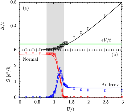
Figure 2: (Color online) The lower graph (b) shows the variation of conductance $\sigma$ with interaction strength. The normal current is shown in red and the supercurrent in blue. The numerical results are shown with error bars, and BTK theory by the solid line. The upper plot (a) shows the variation in the order parameter with interaction strength; numerics are shown with error bars and the mean-field theoretical prediction by the solid black line. The horizontal green line denotes the chemical potential difference across the sample. The gray shading denotes the range of interactions where $0<\Delta<eV$, so that both normal and Andreev processes contribute to the current.

At low temperatures, thermal fluctuations of the pair amplitude and phase may be neglected. The conductance, in this limit, through a clean SC region has been calculated by Blonder, Tinkham and Klapwijk (BTK) Blonder82 , and is solely due to the contact resistance at the two interfaces. By assigning a tunneling strength $1/Z$ to the barriers, BTK have shown that if the intermediate sample is in the normal state, then the current is purely due to electrons tunneling across the barrier, and the transmission coefficient is given by $1/Z^{2}$ Blonder82 . On the other hand, if the sample is in the SC state, then the SC gap, $\Delta$, inhibits electrons from directly tunneling into it. Instead, these electrons Andreev tunnel accompanied by a hole. For a large barrier $Z\gg 1$ the transmission coefficient becomes $\Delta^{2}/4Z^{4}(\Delta^{2}-E^{2})$ Blonder82 , where $E$ is the electron energy. Electrons with an energy outside of the gap can either tunnel alone with a corresponding normal transmission coefficient $(E+\sqrt{E^{2}-\Delta^{2}})/(2Z^{2}\sqrt{E^{2}-\Delta^{2}})$, or Andreev tunnel with accompanying hole, and have a transmission coefficient of $\Delta^{2}/4Z^{4}(E^{2}-\Delta^{2})$. We first compare the results of our numerical calculations to these BTK formulae, and then demonstrate that for the simple case of a single SC site, the BTK results can be derived analytically from our current formula.

To verify that the model recovers the correct behavior at the tunneling barrier we focus on the weak coupling limit. In this limit, once a Cooper pair tunnels through the first barrier, it has an equal probability of continuing to either the left or the right lead, an consequently the current through the double barrier will be half that of a single barrier Lambert91 . For a long enough system the finite bias and temperature smear any Fabry-Perot type interference. To study the effect of the changing order parameter $\Delta$, we focus on a $39\%$ filled system at “zero” temperature (without quantum fluctuations), where $\Delta$ is indeed equal to the pair correlation $|U|\langle c_{i\downarrow}c_{i\uparrow}\rangle$, vary the interaction strength $U$, and monitor the various components of the tunneling current. For a pristine system with $W=0$, all of the resistance stems from the two tunneling barriers, and we verified that the current flow was independent of the length of the SC region. A relatively large potential bias of $eV=0.1t$ was applied across the leads. This allows us to explore all tunneling processes, either for $\Delta<eV$ or $\Delta>eV$ by changing the interaction parameter $U$ and as a result $\Delta$, see Fig. 2(a). Our results for the current are depicted in Fig. 2(b), and has $Z\approx 1.4$. At $U=0$ the current is entirely normal. As shown in Fig. 2(a), with increasing $U$ the SC gap grows giving rise to a resonance in the Andreev current when $E=\Delta$. At the same time the normal current falls as fewer electrons can be directly injected outside of the SC gap. As the interaction strength is increased further, so that the SC gap exceeds the chemical potential difference, resonant electrons are no longer injected into the divergent density of states at the SC gap, and the Andreev current falls. In agreement with the BTK calculation, at large $\Delta$ the Andreev current adopts its final value, $1/4$ of the normal $U=0$ conductance and no normal current flows. The agreement with the BTK prediction verifies that the current formula Eqn. (5) contains the correct tunneling behavior.

We now turn to derive the BTK results from our formalism analytically, which can be done straightforwardly in the weak coupling limit $Y\ll 1$ when the SC region consists of a single site, and we take the leads as having a parabolic dispersion. In the linear response regime where a potential $V$ is put across the sample such that injected electrons are entirely within the SC gap, we find that the normal current is zero and we recover the analytic result for the Andreev current, $J=e^{2}V\Delta^{2}/8hZ^{4}(\Delta^{2}-\mu^{2})$, where $Z=\sqrt{\mu/\pi\nu}/Y$, $\mu$ is the chemical potential, and $\nu$ is the density of states at the Fermi surface. If the sample is normal we find that there is no Andreev current, and the normal current is $J=e^{2}V/2hZ^{2}$. These results are what would be expected from the BTK formalism, and coupled with the numerical results confirm that the formalism properly treats tunneling between the leads and the SC sample.

IV.2 Josephson junction

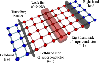
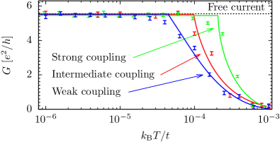
Figure 3: (Color online) Upper: The setup to model the Josephson junction. Traversing the center of the SC region is a Josephson junction (opaque cuboid). The junction is modeled by the reduction of the matrix hopping elements to $t^{\prime}=0.005$ (brown interconnects) compared to $t=1$ in the superconductor. The two metallic leads are shown in blue, and the lead-superconductor tunneling barrier by the gray cuboids. Lower: The variation of conductance with temperature for the Josephson junction. Results of the numerical computation (points) and of the theoretical model (solid lines) are shown for a weak (green), intermediate (red), and strong (blue) coupling between the two superconductors.

Another simple example that we wish to explore is a single Josephson junction, which will be modeled in the negative-$U$ Hubbard model by an intermediate region consisting of two clean superconductors, between which we insert a weak link where the nearest-neighbor hopping element $t^{\prime}$ is small ($t^{\prime}<<t$), see Fig. 3. Studying this system will allow us to probe how a phase difference across a barrier can affect the current flow through it. We again adopt a $39\%$ filled band with no disorder. We first set $t^{\prime}=0$ to disconnect the left and right-hand sides, and numerically evaluate the current through the central region. This is by no means trivial. The current formula, through the anomalous Green function, allows an absorption of a pair from the incoming lead into the condensate on one side of the barrier, and an emission of another pair into the outgoing lead. This current, however, will depend on the phase difference between the SC order parameter on the two sides of the barrier. For $t^{\prime}=0$, i.e. an infinite barrier, the phases of the left and right-hand order parameter are uncorrelated, and thus all phase differences are degenerate in energy. Therefore, the current vanishes, but only after averaging over all states, which is done automatically in our numerical procedure. In the other limit, when the hopping matrix elements are the same as the hopping through the rest of the superconductor, $t^{\prime}=t$, the phase of the superconductor is locked so we see the standard free SC current flow.

We now model the situation with a moderately sized central barrier. This splits the superconductor in two, but crucially a Josephson supercurrent flows between the two sides, thus allowing the current to flow with no additional resistance. The current $J(T)=J_{\text{J}}(T)\cos(\phi_{\text{L}}-\phi_{\text{R}})$ is maintained by the phase difference $\phi_{\text{L}}-\phi_{\text{R}}$ between the left and right-hand superconductors, and the maximum value of the dissipationless current is the critical Josephson current $J_{\text{J}}(T)=(\pi|\Delta|/2eR_{\text{n}})\tanh(|\Delta|/2k_{\text{B}}T)$ Ambegaokar63 , where $R_{\text{n}}$ is the resistance of the central barrier when the system is in the normal state.

In order to study the thermally driven disruption of the Josephson current numerically, it is vital that this breakdown occurs before the BKT transition occurs, which as we show in Sec. IV.4, by itself reduces the current flow through the system. We thus use a small hopping element for the tunneling barrier of $t^{\prime}=0.005t$, which has a large $\rho_{\text{n}}$ and therefore small Josephson current $J_{\text{J}}$. In Fig. 3 we show the current as a function of temperature, in the presence of the weak link. When there is no voltage drop across the Josephson junction, the current $J_{\text{M}}$ that flows through it is given by $J_{\text{M}}=V/R$, where $R$ is the contact resistance to the normal leads. This current is maintained as long as the critical Josephson current $J_{\text{J}}$ is larger than $J_{\text{M}}$. As temperature is increased thermal fluctuations will weaken the phase lock between the two superconducting regions, and the critical current is reduced. When $J_{\text{J}}$ is reduced below $J_{\text{M}}$, a finite voltage develops across the Josephson junction. This drives the phase difference across the junction to increase with time, which in turn leads to an oscillating current. This current has a non-zero time-average BCS , leading to a total resistance $R_{\text{JJ}}(T)=R/(1-\sqrt{1-\lambda^{2}})$, where $\lambda=J_{\text{J}}/J_{\text{M}}<1$ BCS . This time averaged current is exactly the quantity calculated in our Monte Carlo procedure. Fig. 3 depicts a comparison between this simple model and our full numerical calculation, with reasonable agreement.

The critical current can be modified by varying the resistance of the central barrier, $R_{\text{n}}$. The intermediate case has $R_{\text{n}}=0.075h/e^{2}$, the stronger coupling with $R_{\text{n}}=0.06h/e^{2}$ is obtained by lowering the barrier to $t^{\prime}=0.01t$, and the weaker coupling with $R_{\text{n}}=0.085h/e^{2}$ by widening the original barrier ($t^{\prime}=0.005t$) to four lattice sites. This wider barrier weakens the coupling between the superconductors so the Josephson resistance emerges at a lower temperature. A lower barrier strengthens the coupling so raises the temperature required for the emergence of resistance. Both these regimes are consistent with our simple model. We also verified that at very strong coupling where the temperature required for the breakdown of phase coherence becomes of the order of the BKT transition temperature our simple model for the current flow no longer captures the full physics of the system. This study validates that our formalism can correctly model the presence of the Josephson supercurrent across the weak link introduced into the superconductor, and can therefore be used to model mesoscopic systems that contain multiple SC grains.

IV.3 Decoherence and dephasing

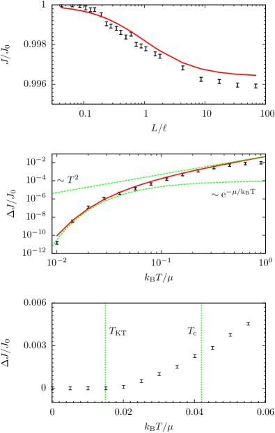
Figure 4: (Color online) (a) The relative fall in current in a one-dimensional sample due to the introduction of self energy at $k_{\text{B}}T=0.1\mu$. The black points show the numerical results, and the red line highlights the expected theoretical variation with length Micklitz10 , where $J_{0}$ is the current that flows when impeded solely by the contact resistance. (b) The relative change ($\Delta J\equiv J_{0}-J$) in current as a function of temperature in a one-dimensional normal phase sample. The black points show the numerical results, and the red the expected model variation. The two green dashed lines show the $\exp(-\mu/k_{\text{B}}T)$ and $T^{2}$ behavior. (c) The changing current in the presence of a SC phase in a two-dimensional sample. The vertical green dashed lines show the BKT and normal phase transitions.

The issue of decoherence and dephasing plays a significant role in transport at low temperatures. Here we define decoherence as the many-body phenomenon that leads to the loss of coherence via interactions among the electrons or interactions with the environment. On the other hand, dephasing can occur in a non-interacting system, and emerges from the fact that due to the finite temperature, electrons possess a range of energies, of the order of $k_{\text{B}}T$. Electrons of different energies acquire different phases along their respective trajectories, and if these phases differ by $2\pi$ or more when their energy changes by $k_{\text{B}}T$, then interference phenomena will average out to zero.

Decoherence: The effects of decoherence due to electron-electron interactions are more profound in one-dimensional wires in the normal phase. Since the original Hubbard model employed in this calculation (Eqn. (9)) is an interacting model, one expects decoherence to arise naturally from the calculation. However, though the original formula for the current is exact, the approximation employed above – Eqn. (13) – does not include quantum fluctuations. This means that it neglects the imaginary component of the self energy which corresponds to damping due to interactions, and the resulting decoherence. In order to test the effects of such decoherence due to many-body interactions, we introduce into the normal Green function for momentum $k$ (as here we study a wire in the normal phase), by hand, the self energy

$$\lim_{\delta\to 0}\frac{U^{2}}{2\pi^{4}}\sum_{\mathbf{p},\mathbf{q}}\frac{n(\xi_{\mathbf{p}})[1-n(\xi_{\mathbf{p}-\mathbf{q}})][1-n(\xi_{\mathbf{k}+\mathbf{q}})]}{\omega+\xi_{\mathbf{p}}-\xi_{\mathbf{p}-\mathbf{q}}-\xi_{\mathbf{k}+\mathbf{q}}-\text{i}\delta}\,,$$ (14)

which is the lowest order contribution to the single-particle self-energy, and where $\xi_{\mathbf{p}}$ are the momentum energy eigenstates of the Hamiltonian.

A similar approach Micklitz10 has been applied to interacting electrons in a continuous one-dimensional system with repulsive contact interactions (the second order contribution to the self-energy does not depend on the sign of the interaction). In this case, it has been shown, for wires with parabolic dispersion and chemical potential $\mu$, that this damping leads to a change in the distribution function and reduction in the conductivity by a factor of $1-\pi^{2}(k_{\text{B}}T/\mu)^{2}L/12[L+\ell\exp(\mu/k_{\text{B}}T)]$ Micklitz10 , where the wire length, $L$, is long enough that the smearing of the Fermi surface due to scattering (that occurs over the relaxation length scale $\ell$ Micklitz10 ) outweighs that due to temperature. For sufficiently long wires $L\gg\ell\exp(\mu/k_{\text{B}}T)$ the reduction in conductivity becomes length independent $1-\pi^{2}(k_{\text{B}}T/\mu)^{2}/12$.

In order to be able to compare to this theory (which relies on the parabolic dispersion), we focus on a system with a low filling fraction of $20\%$, near the bottom of the band, and set the disorder to $W=0.1t$. We employ the perturbative expression for the current, Eqn. (6), to give us access to long wires with $L\gg\ell$. In the upper panel of Fig. 4 we show the fall in current, as a function of length, due to the inclusion of self energy at $k_{\text{B}}T=0.07\mu$, here $\ell\approx 27a$. The overall change of $\sim 0.5\%$ is small due to the Pauli blocking of scattering processes near the Fermi energy. We see reasonable agreement with the model over a range of length scales. The middle panel of Fig. 4 depicts the change in current with temperature for a system of a fixed length. We highlight the agreement to the expected variation in the fall in conductance with temperature Micklitz10 . At low temperatures ($k_{\text{B}}T\ll\mu$) the damping is severely Pauli blocked so the characteristic damping length-scale exceeds the system length and the current correction $1-\pi^{2}(k_{\text{B}}T/\mu)^{2}\exp(-\mu/k_{\text{B}}T)L/12\ell$ is exponentially suppressed. As temperature increases the Fermi liquid $T^{2}$ behavior starts to dominate the correction to the current. At high, usually unphysical temperatures ($k_{\text{B}}T\gg\mu$), numerics see a smaller current shift than predicted by theory as the details of the specific Hubbard band dispersion versus the parabolic dispersion in which the model was developed become important.

In Fig. 4(c) we examine the effect of a SC phase on decoherence. At low temperature the presence of the SC gap suppresses many-body scattering processes. However, when temperature is raised above the BKT phase transition, scattering events are possible, though have a smaller impact on the current than in the normal phase, due to the still finite local pair correlations. Above the mean-field BCS phase transition the current follows the expected parabolic profile as in the normal phase. Thus we have demonstrated that while quantum fluctuations, as they affect decoherence, can be taken into account in our formalism, their effect on the current, for the range of parameters studies here, is usually small at $\lesssim 1\%$. We are thus justified in neglecting them in this study.

Figure 5: (Color online) The fall in conductance with length in a non-interacting one-dimensional wire with disorder $W=0.2t$ at two different temperatures. The red trend lines show a linear drop off in conductance with length, and green an exponential decay.

Dephasing: Having observed decoherence in the sample we now turn to study dephasing due to thermal averaging. To verify that our formalism captures this important phenomenon, we study the length dependence of the conductance in non-interacting systems. We first verified, for a non-interacting clean system, that the net macroscopic current increases by $2e^{2}/h$ for each new conduction channel introduced (not shown), independent of length. Setting the amplitude of the disorder to $W=0.2t$ and working at $39\%$ filling, in Fig. 5 we show the fall in conductance with length at two different temperatures. At $T=0$ there is an initial linear fall in conductance over length scales smaller than the localization length $\xi\approx 93a$, and an exponential fall at greater lengths. This is in accordance with the expectations of Anderson localization Ong01 – for length scales below the localization length, the conductance changes as a power law of the length, while it decays exponentially when the length becomes larger than the localization length. At $k_{\text{B}}T=0.01t$, on the other hand, dephasing causes different parts of the system to be incoherent with respect to the others, causing the conductance to fall linearly with inverse length, as expected from a classical system. This observation confirms that the formalism naturally incorporates the physics of dephasing in disordered systems.

IV.4 Variation of resistance with temperature

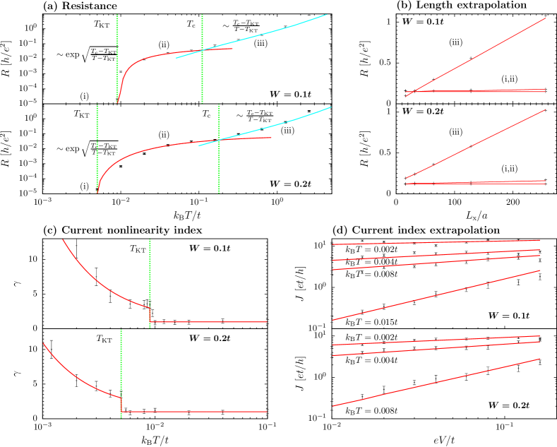
Figure 6: (Color online) (a) The variation of resistance with temperature for two different values of disorder calculated numerically (points). The red solid line shows the theoretical low temperature behavior, and the blue solid line the theoretical high temperature behavior. The dashed vertical green lines show the BKT $T_{\text{KT}}$ and mean-field $T_{\text{c}}$ temperatures. (b) The numerical results (black points) and the deduced linear length dependence (red line) of the resistance for three different points (i) $T<T_{\text{KT}}$, (ii) $T_{\text{KT}}<T<T_{\text{c}}$, and (iii) $T>T_{\text{c}}$. (c) The current nonlinearity index $\gamma$ in $V\propto J^{\gamma}$ for two disorder levels, as a function of temperature. The black points are the numerical results and the red lines are from theory. The vertical green dashed line highlights the BKT transition temperature. (d) Examples of the numerical measurements of dimensionless current against voltage leading to the values of $\gamma$ shown in the left-hand plot. The best-fit lines employed are shown in red.

We have now verified that our formalism captures the basic phenomena of contact resistance in Sec. IV.1, Josephson coupling in Sec. IV.2, and dephasing and decoherence in Sec. IV.3. With these key tests complete, we are now ideally poised to study further effects within the superconductor, starting with the temperature dependence of the conductivity and its relation to the BKT transition. With increasing temperature a two-dimensional superconductor undergoes a BKT transition Kosterlitz73 characterized by the emergence of vortices across the system, leading to the loss of global phase coherence. At a higher (“mean-field”) temperature, the SC order is completely suppressed and the system loses the SC correlation even locally. To study how this transition is reflected in the current flow we performed numerical simulations on a two-dimensional $39\%$ filled SC system at several different temperatures. Simulations were performed for two different levels of disorder, $W=0.1t$ and $W=0.2t$, to determine how the transition and current flow are modified by the normal-state resistance, and extrapolated over length to remove the effects of the contact resistance (Fig. 6(b)).

Even at temperatures below the BKT transition, vortices can be nucleated from the edge of the sample and traverse the system, driven by the Magnus force due to the finite current. This produces dissipation at any non-zero temperature and current $J$, according to the non-linear potential $V\propto J^{1+2T_{\text{KT}}/T}$ Halperin79 . In Fig. 6(a) we see that below the BKT temperature the linear resistance, that is $\lim_{V\to 0}V/J$, is zero. The plots Fig. 6(d) show several simulations that were performed for different imposed potential differences $V$ across the sample, which allowed us to extract the index $\gamma$ of the conductance relation $V\propto J^{\gamma}$. In Fig. 6(c) we show that the conductance relation approximately follows the expected theoretical behavior with $\gamma=1+2T_{\text{KT}}/T$.

At temperatures above the BKT transition vortices and anti-vortices can easily unbind, though they may be partially pinned by disorder. The finite conductance $G$ of a sample in this case has been shown by Halperin and Nelson Halperin79 to be given by

$$G=0.37G_{\text{n}}(\xi_{+}/\xi_{\text{c}})^{2}\,,$$ (15)

where $G_{\text{n}}$ is the normal state conductance, $\xi_{\text{c}}$ is the SC coherence length, and $\xi_{+}$ is the SC order correlation length, which diverges at $T_{\text{KT}}$. The critical behavior at temperatures near the BKT transition $T\gtrsim T_{\text{KT}}$ leads to the conductance

$$G=0.37G_{\text{n}}b^{-1}\exp[\sqrt{b(T_{\text{c}}-T_{\text{KT}})/(T-T_{\text{KT}})}]\,,$$ (16)

where $b$ is a number of order unity. At temperatures higher than the (renormalized) mean-field critical temperature $T_{\text{c}}$, the conductance is given by the Aslamasov-Larkin theory Aslamasov68 ; Halperin79

$$G=0.37G_{\text{n}}(T_{\text{c}}-T_{\text{KT}})/(T-T_{\text{KT}})\,.$$ (17)

Finally, we can also estimate the crossover between these two regimes by noting that the difference between the Kosterlitz-Thouless and mean-field transition temperatures critical regime is given by Halperin79

$$T_{\text{c}}-T_{\text{KT}}\approx 0.17e^{2}T_{\text{c}}/\hbar\sigma_{\text{n}}\,.$$ (18)

The difference between these two temperatures therefore widens with falling normal state conductance.

In Fig. 6(a) we depict the variation of resistance with temperature above the BKT transition, showing the two types of dependence on temperature as is expected by theory. We also note that the rising disorder increases the normal state resistance $\sigma_{\text{n}}$, and also broadens the difference between the Kosterlitz-Thouless and mean-field transition temperatures, which agrees with Eqn. (18) within $~{}20\%$. The high temperature Aslamasov-Larkin expression for the conductance persists well above the the mean-field critical temperature, where the SC state has been totally suppressed. Finally, when the temperature is of the same order as the bandwidth, $k_{B}T\sim t$, the resistance in Fig. 6(a) increases superlinearly as the Fermi distribution becomes smeared across the whole band structure.

Figure 7: (Color online) (a) The nonlinear $J-V$ characteristic of a one-dimensional superconductor at fixed temperature. The numerical points are shown with black error bars and the Langer-Ambegaokar-McCumber-Halperin model Langer67 ; McCumber70 by the red line. (b) The variation of resistance with temperature for fixed bias. The numerical points are shown with black error bars and the Langer-Ambegaokar-McCumber-Halperin model by the red line.

Having studied the nonlinear $J-V$ characteristic in two dimensions we now turn to look at the one dimensional system. Here thermal fluctuations can drive the formation of phase slips at any temperature and so this system has the $J-V$ characteristic $V=J_{0}R\sinh(J/J_{0})$ Langer67 ; McCumber70 ; Altomare05 , where $J_{0}=4ek_{\text{B}}T/h$ and $R=(h/4e^{2})\times(\hbar\Omega/k_{\text{B}}T)\exp(-\Delta F/k_{\text{B}}T)$ is the resistance with attempt frequency $\hbar\Omega\approx 3.1t$ and energy barrier $\Delta F\approx 3.7t$. In Fig. 7(a) we show the consistency of the numerical model both for the nonlinear $J-V$ characteristic, and in Fig. 7(b) the variation with temperature. The strong accord between analytics and numerics in both one and two dimensions gives us confidence that the formalism can be applied to study and explore less well understood mesoscopic superconducting systems.

IV.5 Little-Parks effect

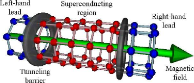
Figure 8: (Color online) Upper: A schematic of the cylindrical wire within the negative-$U$ Hubbard model. The left and right-hand metallic leads are shown in blue, from which electrons can tunnel through the gray toroids into the central SC region which is shown in red. The magnetic flux threading the cylinder is shown in green. Lower: The variation of current with longitudinal magnetic flux at $T=T_{\text{c}}$. The computational points with error bars are shown in black, and the Little-Parks model best fit is shown by the red dashed line.

Varying an applied magnetic field has long been an important experimental probe of the properties of a superconductor. It is therefore imperative to verify that the current formula developed here, coupled with the Hubbard model for the superconductor, is able to accurately model the effects of an applied magnetic field. In the Hubbard model the effects of the magnetic field are incorporated, via the Peierls substitution, into the phases of the hopping elements, $t_{ij}\rightarrow t_{ij}\text{e}^{2\pi\text{i}\phi_{ij}/\phi_{0}}$ where $\phi_{0}=hc/e$ is the quantum flux, and the phases $\phi_{ij}$ are defined such that their integral over a closed trajectory is equal to the magnetic flux threading the surface spanned by the trajectory.

In order to check whether this procedure captures the effect of an orbital magnetic field, we apply it to a hollow cylindrical superconductor, of radius $r$, such as that shown in Fig. 8, threaded by magnetic flux. As demonstrated by Little and Parks Little62 , the flux suppresses superconductivity and the transition temperature falls periodically with the flux. This is often probed by measuring the falling conductance of the cylinder near to the transition temperature Little62 ; Liu01 .

We apply our formalism to the cylindrical thin-walled superconductor shown in Fig. 8 at $39\%$ filling and no disorder, and apply an external magnetic flux $\phi$ along the axis of the cylinder. The additional phase shift to the hopping matrix elements around the cylinder circumference causes the energy of electrons in the cylinder of radius $r$ to increase with trapped flux $\phi$ as $\hbar^{2}(n+2\phi/\phi_{0})^{2}/2mr^{2}$, where the integer $n$ is chosen to minimize the energy. This results in a periodic parabolic variation of the electron energy with flux and thus a parabolic periodic oscillation in the SC transition temperature $\Delta T_{\text{c}}=\hbar^{2}(n+2\phi/\phi_{0})^{2}/16mr^{2}$ Little62 . Therefore, for a cylinder held just below its superconducting transition temperature, with increasing flux the superconducting state is disrupted periodically and the resistance varies with flux, as a series of parabolas, with minima in the conductance at every half flux quantum $\phi=n\phi_{0}/2$. This has indeed been observed experimentally Little62 .

In Fig. 8 we take a cylinder held near to its SC transition temperature and numerically evaluate the conductance as a function of the magnetic flux. The reasonable agreement with theory demonstrates that the formalism correctly picks up the effects of an applied magnetic field. The deviation from the parabolic predictions of mean-field theory at every half flux quantum is due to thermal fluctuations, and will elaborated upon in a later publication.

IV.6 Current distribution maps

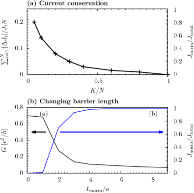
Figure 9: (Color online) (a) The average fractional error in conservation of current $\sum_{i=1}^{N}|\Delta J_{i}|/J_{i}N$ on each site against the fraction of total states $K/N$ included in the calculation of the current. (b) The changing conductance (black line) with width $L_{\text{norm}}$ of central normal region, the right axis shows the normal fraction $J_{\text{norm}}/J_{\text{total}}$ of the total current (blue line) flowing through the central region.

(a) Current map for a short barrier $L_{\text{norm}}=a$

(b) Current map for a long barrier $L_{\text{norm}}=4a$

  

Figure 10: (Color online) The upper panel shows the potential difference $V(x)$ across the sample with total potential drop $V$. The lower panel shows current maps for short (a) and long barriers (b) respectively. Supercurrent is shown by cyan darts and normal current by violet pointers, arrow length corresponds to current magnitude and orientation to the direction of current flow. Color density corresponds to the order parameter $|\Delta|$, which has peak value $\Delta_{0}$.

(a) Superconductor-insulator transition

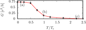
(b) SC side of transition, $T\approx 0.14T_{\text{c}}$

(c) At the superconductor-insulator transition, $T\approx T_{\text{c}}$

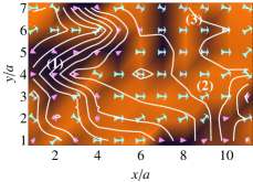
(d) Insulating side of transition, $T\approx 2.3T_{\text{c}}$

  

Figure 11: (Color online) (a) Shows the fall in conductance across the superconductor-insulator transition. Current maps on tuning temperature from (b) a superconductor at $T\approx 0.14T_{\text{c}}$ through to (d) an insulator at $T\approx 2.3T_{\text{c}}$. At $T\approx T_{\text{c}}$ the superconductor-insulator transition takes place. Supercurrent is shown by cyan darts and normal current by violet pointers, arrow length corresponds to current magnitude and orientation to the direction of current flow. Color density corresponds to the order parameter $|\Delta|$. Lines of equal chemical potential are shown in white. In the current map (b) three points of interest are labeled: (1) the normal state, (2) the superconductor state, and (3) Josephson tunneling.

One important feature of our formalism is the new capability to map out the flow of both super and normal currents within a sample and the changes in chemical potential which drive that flow. Since we can now study the current flow around impurities in the sample and expose weak links with large potential drop, we should be able to probe phenomena in the disordered superconductor with unprecedented detail and trace their cause back to a microscopic mechanism. While applications of this formalism to the outstanding problems in this field will be described in future publications, in this section we aim to demonstrate the usefulness of the current and potential maps, first by further studying the Josephson junction with a superconductor containing a central normal region, and secondly by studying the superconductor-insulator transition in disordered systems. However, we will first verify our current mapping formalism by examining the site-by-site current conservation in a $39\%$ filled system with no disorder. As the only sources and sinks of current are the two metallic leads, a consistent calculation should obey charge conservation for all of the inner sites of the sample. In Fig. 9(a) we show the average fractional error in conservation of current $\sum_{i=1}^{N}|\Delta J_{i}|/J_{i}N$ on each site as we vary the number of states $K$ included in the calculation out of a possible $N$ states, as prescribed in the penultimate paragraph of App. B. We see that if only $5\%$ of states are included there is a $20\%$ average leakage of the current. However, if we include $50\%$ of the states in the calculation of the current there is a leakage of only $\sim 2\%$. Throughout the remainder of this section we include $40\%$ of the states in the calculation to yield an average error of approximately $3\%$.

Having verified the conservation of current, we demonstrate what can be learned from the current maps by first studying a modified Josephson setup consisting of two clean $39\%$ filled SC regions with a central normal region that has $U=0$. We can then monitor the current flow through the system to see it change from SC to normal in character as the intermediate normal region is widened in Fig. 9(b). For a narrow $U=0$ central region the two SC regions are phase locked and predominantly a Josephson current flows (lower panel in Fig. 10(a)). Due to the strong proximity effect, the system is entirely SC with no reduction in conductance. The electrical potential is dropped on the two contact barriers, and remain constant through the superconductor (upper panel in Fig. 10(a)). (For the present case of two equal contact barriers the potential in the SC is equal to the average of the chemical potential of the two leads). On the other hand, when the central $U=0$ region is wide, $L_{\text{norm}}\gtrsim 4a$, the two SC regions are too weakly coupled for a Josephson current to flow, and instead a normal current flows between the two SC regions (lower panel in Fig. 10(b)). This, in turn, introduces a new resistor into the sample and the conductance drops accordingly. Now the potential drop is mostly across the Josephson junction (upper panel in Fig. 10(b)) – the left-hand superconductor adopts, approximately, the potential of the left-hand lead and the right-hand superconductor that of the right-hand lead. This situation is analogous to current flowing between SC grains in a disordered sample, and can reveal whether they are coherently coupled, when a supercurrent flows between the grains, or decoupled, when a normal current flows. Such analysis could be a vital component in the study of the origin of resistance in disordered SC system, and will be used in a subsequent publication, to study the anomalous magnetoresistance observed in experiment Sambandamurthy04 .

We give a glimpse of such an analysis in the case of the superconductor-insulator transition in a disordered superconductor with increasing temperature. We take a $39\%$ filled model with weak disorder, set to $W=0.2t$, which displays a superconductor-insulator transition at a temperature $T_{\text{c}}\approx 0.14t$. In Fig. 11(a) we show the variation of conductance across the superconductor-insulator transition, and below it study the current distribution maps. In Fig. 11(b) at $T\approx 0.14T_{\text{c}}$ there are weak-disorder driven fluctuations in the SC order parameter, but an almost uniform supercurrent. The potential drops mainly in the contacts, and in the sample is equal to the average of the two leads with small random fluctuations. In Fig. 11(d) at $T\approx 2.3T_{\text{c}}$ the SC order parameter practically vanishes, there is no supercurrent, and, due to the increasing resistance, only a small normal current flows through the sample. The potential, as expected for normal systems, decays linearly across the sample. At intermediate temperatures $T\approx T_{\text{c}}$ the current map Fig. 11(c) highlights the interplay of the normal and SC current. There is a rough correlation between regions of finite SC order parameter and supercurrent flow, on one hand, and zero SC order parameter and normal current, on the other. We point out three typical regions of the sample. Firstly, at (1) the order parameter is small and only normal current flows, whereas at (2) the order parameter is large and supercurrent flows. However, at (3) two SC regions are separated by a small normal region but are Josephson coupled and so a supercurrent flows through the zero SC order region. By examining the potential lines we see that the normal regions, for example (1), are acting as weak links whereas the potential drop over the superconducting regions is small. Thus the overall resistance of the sample is dominated by such weak links. The current and potential maps allow us to see the superconductor-insulator transition developing, and we plan to investigate in details the relation of such a percolative picture to the Kosterlitz-Thouless transition, as was recently suggested Erez2010 .

V Discussion

In this paper we have developed a new exact formula to calculate the current through a superconductor connected to two non-interacting metallic leads with an imposed potential difference. The formula was implemented with a negative-$U$ Hubbard model which included both phase and amplitude fluctuations in the SC order parameter. A new Chebyshev expansion method allowed us to solve the model and calculate the current in $\mathcal{O}(N^{1.9}M^{2/3})$ time, granting access to systems of unprecedented size. The formalism also enables the generation of current and potential maps which show exactly where the super current and separately the normal current flows through the system.

The formalism was exhaustively tested against a series of well-established results, demonstrating the accuracy of the procedure, its ability to capture various physical processes relevant to superconductivity in disordered systems, and correctly model the presence of a magnetic field and finite temperature. These tests indicate that the formalism and accompanying numerical solver can robustly calculate the current through a superconductor across a wide range of systems. In the future we plan to report on the application of the formalism to several outstanding questions, such as the magneto-resistance anomaly on crossing the superconductor-insulator transition Sambandamurthy04 , the Little Parks effect in nano-scale cylinders Liu01 , and dissipation-driven phase transitions in SC wires Lobos09 .

Acknowledgments: GJC acknowledges the financial support of the Royal Commission for the Exhibition of 1851, the Kreitman Foundation, and National Science Foundation Grant No. NSF PHY05-51164. This work was also supported by the ISF.

Appendix A Derivation of the Current Formula

The formula for the current in the Bogoliubov basis set is

$$J\!=\!\frac{\text{i}e}{2h}\!\sum_{\sigma}\!\int\!\!\text{d}\epsilon\Bigl{(} \!\!\operatorname{Tr}\!\left\{\!\left[f_{\text{L}}(\epsilon)\mathsf{\Gamma}^{\text{L}}\!-\!f_{\text{R}}(\epsilon)\mathsf{\Gamma}^{\text{R}}\right]\!\left[\mathbf{u}_{i}\!\left(\mathsf{G}_{\sigma}^{>}\!-\!\mathsf{G}_{\sigma}^{<}\right)\!\mathbf{u}_{j}^{*}\!+\!\mathbf{v}_{i}\!\left(\mathsf{G}_{-\sigma}^{>}\!-\!\mathsf{G}_{-\sigma}^{<}\right)\!\mathbf{v}_{j}^{*}\!-\!\sigma\mathbf{v}_{i}^{*}\!\left(\mathsf{H}_{\sigma}^{>}\!-\!\mathsf{H}_{\sigma}^{<}\right)\!\mathbf{u}_{j}^{*}\!+\!\sigma\mathbf{u}_{i}\!\left(\bar{\mathsf{H}}_{-\sigma}^{>}\!-\!\bar{\mathsf{H}}_{-\sigma}^{<}\right)\!\mathbf{v_{j}}\right]\!\right\}$$

$$+ \operatorname{Tr}\left\{\left[\mathsf{\Gamma}^{\text{L}}-\mathsf{\Gamma}^{\text{R}}\right]\left[\mathbf{u}_{j}^{*}\mathsf{G}^{<}_{\sigma}\mathbf{u}_{i}^{*}-\mathbf{v}_{j}\mathsf{G}^{>}_{-\sigma}\mathbf{v}_{i}^{*}+\sigma\mathbf{u}^{*}_{j}\mathsf{H}_{\sigma}^{>}\mathbf{v}^{*}_{i}-\sigma\mathbf{v}_{j}\bar{\mathsf{H}}_{-\sigma}^{<}\mathbf{u}_{i}\right]\right\}\Bigr{)}\,.$$ (19)

We need to determine the Green functions across the sample, which must be calculated in the presence of the leads. However, as the electrons in the metallic leads are non-interacting we can start from the bare electronic Green functions for the superconductor not coupled to the leads $\tilde{G}^{\text{r}}_{\text{e}\sigma}(m,n)=\delta_{m,n}/(\epsilon-\xi_{m}+\text{i}\delta)$ and $\tilde{G}^{\text{r}}_{\text{h}\sigma}(m,n)=\delta_{m,n}/(\epsilon+\xi_{m}+\text{i}\delta)$, which have energy eigenstates $\xi_{m}$ and $\delta\to 0^{+}$. We then write down Dyson’s equation to self-consistently include the leads

$$\left(\begin{array}[]{c}\mathsf{G}^{\text{r}}_{\sigma}\\ \mathsf{H}^{\text{r}}_{\sigma}\end{array}\right)=\left(\begin{array}[]{c}\mathsf{\tilde{G}}^{\text{r}}_{\text{e}\sigma}\\ 0\end{array}\right)+V^{2}\left(\begin{array}[]{cc}\mathsf{\tilde{G}}^{\text{r}}_{\text{e}\sigma}(\mathbf{u}_{\mathbf{p}}^{*}g^{\text{r}}_{\text{e}\mathbf{p}\chi}\mathbf{u}_{\mathbf{p}}+\mathbf{v}_{\mathbf{p}}^{*}g^{\text{r}}_{\text{h}\mathbf{p}\chi}\mathbf{v}_{\mathbf{p}})&\sigma\mathsf{\tilde{G}}^{\text{r}}_{\text{e}\sigma}(\mathbf{v}^{*}_{\mathbf{p}}g^{\text{r}}_{\text{h}\mathbf{p}\chi}\mathbf{u}_{\mathbf{p}}^{*}-\mathbf{u}_{\mathbf{p}}^{*}g^{\text{r}}_{\text{e}\mathbf{p}\chi}\mathbf{v}^{*}_{\mathbf{p}})\\ \sigma\mathsf{\tilde{G}}^{\text{r}}_{\text{h}\sigma}(\mathbf{u}_{\mathbf{p}}g^{\text{r}}_{\text{h}\mathbf{p}\chi}\mathbf{v}_{\mathbf{p}}-\mathbf{v}_{\mathbf{p}}g^{\text{r}}_{\text{e}\mathbf{p}\chi}\mathbf{u}_{\mathbf{p}})&\mathsf{\tilde{G}}^{\text{r}}_{\text{h}\sigma}(\mathbf{u}_{\mathbf{p}}g^{\text{r}}_{\text{h}\mathbf{p}\chi}\mathbf{u}_{\mathbf{p}}^{*}+\mathbf{v}_{\mathbf{p}}g^{\text{r}}_{\text{e}\mathbf{p}\chi}\mathbf{v}^{*}_{\mathbf{p}})\end{array}\right)\left(\begin{array}[]{c}\mathsf{G}^{\text{r}}_{\sigma}\\ \mathsf{H}^{\text{r}}_{\sigma}\end{array}\right)\,.$$ (28)

Here $g_{\text{e}\mathbf{p}\chi}^{\text{r}}=1/(\epsilon-\varepsilon_{\mathbf{p}}+\mu_{\chi}+\text{i}\delta)$ is the retarded Green function of the non-interacting electrons in the leads, with dispersion $\varepsilon_{\mathbf{p}}$, and $\{\mathsf{u}_{\mathbf{p}},\mathsf{v}_{\mathbf{p}}\}$ are the matrices of the eigenstates multiplied by the lead plane wave states $\mathbf{p}$ at the tunneling barriers. To extract the retarded Green function and its anomalous counterpart from this matrix equation one has to perform a matrix inversion. The Dyson equation is for the retarded and advanced Green functions, whereas the current formula Eqn. (19) is in terms of the lesser and greater Green functions. To transform these into the retarded and advanced Green functions we apply the identity $\mathsf{G}_{\sigma}^{<}=\tilde{\mathsf{G}}_{\sigma}^{<}+\tilde{\mathsf{G}}_{\sigma}^{\text{r}}\mathsf{\Sigma}_{\sigma}^{\text{r}}\mathsf{G}_{\sigma}^{<}+\tilde{\mathsf{G}}_{\sigma}^{\text{r}}\mathsf{\Sigma}_{\sigma}^{<}\mathsf{G}_{\sigma}^{\text{a}}+\tilde{\mathsf{G}}_{\sigma}^{<}\mathsf{\Sigma}_{\sigma}^{\text{r}}\mathsf{G}_{\sigma}^{\text{a}}$ recursively to find $\mathsf{G}_{\sigma}^{<}=(1+\mathsf{G}_{\sigma}^{\text{r}}\mathsf{\Sigma}_{\sigma}^{\text{r}})\tilde{\mathsf{G}}_{\sigma}^{<}(1+\mathsf{\Sigma}_{\sigma}^{\text{a}}\mathsf{G}_{\sigma}^{\text{a}})+\mathsf{G}_{\sigma}^{\text{r}}\mathsf{\Sigma}_{\sigma}^{<}\mathsf{G}_{\sigma}^{\text{a}}$, where $\mathsf{\Sigma}_{\sigma}$ is the self energy. This recursion fixes the chemical potential of the superconductor by including tunneling to and from the leads. This will ensure that the net number of electrons is conserved, analogous to some extensions to the BTK formalism Lambert91 . However, as the final chemical potential must be independent of the chemical potential of the uncoupled superconductor, the term containing $\tilde{\mathsf{G}}^{<}$ must be identically zero leaving $\mathsf{G}^{<}_{\sigma}=\mathsf{G}^{\text{r}}_{\sigma}\mathsf{\Sigma}^{<}_{\sigma}\mathsf{G}^{\text{a}}_{\sigma}$, and its greater Green function counterpart $\mathsf{G}^{>}_{\sigma}=\mathsf{G}^{\text{r}}_{\sigma}\mathsf{\Sigma}^{>}_{\sigma}\mathsf{G}^{\text{a}}_{\sigma}$. We now extend this identity to include the anomalous Green function and recover

$$\left(\begin{array}[]{c}\mathsf{G}^{<}_{\sigma}\\ \mathsf{H}^{<}_{\sigma}\end{array}\right)=V^{2}\left(\begin{array}[]{cc}\mathsf{G}^{\text{r}}_{\sigma}(\mathbf{u}_{\mathbf{p}}^{*}g^{<}_{\text{e}\mathbf{p}\chi}\mathbf{u}_{\mathbf{p}}+\mathbf{v}^{*}_{\mathbf{p}}g^{<}_{\text{h}\mathbf{p}\chi}\mathbf{v}_{\mathbf{p}})&\sigma\mathsf{G}^{\text{r}}_{\sigma}(\mathbf{v}^{*}_{\mathbf{p}}g^{<}_{\text{h}\mathbf{p}\chi}\mathbf{u}^{*}_{\mathbf{p}}-\mathbf{u}^{*}_{\mathbf{p}}g^{<}_{\text{e}\mathbf{p}\chi}\mathbf{v}^{*}_{\mathbf{p}})\\ \sigma\mathsf{H}^{\text{r}}_{\sigma}(\mathbf{u}_{\mathbf{p}}g^{<}_{\text{h}\mathbf{p}\chi}\mathbf{v}_{\mathbf{p}}-\mathbf{v}_{\mathbf{p}}g^{<}_{\text{e}\mathbf{p}\chi}\mathbf{u}_{\mathbf{p}})&\mathsf{H}^{\text{r}}_{\sigma}(\mathbf{u}_{\mathbf{p}}g^{<}_{\text{h}\mathbf{p}\chi}\mathbf{u}^{*}_{\mathbf{p}}+\mathbf{v}_{\mathbf{p}}g^{<}_{\text{e}\mathbf{p}\chi}\mathbf{v}^{*}_{\mathbf{p}})\end{array}\right)\left(\begin{array}[]{c}\mathsf{G}^{\text{a}}_{\sigma}\\ \mathsf{H}^{\text{a}}_{\sigma}\end{array}\right)\,.$$ (35)

We can now take this, the analogous expression for the greater Green function, and their anomalous counterparts, and substitute them into Eqn. (19), which will yield Eqn. (4).

Appendix B Evaluation of the Monte Carlo Integrals

Figure 12: (Color online) (a) The estimate of the current with number of Monte Carlo iterations, $i$, out of a total number $I=1000$. The primary y-axis shows the best estimate of the current (blue). The secondary y-axis shows the estimated standard deviation in this estimate (green) and idealized improvement in the accuracy (red). (b) The distribution of 50 separate current estimates at $T=0$ (red) and $T=0.2T_{\text{c}}$ (green) with best-fit Gaussian distributions. (c and d) The time $\tau$ to perform a run on a $32\times 32$ system renormalized by the time $\tau_{0}$ for a $M=512$, $N=1$ system. In (c) the change with varying the system size $N$, where the blue line is for the standard $\mathcal{O}(N^{4})$ method of finding all of the energy eigenvalues, the green is the $\mathcal{O}(N^{2})$ standard Chebyshev expansion method Weisse09 , and the blue is the $\mathcal{O}(N^{1.9})$ extended Chebyshev approach. In (d) the two Chebyshev expansion method approaches are compared by varying the expansion order $M$. As in (c), the green line is the standard $\mathcal{O}(M)$ approach Weisse09 , and the red line is the new $\mathcal{O}(M^{2/3})$ algorithm.

In order to evaluate the correlation functions (e.g. Eq. 13), we need to sum over all possible spatial configurations of the auxiliary fields $\bm{\rho}$ and $\{\bm{\Delta},\bar{\bm{\Delta}}\}$, with each configuration carrying the weight $P(\bm{\rho},\bm{\Delta})=\exp(-\beta E[\bm{\rho},\bm{\Delta}])/\mathcal{Z}$. This distribution is sampled using the Metropolis algorithm Metropolis53 , which at each step proposes a new configuration of either the field $\bm{\rho}$ or $\bm{\Delta}$ and calculates the resulting change in the total energy. If this change in the energy is negative the step is accepted, whereas if positive it is accepted with probability $\exp\{-\beta(E[\bm{\rho}_{\text{new}}]-E[\bm{\rho}_{\text{old}}])\}$ and $\exp\{-\beta(E[\bm{\Delta}_{\text{new}}]-E[\bm{\Delta}_{\text{old}}])\}$ respectively. Since the walk over $\bm{\rho}$ is one-dimensional we choose the step size $|\bm{\rho}_{\text{new}}-\bm{\rho}_{\text{old}}|$ to aim for $50\%$ of the steps to be accepted, whereas the walk over $\{\bm{\Delta},\bar{\bm{\Delta}}\}$ covers a two-dimensional space so we choose a step size $|\bm{\Delta}_{\text{new}}-\bm{\Delta}_{\text{old}}|$ so that $35.2\%$ of the steps will be accepted Gelman96 .

Central to the Monte Carlo method used to sample the partition function is the requirement to calculate the energy difference between two different configurations of the auxiliary fields, $\{\bm{\rho}_{\text{old}},\bm{\Delta}_{\text{old}}\}$ and $\{\bm{\rho}_{\text{new}},\bm{\Delta}_{\text{new}}\}$. For a lattice with $N$ sites, to calculate the energy of each proposed configuration requires an effort of $\mathcal{O}(N^{3})$, so an entire sweep over the $N$ sites that make up the fields $\bm{\rho}$ and $\{\bm{\Delta},\bar{\bm{\Delta}}\}$ requires a computational effort of $\mathcal{O}(N^{4})$. However, a recent method developed by Weiße Weisse09 calculates just the difference between the energy of the configurations in a computationally efficient manner. For an update to the $i\text{th}$ site a Chebyshev expansion with the $0\leq m\leq M$ coefficients containing $\langle i|\mathsf{T}_{m}(\hat{H}/s)|i\rangle$ must be calculated, where $\mathsf{T}_{m}$ is defined by the recursion relation $\mathsf{T}_{m}(\mathsf{x})=2\mathsf{x}\mathsf{T}_{m-1}(\mathsf{x})-\mathsf{T}_{m-2}(\mathsf{x})$, $\mathsf{T}_{0}(\mathsf{x})=\mathsf{I}$, and $\mathsf{T}_{1}(\mathsf{x})=\mathsf{x}$. A typical expansion contained $M=1024$ terms. Previous authors Weisse09 have calculated this site-by-site through a succession of sparse matrix-vector multiplications, each of cost $\mathcal{O}(NM)$, so for an entire sweep over the order parameter the computational effort is $\mathcal{O}(N^{2}M)$. However, here we optimize the programme so that the entire sweep can be performed in $\mathcal{O}(N^{1.9}M^{2/3})$ time. Rather than follow a site-by-site approach calculated with sparse matrix-vector multiplications we instead calculate the matrix elements for the entire sweep simultaneously, which necessitates performing matrix-matrix multiplications. Provided the changes in the order parameters are small the local changes are independent of those of surrounding sites and we can then perform the entire sweep from this data set. Spherical averaging further reduces the influence of changes in the surrounding order parameters. Central to the recursion relation for $\mathsf{T}_{m}$ is the costly calculation of $\mathsf{x}^{n}$, for $1<n\leq M$. To evaluate this we divide the calculation of the $M$ matrix products into three stages:

1. The lowest order matrix products, up to $\mathsf{x}^{k}$, are sparse. Therefore, for the elements $1<n\leq k$ the matrix multiplications involve only sparse matrices, each of peak cost $kN$, and the total cost of calculating them is $\mathcal{O}(k^{2}N)$.

2. The second stage is to successively calculate every $k\text{th}$ matrix product. Each of these involves multiplying the dense matrix $\mathsf{x}^{pk}$ by the matrix $\mathsf{x}^{k}$, for integer $1\leq p\leq M/k$, which costs $\mathcal{O}(N^{2.38})$ time Coppersmith90 . With $M/k$ of these products to calculate the total cost is $\mathcal{O}(N^{2.38}M/k)$.

3. The third stage is to construct the entire family of $\mathsf{x}^{n}$ by interpolating between the matrices $\mathsf{x}^{pk}$ found in the second stage. This is done by multiplying the dense matrices found in the second stage by the sparse matrices found in the first stage. Furthermore, as we need only the diagonal elements of the final matrix each separately costs $\mathcal{O}(kN)$ and so the total cost is $\mathcal{O}(kNM)$.

Having now laid out the prescription of how to calculate the matrix elements, we now examine the total cost, $\mathcal{O}(k^{2}N+N^{2.38}M/k+kNM)$. The choice $k\sim\sqrt[3]{N^{1.38}M}$ will minimize the total cost to $\mathcal{O}(N^{1.9}M^{2/3}+N^{1.46}M^{4/3})$, and as typically $N\gg M$ the cost is $\sim\mathcal{O}(N^{1.9}M^{2/3})$. This is a significant improvement over the cost $\mathcal{O}(N^{2}M)$ of the Chebyshev expansion approach Weisse09 , which for the parameters employed in our simulations corresponds to a speedup by a factor of $\sim 30$. Now that the matrix elements behind the Chebyshev expansion have been found they are applied for the entire sweep.

To verify the Monte Carlo procedure in Fig. 12(a) we first check the convergence of the estimate for the current and that its standard error falls as the root of the number of Monte Carlo iterations. In Fig. 12(b) we compare the results of equilibrated Monte Carlo runs at zero temperature from a variety of initial configurations of the order parameter fields $\rho$ and $\Delta$. Evolution under the Metropolis algorithm drives these starting fields into different relaxed configurations, which because the simulations are restricted here to $T=0$ are unable to be excited out to explore different configurations. These final configurations yield a variety of different current values, with standard deviation of $\sim\pm 2.4\%$ of the final total current. At finite temperature thermal excitations can drive the system to explore configurations around the ground state with a narrower standard deviation of $\sim\pm 0.6\%$. Having verified the current statistics, in Fig. 12(c and d) we show the results of some timing runs that highlight the improvement of the algorithm to $\mathcal{O}(N^{1.9}M^{2/3})$ time over the standard approach of calculating all the energy eigenvalues in $\mathcal{O}(N^{4})$ time and the standard Chebyshev approach that runs in $\mathcal{O}(N^{2}M)$ time. In particular, by varying the system size we observe that the method of calculating all the eigenvalues is more efficient for systems smaller than $N\sim 10$, but the new Chebyshev approach is superior for large systems. We took advantage of this development to study systems of unprecedented size.

The Chebyshev expansion method just described represents a zero order approximation. However, we can extend this method further and calculate the lowest order change in the Chebyshev expansion following a shift in the configuration of the fields $\bm{\rho}$ and $\bm{\Delta}$ by $\bm{\delta}$. The resultant shift in the Chebyshev expansion of $\mathsf{T}_{i}$ is found using the recursion relationships $\mathsf{t}_{i}=\frac{2}{s}\bm{\delta}\mathsf{T}_{i-1}+\frac{2}{s}\mathsf{H}\mathsf{t}_{i-1}-\mathsf{t}_{i-2}$ with $\mathsf{t}_{0}=0$ and $\mathsf{t}_{1}=\bm{\delta}/s$. This allows the Chebyshev expansion coefficients to be extrapolated over several configuration space sweeps, and the calculation time falls proportionally. Spherical averaging also reduces the influence of changes in the surrounding order parameters. In practice it was found that up to ten extrapolation steps could be performed, resulting in a code speed-up of a factor of ten.

Though the Chebyshev approach can be used to direct the sampling of the system, to calculate expectation values, such as the current, it is necessary to diagonalize the system and determine the field configurations of its states. Formally this requires $\mathcal{O}(N^{3})$ time. However, since the current is dominated by the quasiparticle states near to the Fermi surface we instead adopt the Implicitly Restarted Arnoldi Method Lehoucq96 to calculate only those particular states. We are also helped by the sparsity of the matrix, which allows us to calculate $K$ eigenstates in $\mathcal{O}(KN)$ time. It is usually necessary to calculate a certain fraction of the energy states, so $K\propto N$, and the total cost is $\mathcal{O}(N^{2})$. The eigenfunctions and energies can then be used to calculate the current for a specific realization of $\bm{\rho}$ and $\bm{\Delta}$ using the formalism described in Sec. II. It is then necessary to average over successive realizations of $\bm{\rho}$ and $\bm{\Delta}$. However, the contribution from successive Monte Carlo calculations might be serially correlated which would result in an underestimated value for the uncertainty in the predicted value of the current. To correct for this we calculated the correlation time through the truncated autocorrelation function Grotendorst02 . We find a typical correlation time of approximately six Monte Carlo steps, which without autocorrelation corrections would correspond to an underestimate in the uncertainty of a factor of $\sim 2.5$.

References

- (1) See, e.g., Superconductivity of metal and alloys, P.G. de Gennes (Addison Wessley, Redwood City, CA, 1989).
- (2) For a review, see B.I. Halperin, G. Refael and E. Demler, arXiv:1005.3347.
- (3) V.L. Berezinskii, Sov. Phys. JETP 32, 493 (1971); J.M. Kosterlitz and D.J. Thouless, Journal of Physics C: Solid State Physics, 6, 1181, (1973).
- (4) D.J. Resnick, J.C. Garland, J.T. Boyd, S. Shoemaker, and R.S. Newrock Phys. Rev. Lett. 47, 1542 (1981); D.W. Abraham, C.J. Lobb, M. Tinkham, and T.M. Klapwijk, Phys. Rev. B 26, 5268 (1982); R.F. Voss and R.A. Webb, Phys. Rev. B 25, 3446 (1982).
- (5) A.T. Fiory, A.F. Hebard, and W.I. Glaberson, Phys. Rev. B 28, 5075 (1983); A.F. Hebard and A.T. Fiory, Phys. Rev. Lett. 50, 1603 (1983); A.M. Kadin, K. Epstein, and A.M. Goldman, Phys. Rev. B 27, 6691 (1983); H. Teshima, K. Ohata, H. Izumi, K. Nakao, T. Morishita, and S. Tanaka, Physica C, bf 185-189 1865 (1991); Ali Yazdani, W.R. White, M.R. Hahn, M. Gabay, M.R. Beasley, and A. Kapitulnik, Phys. Rev. Lett. 70, 505 (1993).
- (6) A.K. Pradhan, S.J. Hazell, J.W. Hodby, C. Chen, Y. Hu, and B.M. Wanklyn, Phys. Rev. B 47, 11374 (1993); Z. Sefrioui, D. Arias, C. Leon, J. Santamaria, E.M. Gonzalez, J.L. Vicent, and P. Prieto, Phys. Rev. B 70, 064502 (2004); J.M. Repaci, C. Kwon, Qi Li, Xiuguang Jiang, T. Venkatessan, R.E. Glover, C.J. Lobb, and R.S. Newrock, Phys. Rev. B 54, R9674 (1996); V.A. Gasparov, Low Temp. Phys. 32, 838 (2006).
- (7) T. Wang, K.M. Beauchamp, A.M. Mack, N.E. Israeloff, G.C. Spalding, and A.M. Goldman, Phys. Rev. B 47, 11619 (1993); V.F. Gantmakher, M.V. Golubkov, V.T. Dolgopolov, G.E. Tsydynzhapov and A.A. Shashkin, JETP Lett. 68, 363 (1998); G. Sambandamurthy, L.W. Engel, A. Johansson, and D. Shahar, Phys. Rev. Lett. 92, 107005 (2004).
- (8) G. Sambandamurthy, L.W. Engel, A. Johansson, E. Peled, and D. Shahar, Phys. Rev. Lett. 94, 017003 (2005); V.M. Vinokur, T.I. Baturina, M.V. Fistul, A. Yu. Mironov, M.R. Baklanov and C. Strunk, Nature 452, 613 (2008).
- (9) N. Reyren, S. Thiel, A.D. Caviglia, L. Fitting Kourkoutis, G. Hammerl, C. Richter, C.W. Schneider, T. Kopp, A.-S. Rüetschi, D. Jaccard, M. Gabay, D.A. Muller, J.-M. Triscone, and J. Mannhart, Science 317, 1196 (2007); A.D. Caviglia, S. Gariglio, N. Reyren, D. Jaccard, T. Schneider, M. Gabay, S. Thiel, G. Hammerl, J. Mannhart, and J.-M. Triscone, Nature 456, 624 (2008); J. Biscaras, N. Bergeal, A. Kushwaha, T. Wolf, A. Rastogi, R.C. Budhani, and J. Lesueur, Nature Comm. 1, 1084 (2010).
- (10) A.Rufenacht, J.-P. Locquet, J. Fompeyrine, D. Caimi and P. Martinoli, Phys. Rev. Lett. 96, 227002 (2006); D. Matthey, N. Reyren, J.-M. Triscone, and T. Schneider, Phys. Rev. Lett. 98, 057002 (2007); I. Hetel, T.R. Lemberger, and M. Randeria, Nature Phys. 3, 700 (2007).
- (11) G.E. Blonder, M. Tinkham and T.M. Klapwijk, Phys. Rev. B 25, 4515 (1982).
- (12) I.O. Kulik, Sov. Phys. JETP 30, 944 (1970).
- (13) C.J. Lambert, J. Phys.: Condens. Matter 3, 6579 (1991); Y. Takane and H. Ebisawa, J. Phys. Soc. Jpn. 61, 1685 (1992); C.W.J. Beenakker, Phys. Rev. B 46, 12841 (1992); C.J. Lambert, V.C. Hui and S.J. Robinson, J. Phys.: Condens. Matter 5, 4187 (1993); I.K. Marmorkos, C.W.J. Beenakker and R.A. Jalabert, Phys. Rev. B 48, 2811 (1993); M.P. Anantram and S. Datta, Phys. Rev. B 53, 16390 (1996); N.M. Chtchelkatchev and I.S. Burmistrov, Phys. Rev. B 75, 214510 (2007); R. Mélin, C. Benjamin and T. Martin, Phys. Rev. B 77, 094512 (2008).
- (14) R. Landauer, IBM J. Res. Dev. 1, 233 (1957); R. Landauer, Philos. Mag. 21, 863 (1970).
- (15) M. Büttiker, Phys. Rev. Lett. 57, 1761 (1986).
- (16) O. Entin-Wohlman, Y. Imry and A. Aharony, Phys. Rev. B 78, 224510 (2008).
- (17) A.T. Dorsey, Phys. Rev. B 43, 7575 (1991).
- (18) Y.V. Nazarov and T.H. Stoof, Phys. Rev. Lett. 76, 823 (1996).
- (19) J.S. Langer and V. Ambegaokar, Phys. Rev. 164(2), 498 (1967).
- (20) D.E. McCumber and B.I. Halperin, Phys. Rev. B 1, 1054 (1970).
- (21) B.I. Halperin and D.R. Nelson, J. Low Temp. Phys. 36, 599 (1979); V. Ambegaokar, B.I. Halperin, D.R. Nelson and E.D. Siggia, Phys. Rev. B. 21, 1806 (1980).
- (22) H.P. Büchler, V.B. Geshkenbein, and G. Blatter, Phys. Rev. Lett. 92, 067007 (2004).
- (23) N. Trivedi, R.T. Scalettar, and M. Randeria, Phys. Rev. B 54, 3756 (1996).
- (24) Y. Meir and N.S. Wingreen, Phys. Rev. Lett. 68, 2512 (1992).
- (25) M. Mayr, G. Alvarez, C. Sen, and E. Dagotto, Phys. Rev. Lett. 94, 217001 (2005); Y. Dubi, Y. Meir, and Y. Avishai, Nature 449, 876 (2007).
- (26) A. Erez and Y Meir, EPL, 91, 47003 (2010).
- (27) C.J. Lambert, J. Phys.: Condens. Matter 3, 6579 (1991).
- (28) C. Caroli, R. Combescot, P. Nozieres, and D. Saint-James, J. Phys. C 4, 916 (1971).
- (29) A. Cresti, R. Farchioni, G. Grosso, and G.P. Parravicini, Phys. Rev. B 68, 075306 (2003).
- (30) A. Altland and B. Simons, Condensed Matter Field Theory, Cambridge University Press (2006).
- (31) S. De Palo, C. Castellani, C. Di Castro, and B.K. Chakraverty, Phys. Rev. B 60, 564 (1999).
- (32) N. Metropolis, M.N. Rosenbluth, A.H. Teller, and E. Teller, J. of Chem. Phys. 21, 1087 (1953).
- (33) R.T. Scalettar, E.Y. Loh, J. E. Gubernatis, A. Moreo, S.R. White, D. J. Scalapino, R.L. Sugar, and E. Dagotto, Phys. Rev. Lett. 62, 1407 (1989).
- (34) V. Ambegaokar and A. Baratoff, Phys. Rev. Lett. 10, 486 (1963).
- (35) P.G.-de-Gennes, Superconductivity of Metal and Alloys, Persues Books (1999).
- (36) T. Micklitz, J. Rech, and K.A. Matveev, Phys. Rev. B 81, 115313 (2010).
- (37) N.P. Ong and R.N. Bhatt, More is different: fifty years of condensed matter physics, Princeton University Press (2001).
- (38) J.M. Kosterlitz and D.J. Thouless, Journal of Physics C: Solid State Physics, 6, 1181, (1973).
- (39) L.G. Aslamasov and A.I. Larkin, Phys. Lett. 26A, 238 (1968).
- (40) F. Altomare, A.M. Chang, M.R. Melloch, Y. Hong, and C.W. Tu, arXiv:cond-mat/0505772 (2005).
- (41) W.A. Little and R.D. Parks, Phys. Rev. Lett. 9, 9 (1962).
- (42) Y. Liu, Y. Zadorozhny, M.M. Rosario, B.Y. Rock, P.T. Carrigan, and H. Wang, Science 294, 2332 (2001).
- (43) G. Sambandamurthy, L.W. Engel, A. Johansson, and D. Shahar, Phys. Rev. Lett. 92, 107005 (2004).
- (44) A.M. Lobos, A. Iucci, M. Müller and T. Giamarchi, Phys. Rev. B 80, 214515 (2009).
- (45) A. Gelman, G.O. Roberts and W.R. Gilks, Bayesian Statistics 5, 599 (1996).
- (46) A. Weiße, Phys. Rev. Lett. 102, 150604 (2009).
- (47) D. Coppersmith and S. Winograd, Journal of Symbolic Computation 9, 251 (1990).
- (48) R.B. Lehoucq and D.C. Sorensen, SIAM. J. Matrix Anal. & Appl. 17, 789 (1996).
- (49) J. Grotendorst, D. Marx and A. Muramatsu, Quantum Simulations of Many-Body Systems: From Theory to Algorithms, John von Neumann Institute for Computing, Jülich, NIC Series 10, 423 (2002).