Anisotropic quasiparticle lifetimes in Fe-based superconductors

Abstract

We study the dynamical quasiparticle scattering by spin and charge fluctuations in Fe-based pnictides within a 5-orbital model with onsite interactions. The leading contribution to the scattering rate is calculated from the second-order diagrams with the polarization operator calculated in the random phase approximation. We find one-particle scattering rates which are highly anisotropic on each Fermi surface sheet due to the momentum dependence of the spin susceptibility and the multi-orbital composition of each Fermi pocket. This fact combined with the anisotropy of the effective mass, produce disparity between electrons and holes in conductivity, Hall coefficient, and Raman initial slope in qualitative agreement with experimental data.

I Introduction

The presence of several electronic orbitals in bands near the Fermi level of a metallic system provides both a rich set of properties and complications in revealing the underlying physics. Some of the most widely discussed examples of such systems are the recently discovered Fe-based superconductors with $T_{c}$ up to 55K Kamihara et al. (2008); Zhi-An Ren, Wei Lu, Jie Yang, Wei Yi, Xiao-Li Shen, Zheng-Cai Li, Guang-Can Che, Xiao-Li Dong, Li-Ling Sun, Fang Zhou, Zhong-Xian Zhao (2008) where multi-orbital effects cannot be disregarded. In these quasi-two-dimensional compounds, Fe $d$-orbitals form a Fermi surface (FS) consisting of nearly compensated small electron and hole pockets.Lebègue (2007); Singh and Du (2008) Since the sizes of the hole and electron FS pockets are roughly identical in the undoped system, one might expect a vanishingly small Hall coefficient and a roughly electron-hole symmetric doping dependence. However, in the intensively studied 122 systems (Ba(Fe_1-xCo${}_{x})_{2}$As₂, Ba(Fe_1-xNi${}_{x})_{2}$As₂) and 1111 systems (LaFeAsO_1-xF_x and SmFeAsO_1-xF_x), Hall effect measurements find that transport is dominated by the electrons even for the parent compoundsRullier-Albenque et al. (2009); Fang et al. (2009); Kasahara et al. (2010); Liu et al. (2008); Riggs et al. (2009); Hess et al. (2009). In the compensated case, this result can be explained only if the mobilities of holes and electrons are remarkably different which suggests an order of magnitude disparity in relaxation times, $\tau_{e}\gg\tau_{h}$. Fang et al. (2009) A similar large asymmetry of electronic and hole scattering rates has also been suggested in the analysis of the electronic Raman measurements which can selectively probe different parts of the Brillouin zone (BZ) using various polarizations Muschler et al. (2009). Optical conductivity as measured by THz spectrometry provides and estimate of $\tau_{e}\approx 4\tau_{h}$, Maksimov et al. (2010) and reflectivity measurements also suggest the presence of two distinct scattering rates with a large disparity between them. Barisic et al. (2010); Tu et al. (2010); van Heumen et al. (2010) Theoretical analysis of the normal state resistivity $\rho$ in the two-band model for Ba_1-xK_xFe₂As₂ shows that the experimental temperature dependence $\rho(T)$ can be reproduced only if one assumes order of magnitude larger scattering in the hole band Golubov et al. (2010). Finally, quantum oscillation experiments on P-doped systems indicate that the electron pockets have a longer mean free path Analytis et al. (2010); Coldea et al. (2008); Analytis et al. (2009). It is clearly important to understand whether this conjectured dichotomy between electron and hole transport properties is real, and if it is universal to the Fe-based superconductors.

There are two main sources for quasiparticle decay: i) electron-electron inelastic processes and ii) impurity scattering. We will concentrate on the first case and mention impurity scattering only briefly. Experimentally, the apparent disparity in mobilities for holes and electrons becomes smaller as one dopes away from the magnetically ordered parent compounds Fang et al. (2009). This suggests that the spin fluctuations which also decrease upon doping play an important role in the scattering rate asymmetry. Spin fluctuations due to the nearby spin-density wave (SDW) state have also been considered as the most probable source of superconducting pairing.Mazin et al. (2008); Kuroki et al. (2008); Graser et al. (2009)

In this paper we study the inelastic quasiparticle scattering in Fe-based superconductors by calculating the scattering rate on different FS sheets within the generalized spin-fluctuation theory. The self-energy is approximated via the second-order diagrams with the polarization operator treated in the random phase approximation (RPA). We show that there are two ingredients which provide strong anisotropy of the scattering rate.

The most important one is that one-particle scattering is strongly affected by the orbital character of the initial and final states, in analogy to orbital pair scattering effects which have been discussed recently,Maier et al. (2009); Kemper et al. (2010) leading to a momentum dependence of the effective interaction. Secondly, the polarization bubble itself is momentum dependent. The combination results in a highly anisotropic scattering rate on the electron Fermi surface sheets, including some very long lived quasiparticle states. Although our results indicate that on the average $\tau_{e}$ is of the same order as $\tau_{h}$, the transport properties still may be dominated by small parts of the electron pockets where the lifetimes are long and the Fermi velocities are high. This combination causes a disparity between holes and electrons in the transport properties (conductivity and Hall coefficient). Furthermore, analysis of the Raman response shows that the quasiparticle lifetime effects can be clearly observed in both the B_1g and B_2g polarizations.

A calculation of the lifetime on Fermi surface was previously reported by Onari et al.Onari and Kontani (2010), where the scattering due to spin fluctuations was considered within the fluctuation-exchange approximation (FLEX). Our results reveal a similar momentum dependence of the lifetimes, but exhibit a much larger anisotropy due to the absence of self-consistency.

II Model

We will use the 5-orbital tight-binding model of Graser et al. Graser et al. (2009) which is based on the ab initio band structure calculations Cao et al. (2008) within the local density approximation (LDA) for the prototypical iron pnictide, LaOFeAs. Our interaction Hamiltonian is

$$H = H_{0}+U\sum_{i,m}n_{im\uparrow}n_{im\downarrow}+U^{\prime}\sum_{i,m<n}n_{in}n_{im}$$ (1)

$$+J\sum_{i,m<n}\sum_{\sigma,\sigma^{\prime}}c_{in\sigma}^{\dagger}c_{im\sigma^{\prime}}^{\dagger}c_{in\sigma^{\prime}}c_{im\sigma}$$

$$+J^{\prime}\sum_{i,m\neq n}c_{in\uparrow}^{\dagger}c_{in\downarrow}^{\dagger}c_{im\downarrow}c_{im\uparrow},$$

where $n_{im}=n_{im\uparrow}+n_{im\downarrow}$, $n_{im\sigma}=c_{im\sigma}^{\dagger}c_{im\sigma}$, with $i$, $m$, and $\sigma$ denoting site, orbital, and spin indices, respectively. The on-site intra- and inter-orbital Hubbard repulsions ($U$ and $U^{\prime}$), Hund’s rule coupling ($J$), and the pair hopping ($J^{\prime}$) correspond to the notations of Kuroki et al. Kuroki et al. (2008) Below we will consider cases which obey spin-rotation invariance (SRI) through the relations $U^{\prime}=U-2J$ and $J^{\prime}=J$ and those which do not. The kinetic energy $H_{0}$ includes the chemical potential $\mu$ and is described by a tight-binding model spanned by five Fe $d$-orbitals ($d_{\textnormal{xz}}$ , $d_{\textnormal{yz}}$ , $d_{\textnormal{x}^{2}-\textnormal{y}^{2}}$ , $d_{\textnormal{xy}}$ , $d_{3\textnormal{z}^{2}-\textnormal{r}^{2}}$ ) Graser et al. (2009). The $d_{\textnormal{xz}}$ , $d_{\textnormal{yz}}$ and $d_{\textnormal{xy}}$ bands dominate near Fermi level, as seen in Fig. 1 where we show the Fermi surface (FS) which arises from $H_{0}$ in the one-Fe Brillouin zone. For the electron- and undoped systems the FS consists of two small hole pockets $\alpha_{1}$ and $\alpha_{2}$ around the $\Gamma=(0,0)$ point, and two small electron pockets $\beta_{1}$ and $\beta_{2}$ around the $X=(\pi,0)$ and $Y=(0,\pi)$ points, respectively. Upon hole doping a new hole FS pocket, $\gamma$, emerges around $(\pi,\pi)$ point, which has been shown to strongly affect the pairing state Kuroki et al. (2009); Kemper et al. (2010).

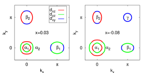
Figure 1: (Color online) Fermi surface for electron doped (doping $x=0.03$, left) and hole doped (doping $x=-0.08$, right) systems calculated within the 5-orbital model.

III Method

The leading non-vanishing contribution to the quasiparticle scattering rate $1/\tau$ comes from the imaginary part of the second-order self-energy diagram ($\mathrm{Im}\ \Sigma$) with the polarization bubble (see Fig. 2). To take scattering from spin fluctuations into account we renormalize the bubble within the random phase approximation (RPA). Note that second order diagrams with crossing interaction lines are not included in Fig. 2. We have chosen to work in this approximation to preserve consistency with calculations of the spin fluctuation pairing vertex Graser et al. (2009). The bubble then represents the RPA susceptibility which in the multi-orbital system is $\chi_{wz}^{vu}(\mathbf{q},\omega_{q})$ with $w,z,v,u$ being the orbital indices, and $\mathbf{q}$ and $\omega_{q}$ are the momentum and frequency, respectively. The same susceptibility was calculated in Ref. Graser et al., 2009 and was shown to produce superconductivity with an A_1g order parameter symmetry, in accord with several experimentsPaglione and Greene (2010) and other spin fluctuation calculations Graser et al. (2010); Kemper et al. (2010); Kuroki et al. (2008, 2009). Here and below the orbital (band) indices are denoted by Latin (Greek) letters.

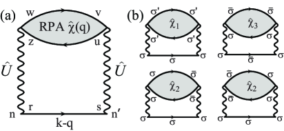
Figure 2: Orbital (a) and spin (b) structure of the second order diagram for the self-energy in the multi-orbital system, $\Sigma_{\bar{n}\bar{n}^{\prime}}(\mathbf{k},\omega)$. Interaction lines contain four orbital indices, $\hat{U}=U_{nr}^{wz}$. Shaded bubble denote the RPA susceptibility, $\hat{\chi}(q)=\chi_{wz}^{vu}(\mathbf{q},\omega_{q})$. Incoming and outgoing indices $\bar{n}$ and $\bar{n}^{\prime}$ carry the same spin $\sigma$. $\hat{\chi}_{1}$, $\hat{\chi}_{2}$, and $\hat{\chi}_{3}$ are the different susceptibility channels, see Eq. (III), $\bar{\sigma}=-\sigma$.

Since we focus on the lifetime effects, we consider only $\mathrm{Im}\ \Sigma$, neglecting the real part of the self-energy $\mathrm{Re}\ \Sigma$. The renormalization of the band structure due to the real part of the self-energy has been discussed in some detail in Refs. Ortenzi et al., 2009; Ikeda et al., 2010 and is not considered in the present study. We note that our calculations are based on the LDA band structure which already contains important Hartree corrections and agrees fairly well with quantum oscillation experiments Analytis et al. (2010); Coldea et al. (2008); Analytis et al. (2009).

There are important consequences of the multi-orbital nature of the system which deserve comment. First, the single-particle noninteracting Green function is diagonal in band space but not in orbital space. The orbital matrix elements $a_{\mathbf{k}}^{n,\lambda}$, which describe the transformation from one space to another are given by $c_{\mathbf{k}n\sigma}=\sum\limits_{\lambda}a_{\mathbf{k}}^{n,\lambda}d_{\mathbf{k}\lambda\sigma}$, where $d_{\mathbf{k}\lambda\sigma}$ is the annihilation operator for a particle with band index $\lambda$, momentum $\mathbf{k}$ and energy $\varepsilon^{\lambda}_{\mathbf{k}}$. Secondly, the interactions in Hamiltonian (1) have a complicated orbital structure; to compactify the expressions we define the local matrix interaction in orbital space, $U_{nr}^{wz}c_{iw\sigma_{1}}^{\dagger}c_{ir\sigma_{2}}^{\dagger}c_{iz\sigma_{3}}c_{in\sigma_{4}}$, which accounts for all the quartic terms.

The noninteracting part of the Hamiltonian, $H_{0}$, is a complex matrix Graser et al. (2009) which in general has complex eigenvectors $a_{\mathbf{k}}^{n,\lambda}$, although the eigenvalues $\varepsilon^{\lambda}_{\mathbf{k}}$ are real. In order to use a simple form of the spectral representation of the Green function below, we choose a gauge in which the Hamiltonian is real by performing a unitary transformation $\tilde{H_{0}}=\hat{\phi}^{-1}\hat{H}_{0}\hat{\phi}$, where $\hat{\phi}$ is the diagonal matrix $\hat{\phi}=\mathrm{diag}\left(\mathrm{i},\mathrm{i},1,1,1\right)$. The interaction part of the Hamiltonian (1) must then also be rotated by $\hat{\phi}$. Having completed the rotation, the eigenvectors and interactions are now real, and after calculating the diagram in Fig. 2 we arrive at the multi-band extension of the standard zero-temperature expressions for the self-energy:

$$\mathrm{Im}\ \Sigma_{\bar{n}\bar{n}^{\prime}}(\mathbf{k},\omega)=\sum_{\mathbf{q},\lambda}\sum_{\bar{w},\bar{z},\bar{u},\bar{v},\bar{r},\bar{s}}U_{\bar{n}\bar{r}}^{\bar{w}\bar{z}}U_{\bar{s}\bar{n}^{\prime}}^{\bar{u}\bar{v}}a^{r,\lambda}_{\mathbf{k}-\mathbf{q}}a^{s,\lambda}_{\mathbf{k}-\mathbf{q}}$$ (2)

$$\times\mathrm{Im}\ \chi_{\bar{w}\bar{z}}^{\bar{v}\bar{u}}(\mathbf{q},\omega-\varepsilon^{\lambda}_{\mathbf{k}-\mathbf{q}})\left[\Theta\left(\varepsilon^{\lambda}_{\mathbf{k}-\mathbf{q}}\right)-\Theta\left(\varepsilon^{\lambda}_{\mathbf{k}-\mathbf{q}}-\omega\right)\right].$$

For simplicity, we have introduced the notation $\bar{s}=(s,\sigma_{s})$, where $s$ and $\sigma_{s}$ are the orbital and spin index, respectively. The initial and final spins $\sigma_{n}$ and $\sigma_{n^{\prime}}$, since we are considering the paramagnetic state, have been kept equal.

The momentum dependence of the orbital matrix elements generates an effective momentum-dependent interaction from the bare local Coulomb interactions,

$$V_{\bar{n},\lambda}^{\bar{w}\bar{z}}\left(\mathbf{k}-\mathbf{q}\right)=\sum\limits_{\bar{r}}U_{\bar{n}\bar{r}}^{\bar{w}\bar{z}}a^{r,\lambda}_{\mathbf{k}-\mathbf{q}},$$ (3)

in terms of which (2) may be written

$$\mathrm{Im}\ \Sigma_{\bar{n}\bar{n}^{\prime}}(\mathbf{k},\omega)=\sum_{\mathbf{q},\lambda}\sum_{\bar{w},\bar{z},\bar{u},\bar{v}}V_{\bar{n},\lambda}^{\bar{w}\bar{z}}\left(\mathbf{q}\right)V_{\bar{n}^{\prime},\lambda}^{\bar{v}\bar{u}}\left(\mathbf{q}\right)$$ (4)

$$\times\mathrm{Im}\ \chi_{\bar{w}\bar{z}}^{\bar{v}\bar{u}}(\mathbf{k}-\mathbf{q},\omega-\varepsilon^{\lambda}_{\mathbf{q}})\left[\Theta\left(\varepsilon^{\lambda}_{\mathbf{q}}\right)-\Theta\left(\varepsilon^{\lambda}_{\mathbf{q}}-\omega\right)\right].$$

The effective interaction enhances the anisotropy of the scattering rate, as will be demonstrated below.

We now discuss briefly the spin structure of the diagram in Fig. 2 which is important for the calculation of $\mathrm{Im}\ \Sigma$ using Eq. (2). The susceptibility can be divided into charge and spin channels, and subsequently into singlet and triplet parts:

$$\chi_{\bar{w}\bar{z}}^{\bar{u}\bar{v}} =\frac{1}{2}(\chi^{c})_{wz}^{uv}\delta_{\sigma_{w}\sigma_{z}}\delta_{\sigma_{u}\sigma_{v}}+\frac{1}{6}(\chi^{s})_{wz}^{uv}\vec{\tau}_{\sigma_{w}\sigma_{z}}\cdot\vec{\tau}_{\sigma_{u}\sigma_{v}}$$

$$=\left\{\begin{array}[]{cc}\hat{\chi}_{1,2}\equiv\frac{1}{2}(\chi^{c})_{wz}^{uv}\pm\frac{1}{6}(\chi^{s})_{wz}^{uv}&\mathrm{triplet}\\ \hat{\chi}_{3}\equiv\frac{1}{3}(\chi^{s})_{wz}^{uv}&\mathrm{singlet}\end{array}\right.$$ (7)

where $\chi^{c}$ and $\chi^{s}$ are the charge and spin parts of the susceptibility, respectively, and $\vec{\tau}_{\sigma\sigma^{\prime}}$ are Pauli spin matrices.

For the purpose of the self-energy calculation, the interactions can be grouped into three channels. If we denote the incoming spins as $\sigma_{1}$ and $\sigma_{3}$, and the outgoing as $\sigma_{2}$ and $\sigma_{4}$, the channels are: (1) $\sigma_{1}=\sigma_{2}=\sigma_{3}=\sigma_{4}$, (2) $\sigma_{1}=\sigma_{2}\neq\sigma_{3}=\sigma_{4}$, (3) $\sigma_{1}\neq\sigma_{2}=\sigma_{3}\neq\sigma_{4}$. Then the orbital part of interactions in each channel, $\hat{U}_{1}$, $\hat{U}_{2}$, and $\hat{U}_{3}$, are:

$$\begin{array}[]{lll}(U_{1})_{aa}^{aa}=0&(U_{2})_{aa}^{aa}=U&(U_{3})_{aa}^{aa}=-U\\ (U_{1})_{aa}^{bb}=U^{\prime}-J&(U_{2})_{aa}^{bb}=U^{\prime}&(U_{3})_{aa}^{bb}=-J\\ (U_{1})_{ab}^{ab}=0&(U_{2})_{ab}^{ab}=J^{\prime}&(U_{3})_{ab}^{ab}=-J^{\prime}\\ (U_{1})_{ab}^{ba}=J-U^{\prime}&(U_{2})_{ab}^{ba}=J&(U_{3})_{ab}^{ba}=-U^{\prime}\end{array}$$ (12)

where orbital indices $a\neq b$.

To combine the interactions with the susceptibility, we first note that due to the spin structure of the diagram, the interaction channels (1)-(3) decouple. Second, we see by inspection that channels (1) and (2) couple to $\hat{\chi}_{1,2}$, and channel (3) couples to $\hat{\chi}_{3}$. Thus, the self-energy will contain the following matrix structure

$$\hat{U}\hat{\chi}\hat{U}\propto\hat{U}_{1}\hat{\chi}_{1}\hat{U}_{1}+\hat{U}_{2}\hat{\chi}_{1}\hat{U}_{2}+\hat{U}_{1}\hat{\chi}_{2}\hat{U}_{2}+\hat{U}_{2}\hat{\chi}_{2}\hat{U}_{1}+\hat{U}_{3}\hat{\chi}_{3}\hat{U}_{3}.$$ (13)

This expression by construction resolves the spin summation and only sums over orbital indices remain. Combining it with the calculation of $\chi_{wz}^{vu}(\mathbf{q},\omega_{q})$ for a given doping we use Eq. 2 to obtain $\mathrm{Im}\ \Sigma_{nn^{\prime}}$ straightforwardly. Then we convert it to a band representation, $\mathrm{Im}\ \Sigma_{\lambda\lambda^{\prime}}(\mathbf{k},\omega)=\sum\limits_{n,n^{\prime}}a^{n,\lambda}_{\mathbf{k}}\mathrm{Im}\ \Sigma_{nn^{\prime}}(\mathbf{k},\omega)a^{n^{\prime},\lambda^{\prime}}_{\mathbf{k}}$. For the energy range where there are no band crossings, there is a unique band $\lambda$ corresponding to the momentum $\mathbf{k}$. The self-energy describes the scattering of the particle with $\mathbf{k}$ back to the same momentum $\mathbf{k}$, and thus back to the same band, $\lambda^{\prime}=\lambda$. For the small energies around the Fermi level considered, there are no band crossings, so the major contribution to the scattering rate in the full Green function in band space, $\hat{G}=(\hat{G}_{0}^{-1}-\hat{\Sigma})^{-1}$, comes from diagonal, $\lambda=\lambda^{\prime}$, matrix elements of $\mathrm{Im}\ \hat{\Sigma}$. We denote them as $\Sigma^{\prime\prime}_{\lambda}(\mathbf{k},\omega)\equiv\mathrm{Im}\ \Sigma_{\lambda\lambda}(\mathbf{k},\omega)$. The momentum sums in Eq. 4 were performed on a 256x256 grid with an artificial broadening in all susceptibilities of 5 meV. The undoped material has completely filled d⁶ orbitals, which corresponds to $n_{e}=6$. To present our results as a function of doping, we define it as $x=n_{e}-6$.

IV Self-energy

Because inter-band transitions are negligible in the range of energies considered here, the calculated scattering rate follows the Fermi liquid relation $\Sigma^{\prime\prime}(\mathbf{k},\omega)\propto\omega^{2}+\pi^{2}T^{2}$; thus, some finite frequency or temperature is needed for non-vanishing results. Here, and below, the quantities we report will be calculated at $\omega=20$meV which is equivalent to $T\approx 74$K at zero frequency. We have verified numerically that our results scale as $\omega^{2}$, and that interband transitions indeed do not contribute at low energies. The results below are qualitatively independent of the exact frequency chosen, since we are below the range of frequencies where inter-band scattering plays a large role.

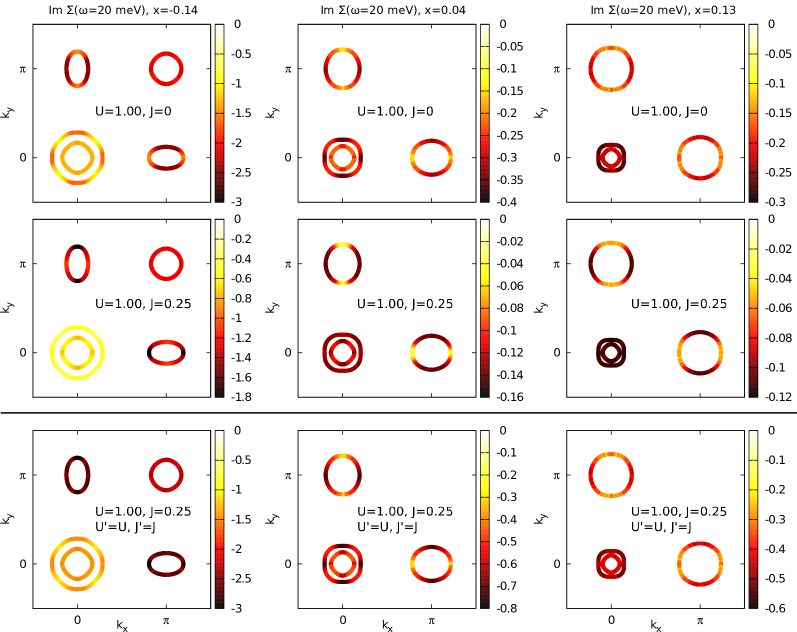
Figure 3: (Color online) Imaginary part of the self-energy $\Sigma$ at $\omega=20$meV along the Fermi surface for various dopings ($x=-0.14$, $0.04$, and $0.13$ from left to right) and for three sets of interaction parameters (in eV). All reported values are in meV. Note that the color scale is different for each plot. First and second row interaction parameters are SRI; third row is non-SRI.

For several dopings and few sets of interaction parameters, the calculated scattering rate along the Fermi surface is shown in Fig. 3. Here, $U$ and $J$ are in eV and were chosen to be close to the SDW-instability in the spin susceptibility.

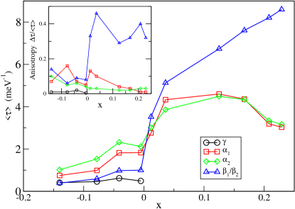
Figure 4: (Color online) Average scattering rate for holes ($\alpha_{1}$,$\alpha_{2}$,$\gamma$) and electrons ($\beta_{1}$,$\beta_{2}$) at $\omega=20$ meV and $U=1.0$ eV and $J=0.25$ eV. Inset: Lifetime anisotropy $\Delta\tau/\langle\tau\rangle$, where $\Delta\tau$ ($\langle\tau\rangle$) is the standard deviation (average) over the appropriate Fermi surface.

We observe that the average scattering rate increases monotonically with doping. Fig. 4 shows the average lifetime for holes and electrons on the Fermi surface, as well as a measure of the anisotropy which we have defined as the normalized standard deviation of the lifetime, $\Delta\tau/\langle\tau\rangle$, where $\tau_{k}=-1/2\Sigma^{\prime\prime}(k,\omega)$, scaled by the average. We see a clear increase in the quasiparticle lifetime on all Fermi surface sheets as the system is electron doped. On the electron-doped side, the average scattering rates are essentially controlled by the degree of nesting. As more electrons are doped into the system, the hole pockets shrink and the nesting between the $\alpha$ and $\beta$ sheets deteriorates. The hole-doped systems have a smaller lifetime due to the presence of the $\gamma$ pocket; in addition to $(\pi,0)$ scattering between $\alpha$ and $\beta$ sheets, new phase space for scattering opens up and the average rate increases. Since electrons on the $d_{\textnormal{xy}}$ portions of the FS are long-lived as will be discussed below, one expects the resistivity due to spin-fluctuations to increase with hole doping.

Aside from the overall change in scale, Fig. 4 shows that the ratio of electron to hole scattering rate changes as one goes from hole to electron doping; electrons have a higher average scattering rate on the hole-doped side, and vice versa. Although there is already an anisotropy between the hole and electron pockets in terms of lifetimes, it is not enough to cause the experimentally observed anisotropy, as will be discussed below. With electron doping, electron sheets $\beta_{1}$ and $\beta_{2}$ increase in size as well as $d_{xy}$ portions. Thus the number of states with long lifetime for electrons increases monotonically. On the other hand, hole pockets decrease in size and the phase space for scattering decreases, while for small pockets the intraband scattering starts to dominate. The competition of these two effects lead to saturation and then to decrease of lifetime for holes, indicating that the intraband scattering dominates.

Next, we observe a clear anisotropy in the scattering rate going around the Fermi surfaces as shown in Fig. 3 and the inset of Fig. 4. Focusing first on the undoped and electron-doped systems, the $\beta_{1}$ sheet exhibits strong anisotropy between the $\Gamma-X$ and $X-M$ directions. From Fig. 1, we observe that this is where the Fermi surface orbital composition changes from $d_{\textnormal{xy}}$ to $d_{\textnormal{yz}}$ character. There is a strong minimum in the scattering rate in the $d_{\textnormal{xy}}$ portions of the $\beta$ sheets; this is due to the above-mentioned anisotropy of the effective interaction, Eq. (3). The orbital matrix elements tend to restrict scattering to be maximal for intra-orbital processes. For the $d_{\textnormal{xy}}$ electrons, there is very little phase space to scatter compared to other orbitals, see Fig. 1, because the spin fluctuation scattering intensity $\chi(\mathbf{q})$ is peaked at $\mathbf{q}=(\pi,0)$. Thus, they behave more like free electrons. When the system is sufficiently hole doped to create the ($d_{\textnormal{xy}}$ ) $\gamma$ hole pocket, ($\pi$,0) spin fluctuations couple them strongly to other $d_{\textnormal{xy}}$ states, causing the scattering rate there to increase. Throughout the doping range, $d_{\textnormal{xz}}$ and $d_{\textnormal{yz}}$ states on the $\alpha$ pockets scatter strongly with their counterparts on the $\beta$ pockets, and vice versa.

Finally, we discuss the interaction dependence in Fig. 3. The top row of panels shows a case where $J=0$, and the middle has finite $J=0.25$. As the Hund’s rule coupling $J$ is turned on, we observe two effects. First, the overall scattering rate decreases (note that the color scale on each plot is different). This is due to the spin-rotation invariance (SRI) relation $U^{\prime}=U-2J$, so that $U^{\prime}$ is decreased in the middle row of panels. Although new scattering channels open up through $J$ itself, this is more than compensated by the decrease in the inter-orbital scattering $U^{\prime}$. This is confirmed by the third row in the figure, where $J$ is finite but the system is non-SRI because $U^{\prime}=U$, as in the first row. Here, the scattering rate increases for all dopings, indicating that it is indeed the decrease in $U^{\prime}$ that is the cause of the $\Sigma^{\prime\prime}$ decrease in the 2nd row.

Secondly, we consider the effect of $J$ on the $\beta$ sheet anisotropy for the hole-doped system. When $J=0$, the minimum scattering rate occurs near the $d_{\textnormal{xy}}$ sections of the Fermi surfaces for all dopings. Once $J$ is turned on, the anisotropy reverses, and instead a maximum scattering rate is found on the same sections. This reversal of anisotropy can be explained by the same argument as above. When $J=0$, the intra-orbital and inter-orbital scattering ($U$ and $U^{\prime}$) are the same. Thus, there is a strong scattering from both the $d_{\textnormal{xz}}$ /$d_{\textnormal{yz}}$ portions as well as the $d_{\textnormal{xy}}$ portions of the $\beta$ sheets to the $\gamma$ pocket (of $d_{\textnormal{xy}}$ character). Since the $d_{\textnormal{xz}}$ /$d_{\textnormal{yz}}$ portions additionally scatter to the $\alpha$ sheets, a stronger scattering rate occurs there. When $J$ is finite, the effective inter-orbital scattering rate $U^{\prime}$ decreases through the SRI relation. Thus, the scattering on the $d_{\textnormal{xz}}$ /$d_{\textnormal{yz}}$ portions is decreased while that on the $d_{\textnormal{xy}}$ sections remains the same. With sufficiently large $J$, the anisotropy on the $\beta$ sheets is reversed. Note, however, that this argument depends on the existence of the $\gamma$ pocket. When the pocket is not present, such as in the undoped and electron doped cases, no such reversal occurs, and thus the $d_{\textnormal{xy}}$ states have the longest lifetimes for the configurations investigated.

V Comparison with experiment

V.1 Conductivity

We next consider the effect of the calculated scattering rates on the electric conductivity. The total conductivity is the sum of the band conductivities, $\sigma(\omega)=\sum\limits_{\lambda}\sigma_{x\lambda}(\omega)$,

$$\sigma_{x\lambda}(\omega)=\frac{e^{2}}{\pi h}\int\limits_{\mathbf{k}\in\mathbf{k}_{F\lambda}}d\mathbf{k}N_{\mathbf{k}}v_{\mathbf{k}_{x}}^{2}\tau_{\mathbf{k}}(\omega),$$ (14)

where $\tau_{\mathbf{k}}=-1/2\Sigma^{\prime\prime}_{\lambda}(\mathbf{k},\omega)$, $\mathbf{k}_{F\lambda}$ is the Fermi momentum for a particular band index $\lambda$, we integrate over $\mathbf{k}_{\parallel}$ which is the component of momentum along the FS, $v_{\mathbf{k}}$ is the velocity, and $N_{\mathbf{k}_{F\lambda}}=1/|v_{\mathbf{k}_{F\lambda}}|$ is the momentum- and band-dependent density of states (DOS) at the Fermi level. Note that we have approximated the transport lifetime with the one-electron lifetime $\tau_{\mathbf{k}}$, neglecting forward scattering corrections, as well as the distinction between normal and Umklapp processes. Such an approximation can only give the crude qualitative effect of the scattering from spin fluctuations on the conductivity.

To analyze the doping-dependence of the conductivity, we now keep the interactions constant at values which do not produce an RPA instability over the range of dopings considered. We evaluate the DC conductivities at finite temperature by replacing $1/\tau_{\mathbf{k}}(\omega)$ in Eq. (14) by $1/\tau_{\mathbf{k}}(\pi T)$. It is important to ask which aspects of the doping dependence of transport arise from purely kinematic effects such as carrier density and Fermi velocity, which evolve with doping, and which arise from interactions. To illustrate this, we first plot in the top panel of Fig. 5 the separate contributions to the total conductivity from the electron and hole sheets, with an assumed constant relaxation time. Here the conductivities evolve more or less as expected with electron doping as the volumes of hole sheets shrink and electron sheets grow. On the other hand, it is important that the “perfectly compensated” situation of equal kinetic conductivity of electrons and holes does not occur for the undoped case, but rather for $x\simeq-0.05$ hole doping. We have indicated in the figure the range of doping over which the 122 systems display long range magnetic order, which is not included in the current theory, and thus where the results are not directly applicable.

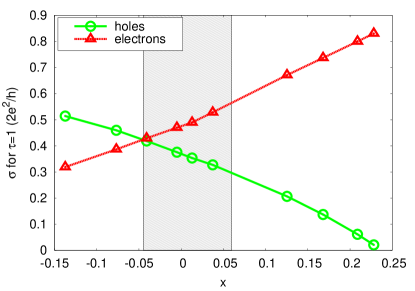
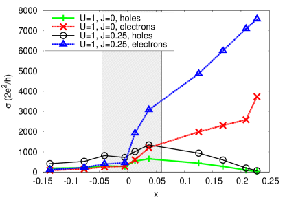
Figure 5: (Color online) Top: Conductivity for holes and electrons as a function of doping $x=n_{e}-6$ for constant relaxation rate $1/\tau=1$ eV. Bottom: conductivity for holes and electrons as a function of doping $x$ for the two sets of parameters (in eV): $U=1.0,J=0$ and $U=1.0,J=0.25$, at effective temperature $T=74K$. The shaded region marks the rough experimental SDW region in 122 systems. Solid lines are guides to the eye.

By contrast, the bottom panel of Fig. 5 shows the separate conductivities on the hole and electron FS as a function of doping. We immediately notice that conductivity for electrons grows quite strongly upon electron doping. Quite unlike the purely kinetic case in the top panel, the hole conductivity varies only weakly compared to that of the electrons. It is this asymmetry, due to a combination of the kinetic effects illustrated in the top panel of Fig. 5 and lifetime effects calculated here, which lead to the rapid domination of the conductivity by electrons; this has led transport experiments for Co-doped Ba-122 being interpreted in terms of a 1-band model with electrons only Rullier-Albenque et al. (2009); Fang et al. (2009) with some validity. The feature that greatly affects the doping dependence is the fact that the maximum of the Fermi velocity is precisely where the lifetime is largest on the electron FS sheets, namely the $d_{\textnormal{xy}}$ sections of the $\beta$ sheets. We also calculated conductivity and Hall coefficient for a case where SRI is violated ($U=1.0$, $J=0.25$, $U^{\prime}=U$, not shown in the figure). The result are qualitatively similar to the case where $U=1.0$, $J=0$.

The conductivities obtained show a large disparity between the hole- and electron-doped sides. It is important to note that what we calculate here is the spin-fluctuation contribution to the scattering rate, i.e. inelastic scattering. Resistivity experiments on K-doped and Co-doped Ba122 show that the elastic scattering is much larger in the Co-doped (e-doped) samples, presumably due to the fact that the Co dopants sit in the FeAs plane. This elastic scattering will correspondingly reduce the e-doped side of Fig.5, and thus bring the overall scattering rate more in line with the experimentally observed trends. We have not attempted to fit experiments directly due to the current uncertainty in the details of the dopant scattering potential.

The calculated conductivity shown in the lower panel of Fig. 5 was obtained for interaction parameters chosen sufficiently small to show the effect of doping while avoiding the RPA instability. For these parameters, the absolute scale of $\sigma$ is much larger than in experiments on 1111 or 122 samples. Clearly increasing the overall scale of the interactions will increase the scattering rates and decrease the conductivity. However to obtain the observed values of the conductivity requires approaching the RPA instability extremely closely. We have not attempted to fine tune the interaction strengths, but merely to illustrate the possible qualitative behavior. It seems more likely that a more complete theory will require a renormalization of the susceptibility akin to that seen in Quantum Monte Carlo (QMC) studies of the Hubbard model, which indicated that the RPA form of the dynamical magnetic response was qualitatively correct, but that the “$U$” driving the instability (through the RPA denominator) needed to be taken independent of the $U^{2}$ prefactor in the effective interaction Maier et al. (2007). A similar effect should occur in multi-orbital Hubbard models, such that the overall scales of scattering rates, and degree of proximity to the instability, should not be taken overly seriously.

V.2 Hall coefficient.

Any disparity between the scattering rates of electrons and holes manifests itself in the Hall coefficient

$$R_{H}=-\sigma_{H}(\omega)/\sigma^{2}(\omega),$$ (15)

where $\sigma_{H}(\omega)$ is the Hall conductivity Schulz et al. (1992); Kim et al. (1998). For a multi-band system, $\sigma_{H}(\omega)=\sum\limits_{\lambda}\sigma_{H\lambda}(\omega)$ and the expression for the band Hall conductivity has the form

$$\sigma_{H\lambda}(\omega)=\frac{e^{3}}{\pi h}\int\limits_{\mathbf{k}\in\mathbf{k}_{F\lambda}}d\mathbf{k}N_{\mathbf{k}}\mathbf{v}_{\mathbf{k}}\cdot\left[\mathrm{Tr}(\mathbf{M}_{\mathbf{k}}^{-1})-\mathbf{M}_{\mathbf{k}}^{-1}\right]\cdot\mathbf{v}_{\mathbf{k}}\tau_{\mathbf{k}}^{2}(\omega),$$ (16)

where $\left(\mathbf{M}_{\mathbf{k}}^{-1}\right)_{\alpha\beta}=\hbar^{-1}\partial v_{k_{\alpha}}/\partial k_{\beta}$ is the inverse mass tensor.

Fig. 6 shows calculated $R_{H}$ as a function of doping for $\omega=20$meV (the corresponding effective temperature is 74K). One can qualitatively understand the doping dependence of $R_{H}$ by analyzing the approximate equation for the band Hall conductivity,

$$\sigma_{H\lambda}(\omega)\approx R_{\lambda}\sigma_{\lambda}^{2}(\omega).$$ (17)

where $1/R_{\lambda}=\pm en_{\lambda}$ is the Hall coefficient for an electron (hole) band $\lambda$, and $n_{\lambda}$ is the occupation of that band. For the simple case of two bands (hole and electron) we have

$$R_{H}^{2band}=\frac{1}{e}\frac{\sigma_{h}^{2}/n_{h}-\sigma_{e}^{2}/n_{e}}{\left(\sigma_{h}+\sigma_{e}\right)^{2}}.$$ (18)

Since conductivity for the hole band $\sigma_{h}\propto n_{h}\tau_{h}/m_{h}$ and for the electron band $\sigma_{e}\propto n_{e}\tau_{e}/m_{e}$ with $\tau_{h,e}$ and $m_{h,e}$ being the corresponding lifetimes and band masses, $R_{H}^{2band}$ is a decreasing function of electron doping if $\tau_{e}\sim\tau_{h}$ and $m_{e}\sim m_{h}$. This is what we see in Fig. 6 for the $U=1.0,J=0$ case. On the other hand, experimental data for 1111 and 122 compounds indicate that $R_{H}^{expt}$ is an increasing function of electron doping (i.e., the magnitude $|R_{H}^{expt}|$ decreases with increasing $x$) away from the SDW state. According to the simple analysis of Eq. (18), this may be due to (i) $\tau_{e}\gg\tau_{h}$ and/or (ii) $m_{h}\gg m_{e}$. Note that use of Eq. (16) gives a different result from Eq. (17) due to the mass anisotropy across the FS which contributes to factor (ii). Factor (i) starts to play a role when we consider non-zero $J$. For the case of $U=1.0$ and $J=0.25$, $R_{H}(x)$ becomes slightly increasing function of $x$ for $x>0$ (Fig. 6). However, it is not in quantitative agreement with experimental data. To see whether the present approach can provide the correct slope of $R_{H}(x)$, we artificially increased scattering rate on all orbitals except $d_{\textnormal{xy}}$ twice, so that the anisotropy between hole and electron sheets becomes more pronounced. The resulting doping dependence of the Hall coefficient is shown in Fig. 7. Now the slope of $R_{H}(x)$ is in good agreement with experimental data.

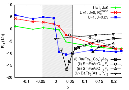
Figure 6: (Color online) Doping dependence of the Hall coefficient. The theoretical calculations are for two sets of parameters (in eV): $U=1.0$, $J=0$ and $U=1.0$, $J=0.25$. For the first set we also show result of the multi-band approximation for $R_{H}$ from Eq. (17). Experimental data points are from (i) Ref. Fang et al., 2009 for Ba(Fe_1-xCo_x)₂As₂ at 100K, (ii) Ref. Riggs et al., 2009 and (iii) Ref. Liu et al., 2008 for SmFeAsO_1-xF_x at 125K, and (iv) Ref. Kasahara et al., 2010 for BaFe₂(As_1-xP_x)₂ at 150K. The shaded region tentatively marks the experimental SDW region. Solid lines are guides for the eye.

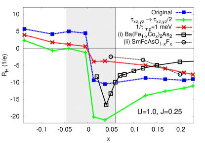
Figure 7: (Color online) Doping dependence of the Hall coefficient for three distinct cases: (1) original calculated $R_{H}$ from Fig. 6, (2) the one with the artificially increased scattering rate for all orbitals except for $d_{\textnormal{xy}}$ , $\tau_{xz,yz}\to\tau_{xz,yz}/2$, and (3) $R_{H}$ with added constant impurity scattering $1/\tau_{imp}=1$meV. For all cases parameters are $U=1.0$eV, $J=0.25$eV. Experimental data points (i) are from Ref. Fang et al., 2009 for Ba(Fe_1-xCo_x)₂As₂ at 100K. The shaded region tentatively marks the experimental SDW region. Solid lines are guides for the eye.

The fact that we underestimate the disparity between holes and electrons by a factor of two is not very discouraging. There are several factors not included in the present theory. In the interest of studying the doping dependence, we have kept the interactions fairly low to avoid the instability which occurs for relatively small interaction strengths on the hole-doped side. Furthermore, we have neglected impurity scattering. In multi-band impurity models Golubov and Mazin (1997); Senga and Kontani (2008), the ratio of intra- to inter-band scattering is taken as a parameter, and the scattering rate asymmetry between electrons and holes is weak. One might expect that an “orbital impurity” model, where an impurity introduces a local Coulomb potential for electrons in all $d$-orbitals, might produce a scattering rate anisotropy in $\mathbf{k}$-space due to the matrix elements $a_{\mathbf{k}}^{n,\lambda}$, just as in the inelastic scattering case. By investigating simple models similar to those considered in Ref. Onari and Kontani, 2009, we have concluded that both average elastic scattering rate asymmetry, and elastic scattering rate anisotropy on any given Fermi surface sheet are small. To address the effect of isotropic impurities on the Hall coefficient, we introduced a constant impurity scattering with a strength comparable to the calculated spin-fluctuation scattering rate $1/\tau_{\mathbf{k}}$. Since concurring scattering processes add to the self-energy, the scattering rate is $1/\tau_{\mathbf{k}}^{\mathrm{total}}=1/\tau_{\mathrm{imp}}+1/\tau_{\mathbf{k}}$. Substituting $\tau_{\mathbf{k}}^{\mathrm{total}}$ in Eqs. (14) and (16), we find $R_{H}(x)$ shown in Fig. 7 for $1/\tau_{\mathrm{imp}}=1$meV. Clearly, increasing disorder leads to a monotonically decreasing Hall coefficient with doping similar to Eq. 18 with $\tau_{e}\simeq\tau_{h}$. Thus dirtier samples will show a decrease of $R_{H}(x)$ with increasing electron doping.

The temperature dependence of $R_{H}$ deserves additional discussion. Recent phenomenological calculations of the self-energy in a two-band model for the pnictides suggest that to reproduce experimentally observed $R_{H}(T)$ one needs to assume the non-Fermi liquid behavior of the spin susceptibility Prelovšek and Sega (2010). In particular, for large electron dopings, $R_{H}(T)$ is almost constant but for small $x$ it become an increasing function of temperature Fang et al. (2009); Rullier-Albenque et al. (2010). Here we argue that the observed temperature dependence can be qualitatively reproduced within our Fermi liquid approach. The resulting $R_{H}(T)$ from our calculations is shown in Fig. 8. Note that the band which forms the $\gamma$ FS pocket for $x<0$ is slightly below the Fermi level for small positive $x$. Thus at finite energy or temperature the scattering to that band contributes to the self-energy and consequently to the transport properties. That is the main reason why $R_{H}(T)$ for $x=0.03$ is a rapidly changing function of $T$ in Fig. 8.

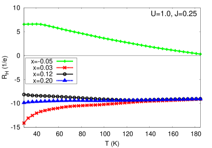
Figure 8: (Color online) Calculated dependence of the Hall coefficient on the effective temperature for several dopings $x$ with $U=1.0$eV, $J=0.25$eV.

V.3 Raman response

A momentum-sensitive probe of the scattering rate is provided by Raman spectroscopy. In particular, one can extract a scattering rate $\Gamma$ from Raman measurements by considering the slope of the Raman response in the limit as the energy loss $\Omega\rightarrow 0$. Devereaux and Hackl (2007) This quantity can be calculated as

$$\frac{1}{\Gamma_{\gamma}}= \lim_{\Omega\rightarrow 0}\frac{\partial\chi^{\prime\prime}_{\gamma\gamma}}{\partial\Omega}$$

$$= \lim_{\Omega\rightarrow 0}N_{F}^{-1}\int\limits_{\mathbf{k}\in\mathbf{k}_{F}}d\mathbf{k}\frac{N_{\mathbf{k}}\gamma_{\mathbf{k}}^{2}}{\Sigma^{\prime\prime}(\mathbf{k},\Omega)}$$ (19)

where $\gamma_{\mathbf{k}}$ denotes the Raman vertex related to the incident and scattering polarizations (see e.g. Ref. Devereaux and Kampf, 1999), and $N_{F}$ is the density of states at the Fermi level. Here, we have taken the simplest form for the Raman vertices allowed by symmetry, namely $\cos(k_{x})-\cos(k_{y})$ and $\sin(k_{x})\sin(k_{y})$ for the B_1g and B_2g channels, respectively (note that we are using the 1 Fe unit cell conventions). We do not calculate the A_1g response due to the difficulties involved in calculating the backflow effects.Devereaux et al. (1996) In general, the backflow correction to the A_1g channel involves the full susceptibility, not just the imaginary part. Although this can in principle be obtained, it is computationally expensive.

Fig. 9 shows the lifetimes obtained from Raman scattering according to the expression above.

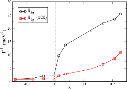
Figure 9: (Color online) Inverse of the Raman scattering rate as function of doping for $U=1.0$ eV, $J=0.25$ eV. The B_2g curve has been scaled by 20 for visibility.

As discussed in Muschler et al. Muschler et al. (2009); Mazin et al. (2010), the B_1g measurements probe the regions of the Brillouin zone containing the electron sheets. The B_2g measurements probe the region around $(\pi/2,\pi/2)$, where there nominally are no Fermi surfaces. This causes a decrease in the overall magnitude of the B_2g Raman signal compared to B_1g , as reflected in Fig. 9. However, the tails of the B_2g Raman vertex extend out to the zone edges, and thus some information can nevertheless be gleaned. On the hole doped side, the hole pockets are large, and the B_2g vertex probes the edges of the hole pockets. Similarly, when the system is electron doped, the electron pockets grow and the B_2g vertex is thus larger there. The numerator of Eq. 19 would give a symmetric doping dependence; therefore, the strong asymmetry is due to the lifetime effects.

We observe that the presence of the $\gamma$ pocket has a large effect in the Raman response, for the same reasons as in the conductivity above. In particular the B_1g signal shows a large increase around zero doping. In the B_2g channel the effect is not as strong, since there sections of both hole and electron sheets are probed.

VI Conclusions

We have shown that the quasiparticle scattering due to spin-fluctuations in a multi-orbital model with local interactions can be significantly anisotropic. Two factors which produce this effect are the orbital matrix elements, which make interactions effectively momentum-dependent, and the momentum dependence of the dynamic susceptibility. In the particular case of our model for LaOFeAs, the $d_{\textnormal{xy}}$ portions of the electron FS experience little scattering due to the small scattering phase space in undoped and electron-doped cases, since there are no $d_{\textnormal{xy}}$ states on the hole sheets available for scattering. This anisotropy on the electron sheets appears to have profound consequences for transport in at least some Fe-pnictide systems. We have noted that there are several factors which together determine the experimentally observed disparity between holes and electrons. The first is the longer lifetime of the $d_{\textnormal{xy}}$ states on the electron FS sheets. Another is the fact that the maximum of the Fermi velocity is precisely where the lifetime for electrons is largest.

Our calculations suggest that we underestimate slightly the asymmetry between $d_{\textnormal{xy}}$ and $d_{\textnormal{xz}}$ /$d_{\textnormal{yz}}$ states seen in the analysis of the Hall coefficient doping-dependence. We have discussed and critically analyzed factors which can provide additional anisotropy. Finally, we discussed aspects of the the electronic Raman scattering rate, and showed that the lifetime effects should be visible in both the B_1g and B_2g channels in varying amounts.