Impact of spin-orbit coupling on the Holstein polaron

Abstract

We utilize an exact variational numerical procedure to calculate the ground state properties of a polaron in the presence of a Rashba-like spin orbit interaction. Our results corroborate with previous work performed with the Momentum Average approximation and with weak coupling perturbation theory. We find that spin orbit coupling increases the effective mass in the regime with weak electron phonon coupling, and decreases the effective mass in the intermediate and strong electron phonon coupling regime. Analytical strong coupling perturbation theory results confirm our numerical results in the small polaron regime. A large amount of spin orbit coupling can lead to a significant lowering of the polaron effective mass.

I Introduction

In much of condensed matter (magnetism excepted), the spin and orbital components of an electron are treated as independent degrees of freedom. Nonetheless, the non-relativistic approximation to the Dirac equation leads directly to the so-called Thomas term in the effective Hamiltonian, which can be written as a spin-orbit coupling term.sakurai67 This coupling can play a significant role in the electronic structure of semiconductors and metals, as documented, for example, in Ref. (winkler03, ). More recently, interest has grown because of the burgeoning possibilities in the so-called field of spintronics, where the spin degree of freedom is specifically exploited for potential applications.wolf01 Control of spin will require coupling to the orbital motion, and hence spin-orbit coupling may play a critical role in understanding and exploiting various properties of such systems.

Spin-orbit coupling, as described by Rashba,rashba60 is expected to be prominent in two dimensional systems that lack inversion symmetry, including surface states. Many such systems have now been identified, among which are, for example, surface alloys, Li/W(110),rotenberg99 Pb/Ag(111),pacile06 ; ast07a and Bi/Ag(111).ast07b In all of these systems the possibility of other interactions remains; in particular recent workcappelluti07 has focussed on the electron-phonon interaction, in the presence of Rashba spin-orbit interactions. In the first reference of Ref. (cappelluti07, ), for example, the effective mass due to the electron-phonon interaction was shown, in weak coupling, to be enhanced by the spin-orbit interaction.

More recently, attention has focussed on the properties of a single electron interacting with oscillator degrees of freedom holstein59 in the presence of Rashba spin-orbit coupling.covaci09 These authors utilized the so-called momentum average (MA) approximationberciu06 to examine the properties of a single polaron also in the presence of spin-orbit coupling, but for a tight-binding model. They found that the effective mass generally decreases as a function of spin-orbit coupling, $V_{\mathrm{S}}$; however, in the weak electron-phonon coupling limit, there is initially an increase in effective mass, in agreement with Cappelluti et al. cappelluti07 The primary purpose of this work is to present exact solutions to this problem, using Trugman’s method,trugman90 ; bonca99 along with some modified algorithms,li10 so that we can span the entire parameter regime. It turns out that the MA method is fairly accurate over the entire parameter range, except for low phonon frequency.

We also develop a strong coupling expansion, based on the Lang-Firsov transformation,lang63 following Ref. (marsiglio95, ). As in the straightforward Holstein model, strong coupling describes fairly well the small polaron regime. Finally, the adiabatic limit of the Holstein model with Rashba spin-orbit coupling has been described recently in Ref. (grimaldi10, ), following Refs. (lagendijk85, ) and (kabanov93, ) for the simple Holstein model. In the strict adiabatic limit Grimaldi finds an intermediate state (large polaron) with the lowest energy, for coupling strengths just below that required for small polaron formation, in the presence of spin-orbit coupling (see Figs. 1 and 2 in Ref. (grimaldi10, )). Our search for this state will also be described in the present work.

The paper is organized as follows. We first introduce the model of study; following Ref. (covaci09, ) it is the Holstein model with additional Rashba spin-orbit coupling, written for a tight-binding formulation. We note some of the features of the non-interacting (with respect to phonons) model. Unlike the continuum limit,cappelluti07 there is not a singularity at the bottom of the band; however, for weak spin-orbit coupling, a singularity remains very close by in energy, and causes a significant enhancement in the density of states at the bottom of the band. In Section III we present our numerical results, along with those from the strong coupling expansion and from the MA approximation. As mentioned above, the exact numerical results confirm the conclusions from Ref. (covaci09, ). Finally, we examine the low phonon frequency and intermediate electron-phonon and spin-orbit coupling regimes, where both perturbative and MA approaches are suspect. We are unable to rule out the presence of an intermediate phase completely, but find that its occurrence is unlikely, once quantum fluctuations are included. We close with a summary.

II Model

The standard formulation for spin-orbit interaction uses two different types of electronic band structure. The first is free electron-like, which results in parabolic bands,cappelluti07 and the second is tight-binding, which results in a periodic momentum dependence. While it is essentially always the case that the latter tends to the former for low electron fillings, this is not quite true when a Rashba-type spin-orbit interaction term is present. As shown in Ref.[cappelluti07, ], for example, the ground state for a single electron consists of a degenerate ring around the $\Gamma-$point. This results in an electronic density of states with a square-root singularity at the bottom of the band. For a tight-binding model, however, Covaci et al. covaci09 pointed out that this is not the case. We will adopt a tight-binding formulation here, and examine this difference more closely in the next sub-section.

To study the single polaron with spin-orbit interaction we use a tight-binding Hamiltonian with Rashba-type spin-orbit interactionrashba60 and a Holstein-typeholstein59 electron-phonon interaction. In real space the Hamiltonian is:

$$H = -t\sum_{<i,j>,\alpha=\uparrow\downarrow}(c_{i,\alpha}^{\dagger}c_{j,\alpha}+c_{j,\alpha}^{\dagger}c_{i,\alpha})$$ (1)

$$+V_{S}\sum_{i,\alpha,\beta}(ic_{i,\alpha}^{\dagger}\sigma_{x}^{\alpha\beta}c_{i+\hat{y},\beta}-ic_{i,\alpha}^{\dagger}\sigma_{y}^{\alpha\beta}c_{i+\hat{x},\beta}+h.c.)$$

$$-g\omega_{E}\sum_{i,s=\uparrow\downarrow}c_{i,s}^{\dagger}c_{i,s}(a_{i}+a_{i}^{\dagger})+\omega_{E}\sum_{i}a_{i}^{\dagger}a_{i},$$

where $c_{i,s}^{\dagger}$ ($c_{i,s}$) is the creation (annihilation) for an electron at site $i$ with spin index $s$, $a_{i}^{\dagger}$ ($a_{i}$) is the creation (annihilation) operator for a phonon at site $i$, and $\sigma_{x}^{\alpha\beta},\sigma_{y}^{\alpha\beta}$ designate the $(\alpha,\beta)$ component of the usual Pauli matrices. The sum over $i$ is over all sites in the lattice, whereas $<i,j>$ means only nearest neighbor hopping is included. Here, as the notation already suggests, we confine ourselves to nearest neighbor hopping only. The energy scales are the hopping integral $t$, the strength of the Rashba spin-orbit interaction, $V_{S}$, the coupling of the electron to the oscillator degrees of freedom $g\omega_{E}$, and the Einstein phonon frequency, $\omega_{E}$. In what follows we write all energy scales in terms of the hopping integral, $t$, which hereafter is set to unity. The ground-state properties of the Holstein model in one and two dimensions near the adiabatic limit have recently been studied in Refs. (li10, ) and (alvermann10, ). Normally spin is not considered, since this ground state is degenerate with respect to spin. As the Rashba spin-orbit interaction is turned on, however, the two-fold degeneracy will be lifted.

II.1 non-interacting model: ground state and effective mass

To examine this model in detail, we use a $2\times 2$ matrix to describe the spin sector, and begin by excluding the phonon part of the Hamiltonian. The remaining Hamiltonian is diagonalized through Bloch states in momentum space, written as

$$H_{0}=\sum_{\mathbf{k},\alpha}\epsilon_{\mathbf{k}}c_{\mathbf{k},\alpha}^{{\dagger}}c_{\mathbf{k},\alpha}+\sum_{\mathbf{k},\alpha,\beta}\mathbf{\Omega}_{\mathbf{k}}\mathbf{\cdot\sigma}_{\alpha\beta}c_{\mathbf{k},\alpha}^{{\dagger}}c_{\mathbf{k},\beta}$$ (2)

where $\epsilon_{\mathbf{k}}=-2t[\cos(k_{x})+\cos(k_{y})]$ and $\mathbf{\Omega}_{\mathbf{k}}\mathbf{\cdot\sigma}=$ $2V_{S}[\sin(k_{y})\sigma_{x}-\sin(k_{x})\sigma_{y}]$ (we set the lattice spacing $a$ equal to unity). Diagonalizing this $2\times 2$ matrix, we get two bands, which we name the upper and lower Rashba bands. The eigenvalues and eigenstates are given by

$$H_{0}\Psi_{\pm}=\varepsilon_{k,\pm}\Psi_{\pm},$$ (3)

with eigenvalues

$$\varepsilon_{k,\pm}=-2t[\cos(k_{x})+\cos(k_{y})]\pm 2V_{S}\sqrt{\sin^{2}(k_{y})+\sin^{2}(k_{x})},$$ (4)

and eigenvectors

$$\Psi_{\pm}=\frac{1}{\sqrt{2}}\left[c_{k\uparrow}^{\dagger}\pm\frac{\sin(k_{y})-i\sin(k_{x})}{\sqrt{\sin^{2}(k_{y})+\sin^{2}(k_{x})}}c_{k\downarrow}^{\dagger}\right]|0\rangle.$$ (5)

In contrast to the model with parabolic bands, this model has a four-fold degenerate ground state located at $k_{x}=k_{y}=\pm\arctan(\frac{V_{S}}{\sqrt{2}t})$,covaci09 which can be seen clearly from a contour plot of the lower Rashba band in Fig.1. There are also four saddle points near the energy minimum points, which are located at $k_{x}=0,k_{y}=\pm\arctan(\frac{V_{S}}{t})$ and $k_{y}=0,k_{x}=\pm\arctan(\frac{V_{S}}{t})$. As $V_{S}$ increases, the separation between minimum points and saddle points is enhanced (see below, in Fig.2(b)).

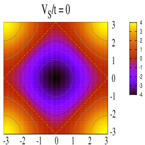
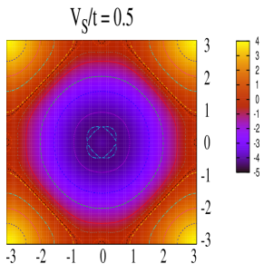
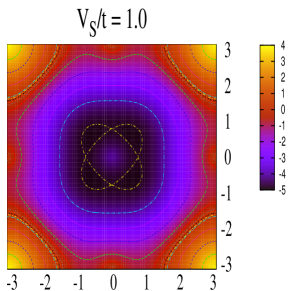
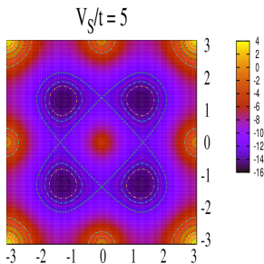
Figure 1: (color online) Contour plots for lower Rashba band with $V_{S}/t=0,0.5,1.0,5.0$. For $V_{S}=0$, there is only one energy minimum point at $k_{x}=k_{y}=0$. For $V_{S}>0$, there are four energy minimum points located at $k_{x}=k_{y}=\pm\arctan(\frac{V_{S}}{t\sqrt{2}})$. For nonzero $V_{S}$, there are also four saddle points near the energy minimum points, which are located at $k_{x}=0,k_{y}=\pm\arctan(\frac{V_{S}}{t})$ and $k_{y}=0,k_{x}=\pm\arctan(\frac{V_{S}}{t})$. As $V_{S}$ increases, the separation between minimum points and saddle points is increased (see Fig.2(b)).

The ground state energy for $H_{0}$ is given by $E_{0}=-4t\sqrt{1+V_{S}^{2}/(2t^{2})}$. Similarly, the effective mass along the diagonal is

$$\frac{m_{\mathrm{SO}}}{m_{0}}=\frac{1}{\sqrt{1+V_{S}^{2}/(2t^{2})}},$$ (6)

where $m_{0}\equiv 1/(4t)$ is the bare mass in the absence of spin-orbit interaction, and $m_{\mathrm{SO}}$ is the effective mass due solely to spin-orbit interaction. Note that the effective mass decreases due to spin-orbit interaction. Below we will turn on the electron phonon interaction, and the ground state energy (effective mass) will be further lowered (raised) due to polaronic processes.

II.2 non-interacting model: electron density of states

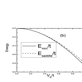
Figure 2: (a) Non-interacting density of states $D_{-}(E)$ near the bottom of the band for $V_{S}/t=0,0.5,1.0$. In the inset the density of states in the whole band is shown for the same parameters. Note that the divergence at the bottom of the band has been shifted to higher value.covaci09 (b) The separation between energy minimum points and saddle points as a function of spin orbit interaction $V_{S}/t$.

The non interacting electron density of states (DOS) is defined for each band, as

$$D_{s}(E)=\sum_{k}\delta(E-\epsilon_{ks})$$ (7)

with $s=\pm 1$.

In the main frame of Fig.2(a) we show the low energy DOS for various values of the spin orbit interaction $V_{S}$; note that this involves only $D_{-}(E)$ as the upper Rashba band exists only at higher energies. Furthermore, information concerning the upper Rashba band can always be obtained through the symmetry

$$D_{+}(E)=D_{-}(-E).$$ (8)

Fig.2(a) shows that a divergence introduced by the spin orbit interaction exists at higher energy,covaci09 and not at the bottom of the band, as occurs for a parabolic dispersion.cappelluti07 This shift is due to the separation of the energy minima from the saddle points in k-space, as shown in Fig.2(b). The saddle point energy is given by $E_{\rm sad}=-2t(1+\sqrt{1+({V_{S}/t})^{2}})$, which is very close to the minimum energy $E_{0}$ even for sizeable $V_{S}/t$, as is evident from the figure. This proximity of the divergence serves to elevate the value of the DOS at the bottom of the band. With no spin orbit coupling this value is $D_{\pm}(E=E_{0}=-4t)=1/(4\pi t)$ ($V_{S}=0$). With spin orbit coupling, however, an expansion around the minimum energy $E_{0}=-4t\sqrt{1+V_{S}^{2}/2t^{2}}$ yields a DOS value

$$D_{-}(E=E_{0})={\sqrt{2}\over\pi}{1\over V_{S}}\phantom{aaaaa}V_{S}\neq 0.$$ (9)

Thus a discontinuity occurs as the spin orbit coupling is changed from zero — the DOS immediately has a divergence at the bottom of the band which, for any non-zero value of $V_{S}$, shifts to slightly higher energy. The inset shows $D_{-}(E)$ over a wider energy range. Further details are provided in Appendix A.

III Ground state energy and effective mass

When the electron phonon interaction is turned on, the ground state energy (effective mass) will be lowered (increased) due to polaron effects. To study the polaron problem numerically, we adopt a variational method outlined by Trugman and coworkers,trugman90 ; bonca99 which could determine polaron properties in the thermodynamic limit accurately. This method was recently developed by Alvermann et al alvermann10 and Li et alli10 to study the polaron problem near the adiabatic limit. In this paper we will adopt the numerical techniques described in Ref.[li10, ].

III.1 Strong coupling theory

To investigate the strong coupling regime of the Rashba-Holstein model for a single polaron, we use the Lang-Firsovlang63 ; marsiglio95 unitary transformation $\overline{H}=e^{S}He^{-S}$ , where $S=g\sum_{i,\sigma}n_{i,\sigma}(a_{i}-a_{i}^{\dagger})$, and obtain

$$\overline{H}=\overline{H}_{0}+\overline{T}$$ (10)

with

$$\overline{H}_{0}=\omega_{E}\sum_{i}a_{i}^{\dagger}a_{i}-g^{2}\omega_{E}\sum_{i,\sigma}c_{i,\sigma}^{\dagger}c_{i,\sigma}$$ (11)

and

$$\overline{T}= -t\sum_{i,\sigma}(c_{i,\sigma}^{\dagger}c_{i+\hat{x},\sigma}X_{i}^{\dagger}X_{i+\hat{x}}+c_{i,\sigma}^{\dagger}c_{i+\hat{y},\sigma}X_{i}^{\dagger}X_{i+\hat{y}}+h.c.)$$ (12)

$$+iV_{S}\sum_{i}(c_{i,\alpha}^{\dagger}\sigma_{x}^{\alpha\beta}c_{i+\hat{y},\beta}X_{i}^{\dagger}X_{i+\hat{y}}$$

$$-c_{i,\alpha}^{\dagger}\sigma_{y}^{\alpha\beta}c_{i+\hat{x},\beta}X_{i}^{\dagger}X_{i+\hat{x}}-h.c.),$$

where $X_{i}^{\dagger}=\exp\{g(a_{i}-a_{i}^{\dagger})\}$. Using $e^{A+B}=e^{A}e^{B}e^{-1/2[A,B]}$, the hopping part of the Hamiltonian becomes

$$\overline{T}= -te^{-g^{2}}\sum_{i,\sigma,\delta}\bigl{[}c_{i,\sigma}^{\dagger}c_{i+\delta,\sigma}(P_{i}^{-})^{\dagger}(P_{i+\delta}^{+})^{\dagger}P_{i}^{+}P_{i+\delta}^{-}+h.c.\bigr{]}$$ (13)

$$+iV_{S}e^{-g^{2}}\sum_{i}\bigl{[}c_{i,\alpha}^{\dagger}\sigma_{x}^{\alpha\beta}c_{i+\hat{y},\beta}(P_{i}^{-})^{\dagger}(P_{i+\hat{y}}^{+})^{\dagger}P_{i}^{+}P_{i+\hat{y}}^{-}$$

$$-c_{i,\alpha}^{\dagger}\sigma_{y}^{\alpha\beta}c_{i+\hat{x},\beta}(P_{i}^{-})^{\dagger}(P_{i+\hat{x}}^{+})^{\dagger}P_{i}^{+}P_{i+\hat{x}}^{-}-h.c.\bigr{]},$$

where $P_{i}^{\pm}\equiv\exp{(\pm ga_{i})}$. The unperturbed bare Hamiltonian, $\overline{H}_{0}$ provides the zeroth order energy for the polaron, and is already diagonal for the single electron sector. The eigenvalues are given by $E_{n}=n\omega_{E}-g^{2}\omega_{E},$ where $n$ is the total number of phonons. Clearly the ground state has $n=0$, but remains 2N-fold degenerate, since the electron can occupy any one of the N sites and it can have either spin up or spin down. If we consider the hopping term $\overline{T}$ as a perturbation and apply degenerate perturbation theory to the 2N-fold degenerate ground state, we need to diagonalize a $2N\times 2N$ matrix. A simpler approach is to recognize that the momentum $k$ is a good quantum number, and if we transform the original problem into k-space, we need only solve a $2\times 2$ matrix which mixes the spin sectors; this results in essentially Eq. (2), but with an extra band narrowing factor $e^{-g^{2}}$. Thus we obtain the first order perturbation correction to the energy as

$$E_{k\pm}=e^{-g^{2}}\varepsilon_{k\pm}-g^{2}\omega_{E},$$ (14)

and the result is the familiar band narrowing factor that occurs when $V_{S}=0$.

The eigenstates from degenerate perturbation theory are now simply Bloch-like states, $\Psi_{\pm}$, as found in the non-interacting theory, Eq. (5). Thus the degeneracy is broken, and a comparatively narrower band is formed with a minimum at a non-zero wave vector in the lower Rashba band, as found in the non-interacting case. To find the second order correction to the ground state energy, we proceed as in Ref. [marsiglio95, ], and find

$$E_{k-}^{(2)}=\sum_{n_{TOT}\neq 0,n_{1},n_{2},...=0,1,...\infty}\ \sum_{\ell=1\atop\sigma}^{N}$$

$$\frac{\left|\langle n_{1},n_{2},...n_{N}|_{ph}\otimes\langle c_{\ell\sigma}|_{el}\overline{T}|\Psi_{k,-}\rangle_{el}\otimes|0\rangle_{ph}\right|^{2}}{-n_{TOT}\omega_{E}}$$ (15)

where $n_{TOT}$ is the total number of phonons and $\Psi_{k,-}$ is given in Eq. (5). With details shown in the appendix, we obtain

$$E_{k-}^{(2)}=-4e^{-2g^{2}}\frac{t^{2}+V_{S}^{2}}{\omega_{E}}\bigl{[}f(2g^{2})-f(g^{2})\bigr{]}-e^{-2g^{2}}f(g^{2})\frac{\epsilon_{k-}^{2}}{\omega_{E}},$$ (16)

where $f(x)\equiv\sum\limits_{n=1}^{\infty}\frac{1}{n}\frac{x^{n}}{n!}\approx e^{x}/x\bigl{[}1+1/x+2/x^{2}+...\bigr{]}$ (see Appendix). In some of the ensuing discussion, we will use the constant $\lambda$, familiar as the effective mass enhancement from weak coupling perturbation theory for the interacting electron gas. Here we use the definition li10 $\lambda\equiv 2g^{2}\omega_{E}\frac{1}{4\pi t}$, since $1/(4\pi t)$ is the value of the non-interacting electron density of states for $V_{S}=0$ at the bottom of the band. Note that our definition of $\lambda$ differs from that in Ref.[covaci09, ] or Ref.[marsiglio95, ]; both use the more conventional average density of states, $1/(8t)$. Thus the ground state energy, excluding exponentially suppressed corrections, is

$$E_{GS}=-2\pi t\lambda\bigl{(}1+2\frac{t^{2}+V_{S}^{2}}{(2\pi t\lambda)^{2}}\bigr{)},$$ (17)

and there is a correction of order $1/\lambda^{2}$ compared to the zeroth order result. Corrections in the dispersion enter in strong coupling only with an exponential supression.

III.2 Weak coupling theory

In the weak electron-phonon coupling regime, does spin-orbit coupling suppress or enhance the ”polaron effect” due to the electron-ion coupling? Weak coupling calculations with a parabolic electron dispersioncappelluti07 showed an increase in the effective mass, for example, as the spin-orbit coupling was increased. Here we perform weak coupling perturbation theory, as described in Ref.[cappelluti07, ], with the same definitions, except that the tight binding dispersion is used to describe the non-interacting electrons, as outlined in the previous section. A straightforward calculation yields the self energy to first order in $\lambda$ as

$$\Sigma_{\rm weak}(\omega+i\delta)=\pi\lambda t\omega_{E}\sum_{\mathbf{k,}s=\pm}\frac{1}{\omega+i\delta-\omega_{E}-\varepsilon_{k,s}}.$$ (18)

The effective mass can be obtained by the derivative of the self energy

$$\frac{m^{\ast}_{\rm weak}}{m_{SO}}=1-\frac{\partial}{\partial\omega}\Sigma_{\rm weak}(\omega+i\delta)|_{\omega=E_{0}}.$$ (19)

Near the adiabatic limit ($\omega_{E}\rightarrow 0$), by expanding $\varepsilon_{k,-}$ around $E_{0}$, as shown in the appendix for the calculation of the DOS, we obtain

$$\frac{m^{\ast}_{\rm weak}}{m_{SO}}=1+\frac{\sqrt{2}\lambda t}{V_{S}},$$ (20)

which shows a diverging effective mass as the spin-orbit coupling increases. In fact, there is a discontinuity for $V_{S}=0$, as the result is simply $\frac{m^{\ast}_{\rm weak}}{m_{SO}}=1+\lambda/2$, and $m_{SO}\rightarrow m_{0}=1/2t$, as given by Eq. (6). Eq. (20) will have a limited domain of validity, however, as we will see below.

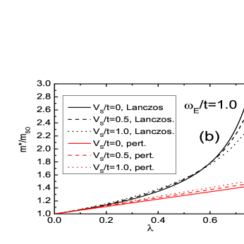
Figure 3: (color online)(a) Ground state energy difference $E_{GS}-E_{0}$ vs. $\lambda$ for $V_{S}/t=0,0.5,1.0$ and $\omega_{E}/t=1.0$. Exact numerical results are compared with those from weak coupling perturbation theory (labeled ”Pert.” in the figure) and from Lang-Firsov strong coupling theory. Agreement of both perturbative approaches with the exact numerical result is excellent. The MA result (not shown) is also in excellent agreement with the numerical results. (b)Effective mass $m^{\ast}/m_{SO}$ vs. $\lambda$. Numerical results are compared with that from weak coupling perturbation theory, and agreement is excellent for low values of $\lambda$. Both exact and perturbative approaches show an enhanced effective mass with increasing spin orbit coupling.

III.3 Numerical Results

In Fig. 3, we show the ground state energy and the effective mass correction as a function of electron-phonon coupling $\lambda$, with non-zero values of the spin orbit interaction, $V_{S}/t=0.5$ and $V_{S}/t=1.0$; these are compared with the results from the Holstein model with $V_{S}/t=0.$ Here the phonon frequency is set to be $\omega_{E}/t=1.0$, which is the typical value used in Ref.[covaci09, ], and for each value of $V_{S}$, the ground state energy is compared to the corresponding result for $\lambda=0$. The numerical results are compared with results from weak coupling perturbation theory and from Lang-Firsov strong coupling theory.

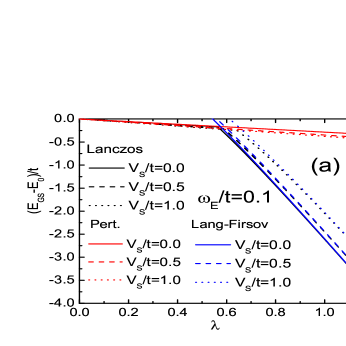
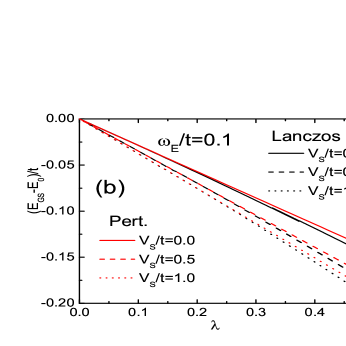
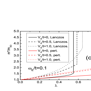
Figure 4: (color online) (a) Ground state energy $E_{GS}-E_{0}$ vs. $\lambda$ for $V_{S}/t=0,0.5,1.0$ and $\omega_{E}/t=0.1$. Exact numerical results are compared with those from weak coupling perturbation theory (labeled Pert. in the fig) and Lang-Firsov strong coupling theory. (b) Ground state energy $E_{GS}-E_{0}$ vs. $\lambda$ in the weak and intermediate coupling regime. (c) Effective mass $m^{\ast}/m_{SO}$ vs. $\lambda$. Numerical results are compared with those from weak coupling perturbation theory.

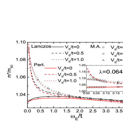
Figure 5: (color online) Effective mass $m^{\ast}/m_{SO}$ vs. $\omega_{E}/t$ for weak electron phonon coupling $\lambda=0.064$. In the inset the effective mass in the phonon frequency region near the adiabatic limit is shown. It is clear that the effective mass is enhanced as spin orbit interaction decreases near the adiabatic limit. This is in agreement with the result inferred from the electron density of states shown in Fig.2(a).

In Fig.3(a), the ground state energy crosses over smoothly (at around $\lambda\approx 0.8$) from the delocalized electron regime to the small polaron regime. Note that there is a slight dependence of the ground state energy on the spin orbit interaction. If we define $\Delta E=E_{GS}-E_{0},$ then $\Delta E(V_{S}/t=0.5)<\Delta E(V_{S}/t=0)<$ $\Delta E(V_{S}/t=1.0)\$in the delocalized electron regime, which is in agreement with the weak coupling perturbation theory, though this is barely visible in the figure. In the small polaron regime, the ground state energy is shifted up by the spin orbit interaction. This trend agrees with the results from Lang-Firsov strong coupling theory. For $V_{S}/t=0,$ the Lang-Firsov theory agrees very well with the numerical results, while as the spin orbit coupling $V_{S}$ increases, the Lang-Firsov theory becomes less accurate for the same electron phonon coupling (e.g. if we look at $\lambda=1.0$, for $V_{S}/t=1.0,$ the difference between Lang-Firsov theory and exact numerical results is larger than that for $V_{S}/t=0$). This is due to the fact that the bandwidth is increased by spin orbit interaction,covaci09 so the effective electron phonon coupling is decreased by spin orbit interaction. Better agreement with Lang-Firsov theory is achieved for larger values of $\lambda$. In Fig.3(b), the effective mass is enhanced by the spin orbit interaction in the delocalized electron regime, which is in agreement with the prediction from weak coupling perturbation theory. Here we have only shown results in the region $V_{S}/t=0\sim 1.0$; for larger values of $V_{S}/t$ the effective mass will be decreased by the spin orbit interaction in the delocalized regime.covaci09 In the small polaron regime, the effective mass will always be decreased by the spin orbit interaction.

In Fig.4, we show the same results as Fig. 3 for a much smaller phonon frequency $\omega_{E}/t=0.1$, which is closer to the adiabatic limit. In Fig.4(a), the ground state energy crosses over sharply (but still smoothly) from the delocalized electron regime to the small polaron regime. If we use $\lambda_{c}$ to describe the critical value for this sharp crossover, $\lambda_{c}$ will be enhanced significantly by the spin orbit interaction. For $V_{S}/t=0.0,\lambda_{c}\simeq 0.55,$while for $V_{S}/t=5.0,$ $\lambda_{c}\simeq 1.55$ from our numerical results. In Fig. 4(b), in the delocalized electron regime the ground state energy is decreased by the spin orbit interaction $\Delta E(V_{S}/t=1.0)<\Delta E(V_{S}/t=0.5)<$ $\Delta E(V_{S}/t=0.0)$, which is also in agreement with the weak coupling perturbation theory. For larger $V_{S}/t$ the ground state energy will be increasedcovaci09 in the delocalized electron regime. In the small polaron regime, the ground state energy will be increased by the spin orbit interaction, in agreement with the Lang-Firsov theory. In Fig.4(c), the effective mass enhancement for different spin orbit interaction $V_{S}/t$ is shown vs. electron phonon coupling strength, $\lambda$. For $V_{S}/t=0$ there is a rather sharp crossover from the delocalized electron regime to the small polaron regime.li10

Near the crossover point, the effective mass enhancement for the delocalized electron is around 1.4. For nonzero $V_{S}/t<1,$ near the crossover point, the effective mass enhancement is higher, but still within the same order of magnitute as $V_{S}/t=0$. This does not agree with the exact adiabatic limit $\omega_{E}/t\equiv 0$ of the Rashba-Holstein model which has been studied recently by Grimaldi,grimaldi10 based on a semiclassical method. He found that for nonzero spin orbit interaction $V_{S}$, the ground state will experience two phase transitions as the electron phonon coupling $\lambda$ is increased. The first transition is from a delocalized electron to a large polaron, while the second one is from a large polaron to a small polaron. In Fig.4(c), we observe only one sharp crossover from a delocalized electron to a small polaron. Our results did not exclude the possibilities that a large polaron regime will be found for $\omega_{E}/t<0.1$, although we find this possibility unlikely. A similar circumstance holds in the absence of a spin orbit coupling, where the adiabatic approximation gives rise to a single transition, while the quantum calculations results only in a crossover. Smaller values of $\omega_{E}$ can be explored, but quantum fluctuations become stronger for $\omega_{E}/t<0.1$ and the problem is numerically expensive for intermediate electron phonon coupling.

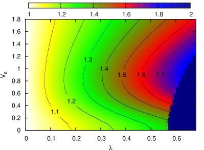
Figure 6: (color online) Effective mass $m^{\ast}/m_{SO}$ map as a function of spin orbit interaction $V_{S}/t$ and coupling constant $\lambda$ for $\omega_{E}/t=0.1$ obtained with the momentum average approximation.

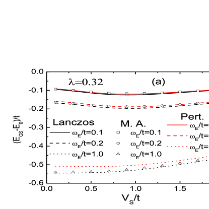
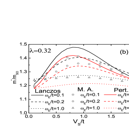
Figure 7: (color online)(a) Ground state energy $E_{GS}-E_{0}$ as a function of spin orbit interaction $V_{S}/t$ for $\omega_{E}/t=0.1,0.2,1.0$ at $\lambda=0.32$. (b) Effective mass $m^{\ast}/m_{SO}$ as a function of spin orbit interaction $V_{S}/t$ for the same parameters. Exact numerical results are compared with those from momentum averaging methods and weak coupling perturbation theory. The Momentum Average approximation does not do as well for low phonon frequencies.

To obtain some insight for the polaron effective mass near the adiabatic limit, we resort to weak coupling perturbation theory. In Fig.5 we observe an anomalous increase of the effective mass for small $\omega_{E}$ for nonzero $V_{S}$. However, the effective mass stops increasing as it reaches some finite number (around $1.2$ and $1.1$ for $V_{S}/t=0.5$ and $1.0$, respectively), so this does not indicate a breakdown of the perturbation theory. This result is confirmed by the MA results, as illustrated. This is also in agreement with results from the adiabatic limit. As shown in Fig. 2 of Ref.[grimaldi10, ], for $V_{S}/t=0.5$ and $1.0$ (his $\gamma/t=1.0$ and $2.0$), the electron is definitely in the delocalized electron regime for $\lambda=0.064$ ($\lambda=0.1$ in Ref.[grimaldi10, ]). Actually this anomalous increase of effective mass is caused by an increase in the value of the electron DOS at the bottom of the band, as shown in Fig. 2 and Eq. (9). Thus, for even smaller values of $V_{S}/t,$ the anomalous mass enhancement will increase further and perturbation theory will eventually break down. This is in agreement with the adiabatic limit results — as Fig. 2 of Ref.[grimaldi10, ] shows, for $V_{S}/t\simeq 0,$ the electron enters the large polaron regime for small $\lambda$. As mentioned earlier, our results are consistent with crossovers rather than transitions. This can be also seen in Fig. 6 where we plot for completeness a map of the effective mass as a function of $V_{s}/t$ and $\lambda$ obtained by using the MA approximation for $\omega_{E}/t=0.1$. The exact results, while different in the details, show the same qualitative trends.

In Fig. 7, we compare exact numerical results with both the momentum average methodcovaci09 and with weak coupling perturbation theory, for different values of $\omega_{E}.$ In Fig. 7(a), the ground state energy is shown as a function of $V_{S}/t$, while in Fig. 7(b), the effective mass is shown as a function of $V_{S}/t$. The MA method agrees well with the exact numerical results for $\omega_{E}/t=1.0$. For smaller values of $\omega_{E}$ ($\omega_{E}/t=0.1$ and $0.2$), the Momentum Average approximation becomes less accurate and agrees more closely with weak coupling perturbation theory. This is similar to what happens for the Holstein model. Reasons for this quantitative failure of MA in the adiabatic limit are explained in Ref. berciu06, .

IV Summary

In this paper we have studied the problem of a single electron coupled to oscillating ions, in the presence of a spin-orbit interaction. This problem has become relevant for a variety of spintronics applications. Many previous treatments have addressed this problem with a finite density of electrons, and have therefore necessarily required approximate theoretical methods for solution. The limit of only one electron, previously solved with weak coupling perturbation methods and with the momentum average approximation, is amenable to exact solution as described here, and serves as a benchmark to which other, approximate solutions must converge. Moreover, in many dilute semiconductor applications, the single electron result may be the relevant regime required for understanding of the problem.

The exact method of solution utilizes the Trugman method of solution,bonca99 through Lanczos diagonalization. The procedure for this is now well documented, and converges very quickly over a very wide parameter regime. The momentum average approximationcovaci09 also works very well over the entire parameter regime; there is a breakdown for very low phonon frequencies. In this regime the adiabatic approximationgrimaldi10 provides a good qualitative picture. Weak coupling perturbation theorycappelluti07 tends to be fairly accurate only for very small coupling strengths. Finally, strong coupling perturbation theorymarsiglio95 is very accurate in the small polaron regime.

In weak coupling the presence of spin orbit coupling increases the effective mass of the electron coupled to Einstein phonons.cappelluti07 The effective mass is small to begin with, so in this regime the impact of spin orbit coupling is fairly minor. As the electron phonon coupling increases, and one enters the small polaron regime, the presence of spin orbit coupling has the opposite effect, as first noted with the momentum average approximation.covaci09 Since in this regime the effective masses can be quite large, spin orbit coupling can have a profound effect on the characteristics of the electron.

Appendix A Density of states at the bottom of the band

Expanding $\varepsilon_{k,-}$ around the minimum energy $E_{0}$, by defining $k_{x}^{\prime}=k_{x}\pm\arctan(\frac{V_{S}}{\sqrt{2}t}),k_{y}^{\prime}=k_{y}\pm\arctan(\frac{V_{S}}{\sqrt{2}t}),$ we have

$$\varepsilon_{k,-}-E_{0}=\frac{0.5t}{\sqrt{1+V_{S}^{2}/(2t^{2})}}[(1+V_{S}^{2}/t^{2})(k_{x}^{\prime 2}+k_{y}^{\prime 2})\pm 2k_{x}^{\prime}k_{y}^{\prime}]$$ (21)

To calculate the density of states at the bottom of the band, from the definition, we have

$$D_{-}(E_{0}+E_{1})=\frac{1}{4\pi^{2}}\int_{-\pi}^{\pi}dk_{x}\int_{-\pi}^{\pi}dk_{y}\delta(E_{0}+E_{1}-\varepsilon_{k,-}),$$ (22)

where $E_{1}$ is a small amount of energy above the bottom of the band, $E_{0}$. Around the four energy minimum points there are four small regions which will contribute to this integral. We choose one of them (and then times our results by a factor of 4) and use the definitions of $k^{\prime}$ above instead of $k,$ introduce a small cutoff $k_{c}$ which is the radius of a small circle around $k_{\min},$ thus the integral reads

$$D_{-}(E_{0}+E_{1})=4\times\frac{1}{4\pi^{2}}\int_{0}^{k_{c}}k^{\prime}dk^{\prime}\int_{-\pi}^{\pi}d\theta$$ (23)

$$\times\delta(E_{1}-\frac{0.5t}{\sqrt{1+V_{S}^{2}/(2t^{2})}}[(1+V_{S}^{2}/t^{2})+\sin 2\theta]k^{\prime 2})$$

$$= \frac{\sqrt{1+V_{S}^{2}/(2t^{2})}}{\pi^{2}t}\int_{-\pi}^{\pi}d\theta\frac{1}{[(1+V_{S}^{2}/t^{2})+\sin 2\theta]}$$

$$= {\sqrt{2}\over\pi}{1\over V_{S}}.$$

The derivation of the effective mass in the weak coupling approximation (Eq. (20)) proceeds similarly. We begin with Eq. (18) in the text for the self energy. For very small phonon frequency we need only focus on the lower Rashba band, $s=-1$. Furthermore, the non-interacting electron energy can be expanded about a minimum, as in Eq. (21). Noting that there are four equal contributions coming from the four degenerate minima, we obtain

$$\Sigma_{\rm weak}(\omega+i\delta)=-4\frac{\pi\lambda t\omega_{E}}{(2\pi)^{2}}\int dk_{x}^{\prime}\int dk_{y}^{\prime}$$

$$\frac{1}{a^{2}+\frac{t}{2\sqrt{1+{V_{S}^{2}\over 2t^{2}}}}\biggl{[}(1+(V_{S}/t)^{2})(k_{x}^{\prime 2}+k_{y}^{\prime 2})+2k_{x}^{\prime}k_{y}^{\prime}\biggr{]}}$$ (24)

where $a^{2}=E_{0}+\omega_{E}-\omega$, and the integration is understood to be around a small disk located at one of the energy minima. Transforming to polar coordinates allows both the radial and angular integral to be done analytically; for the radial integral we keep only the dominant portion for small $\omega_{E}$, and, after differentiation, we readily obtain the result quoted in the text (Eq. (20)).

Appendix B Strong coupling limit

To investigate the strong coupling limit using second order perturbation, we need to evaluate Eq. (15), repeated here for convenience:

$$E_{k-}^{(2)}=\sum_{n_{TOT}\neq 0,n1,n2,...=0,1,...\infty}\ \sum_{\ell=1\atop\sigma}^{N}$$

$$\frac{\left|\langle n_{1},n_{2},...n_{N}|_{ph}\otimes\langle c_{\ell\sigma}|_{el}\overline{T}|\Psi_{k,-}\rangle_{el}\otimes|0\rangle_{ph}\right|^{2}}{-n_{TOT}\omega_{E}}$$

$$=\frac{-t^{2}e^{-2g^{2}}}{\omega_{E}}\sum_{{n1,n2..=0}\atop{n_{\rm TOT}\neq 0}}^{\infty}\ \sum_{\ell=1}^{N}\frac{|A_{\uparrow}|^{2}+|A_{\downarrow}|^{2}}{n_{\rm TOT}},$$ (25)

where $A_{\sigma}$ is given a series of matrix elements (distinct for $\sigma=\uparrow$ and $\downarrow$). These turn out to give equal contributions, so we illustrate in some detail the result for $A_{\uparrow}$ only. After some algebra, we obtain

$$|A_{\uparrow}|^{2}=|u_{\ell}(-g)|^{2}\ |\sum_{\delta=\pm x,\pm y}c_{\delta}u_{\ell+\delta}(g)|^{2},$$ (26)

where

$$u_{\ell}(\pm g)\equiv\langle n_{\ell}|e^{\pm ga_{\ell}^{\dagger}}|0\rangle=\frac{(\pm g)^{n_{\ell}}}{\sqrt{n_{\ell}!}}$$ (27)

and

$$c_{+x} = e^{+ik_{x}a}\bigl{(}1+\frac{V_{S}}{t}e^{i\phi_{k}}\bigr{)}$$

$$c_{-x} = e^{-ik_{x}a}\bigl{(}1-\frac{V_{S}}{t}e^{i\phi_{k}}\bigr{)}$$

$$c_{+y} = e^{+ik_{y}a}\bigl{(}1-i\frac{V_{S}}{t}e^{i\phi_{k}}\bigr{)}$$

$$c_{-y} = e^{-ik_{y}a}\bigl{(}1+i\frac{V_{S}}{t}e^{i\phi_{k}}\bigr{)},$$ (28)

and

$$e^{i\phi_{k}}\equiv\frac{\sin{(k_{y}a)}-i\sin{(k_{x}a)}}{\sqrt{\sin^{2}{(k_{x}a)}+\sin^{2}{(k_{y}a)}}}.$$ (29)

For each of the $u_{\ell}(\pm g)$ in Eq. (26) it is to be understood that $n_{\ell}\neq 0$, but all other $n_{\ell{{}^{\prime}}}=0$ for $\ell^{\prime}\neq\ell$. Hence, in the 16 terms in Eq. (26), 12 will have all phonon numbers equal to zero (other than $n_{\ell}$); the other 4 will have both $n_{\ell}$ and $n_{\ell+x}$ (or $n_{\ell}$ and $n_{\ell-x}$, etc.) not equal to zero in general. As already mentioned, the contribution from $|A_{\downarrow}|^{2}$ is identical to that from $|A_{\uparrow}|^{2}$, so this merely gives us a factor of $2$ in Eq. (25). Moreover, translational invariance makes the contribution from each site identical, so the sum over sites is trivially performed. This equation then becomes

$$E_{k-}^{(2)}=-\frac{4t^{2}e^{-2g^{2}}}{\omega_{E}}\{f(g^{2})\bigl{(}\frac{\epsilon_{k-}}{2t}\bigr{)}^{2}+\bigl{[}f(2g^{2})-f(g^{2})\bigr{]}\bigl{[}1+(\frac{V_{S}}{t})^{2}\bigr{]}\},$$ (30)

where

$$f(x) \equiv \sum\limits_{n=1}^{\infty}\frac{1}{n}\frac{x^{n}}{n!}=Ei(x)-\gamma-\ln{x}$$ (31)

$$\approx e^{x}/x\bigl{[}1+1/x+2/x^{2}+...\bigr{]},$$

and $Ei(x)$ is the exponential integral and $\gamma\approx 0.5772$ is Euler’s constant. Eq. (30) leads directly to Eq. (16) in the text.

^∗ present address: Dept. of Oncology, University of Alberta, Edmonton, AB, Canada T6G 1Z2

References

- (1) J.J. Sakurai, Advanced Quantum Mechanics (Addison-Wesley, Don Mills, 1967).
- (2) R. Winkler, Spin-Orbit Coupling Effects in Two-Dimensional Electron and Hole Systems (Springer, Berlin, 2003).
- (3) S. A. Wolf, D. D. Awschalom, R. A. Buhrman, J. M. Daughton, S. von Moln‡r, M. L. Roukes, A. Y. Chtchelkanova and D. M. Treger, Science 294, 1488, (2001).
- (4) E.I. Rashba, Sov. Phys. Solid State 2, 1109 (1960).
- (5) E. Rotenberg, J. W. Chung, and S. D. Kevan, Phys. Rev. Lett. 82, 4066, (1999).
- (6) D. Pacilé, C.R. Ast, M. Papagno, C. Da Silva, L. Moreschini, M. Falub, A. P. Seitsonen, and M. Grioni, Phys. Rev. B 73, 245429 (2006).
- (7) C. R. Ast, G. Wittich, P. Wahl, R. Vogelgesang, D. Pacilé, M. C. Falub, L. Moreschini, M. Papagno, M. Grioni, and K. Kern, Phys. Rev. B 75, 201401(R), (2007).
- (8) C. R. Ast, J. Henk, A. Ernst, L. Moreschini, M. C. Falub, D. Pacilé, P. Bruno, K. Kern, and M. Grioni, Phys. Rev. Lett. 98, 186807, (2007).
- (9) E. Cappelluti, C. Grimaldi and F. Marsiglio, Phys. Rev. Lett 98, 167002 (2007); Phys. Rev. B76, 085334 (2007). See also, C. Grimaldi, E. Cappelluti, and F. Marsiglio, Phys. Rev. Lett. 97, 066601 (2006); Phys. Rev. B73, 081303(R) (2006).
- (10) T. Holstein, Ann. Phys. (New York) 8, 325 (1959).
- (11) L. Covaci and M. Berciu, Phys. Rev. Lett 102, 186403 (2009).
- (12) M. Berciu, Phys. Rev. Lett 97, 036402 (2006); M. Berciu and G. L. Goodvin, Phys. Rev. B 76, 165109 (2007).
- (13) S.A. Trugman, in Applications of Statistical and Field Theory Methods to Condensed Matter, edited by D. Baeriswyl, A.R. Bishop, and J. Carmelo (Plenum Press, New York, 1990).
- (14) J. Bonča, S.A. Trugman, and I. Batistíc, Phys. Rev. B60,1633 (1999).
- (15) Zhou Li, D. Baillie, C. Blois, and F. Marsiglio, Phys. Rev. B81, 115114, (2010).
- (16) A. Alvermann, H. Fehske, and S. Trugman, Phys. Rev. B 81, 165113 (2010).
- (17) I.G. Lang and Yu. A. Firsov, Sov. Phys. JETP16, 1301 (1963); Sov. Phys. Solid State 5 2049 (1964).
- (18) F. Marsiglio, Physica C244 21, (1995).
- (19) C. Grimaldi, Phys. Rev. B 81, 075306 (2010).
- (20) A. Lagendijk and H. De Raedt, Phys. Letts. A108, 91 (1985).
- (21) V.V. Kabanov and O.Yu Mashtakov, Phys. Rev. B47, 6060 (1993).