Effects of non-resonant interaction in ensembles of phase oscillators

Abstract

We consider general properties of groups of interacting oscillators, for which the natural frequencies are not in resonance. Such groups interact via non-oscillating collective variables like the amplitudes of the order parameters defined for each group. We treat the phase dynamics of the groups using the Ott-Antonsen ansatz and reduce it to a system of coupled equations for the order parameters. We describe different regimes of co-synchrony in the groups. For a large number of groups, heteroclinic cycles, corresponding to a sequental synchronous activity of groups, and chaotic states, where the order parameters oscillate irregularly, are possible.

I Introduction

Models of coupled limit cycle oscillators are widely used to describe self-synchronization phenomena in various branches of science. The applications include physical systems like Josephson junctions Wiesenfeld and Swift (1995), lasers Glova (2003), and electrochemical oscillators Kiss et al. (2002), but similar models are also used for neuronal ensembles Golomb et al. (2001), the dynamics of pedestrians on bridges Strogatz et al. (2005); Eckhardt et al. (2007), applauding persons Néda et al. (2000), etc.

In many cases a model of a fully connected (globally coupled) network is appropriate, it means that the oscillator population is treated in the mean field approximation. Ensembles of weakly interacting self-sustained oscillators are successfully handled in the framework of phase approximation Kuramoto (1975, 1984); Daido (1992, 1993, 1996). Most popular are the Kuramoto model of sine-coupled phase oscillators, and its extension, the Kuramoto-Sakaguchi model Sakaguchi and Kuramoto (1986). This model describes self-synchronization and appearance of a collective mode (mean field) in an ensemble of generally non-identical elements as a nonequilibrium phase transition. The basic assumptions behind the Kuramoto model are that of weak coupling and of closeness of frequencies of oscillators, the latter results in the presence of resonant terms in the coupling function only. References to detailed aspects of the Kuramoto model can be found in Pikovsky et al. (2001); Acebron et al. (2005); Strogatz (2000).

In many cases the ensembles of oscillators are not uniform and can be considered as consisting of several subensembles (e.g., in brain different groups of neurons can have different characteristic rhythms). If one still assumes that the frequencies of these subgroups are close (compared to the coupling), then a model of several interacting subpopulations Tukhlina and Rosenblum (2008); Popovych and Tass (2010) or of an ensemble having a bimodal (or a multi-modal) distribution of frequencies Bonilla et al. (1992); Crawford (1994); Bonilla et al. (1998); Bonilla (2000); Montbrió et al. (2006); Martens et al. (2009); Pazó and Montbrió (2009) is adopted. Similarly, one can also model two ensembles, one of which consists of active and another of passive elements, which are coupled resonantly due to closeness of their frequencies Daido and Nakanishi (2004); Pazó and Montbrió (2006).

In this paper we study a novel situation of non-resonantly coupled oscillator ensembles. We assume that there are several groups of oscillators, the frequencies in each group are close to each other, but are strongly (compared to the coupling strength) different between the groups. In this situation the coupling within the group is resonant, like in usual Kuramoto-type models, but the coupling between the groups can be only non-resonant . It means that the coupling can be via non-oscillating, slow variables only, i.e. via the amplitudes of the mean fields. In the context of a single Kuramoto model such a dependence on the amplitude of the mean field corresponds to a nonlinearity of coupling, recently studied in Rosenblum and Pikovsky (2007); Pikovsky and Rosenblum (2009); Filatrella et al. (2007); Giannuzzi et al. (2007). Nonlinearity in this context means that the effect of the collective mode on an individual unit depends on the amplitude of this mode, so that, e.g., the interaction of the field and of a unit can be attractive for a weak field and repulsive for a strong one. Mathematically, this is represented by the dependence of the parameters of the Kuramoto-Sakaguchi model (the coupling strength, the effective frequency spreading, and the phase shift) on the mean field amplitude. Here we generalize this approach to several ensembles, so that the parameters of the Kuramoto-Sakaguchi model describing each subgroup depend on the mean field amplitudes of other subgroups (e.g., resonant interactions within a group of oscillators can be attractive or repulsive dependent on the amplitude of the order parameter of another group).

In Section II we introduce the basic model of non-resonantly interacting ensembles. We also formulate the equations for the mean fields of the ensembles following the Ott-Antonsen theory Ott and Antonsen (2008, 2009). The simplest situation of two interacting ensembles is studied in Section III. In Section IV we describe three and several interacting ensembles, focusing on nontrivial regimes of sequential synchronous activity following a heteroclinic cycle, and on chaotic dynamics.

II Basic model of non-resonantly interacting oscillator ensembles

II.1 Kuramoto-Sakaguchi model and Ott-Antonsen equations for its dynamics

A popular model describing resonant interactions in an ensemble of oscillators having close frequencies is due to Kuramoto and Sakaguchi Sakaguchi and Kuramoto (1986)

$$\dot{\phi}_{k}=\omega_{k}+\text{Im}(KZe^{-i\phi_{k}}),\qquad Z=\frac{1}{N}\sum e^{i\phi_{k}},\qquad k=1,\ldots,N.$$ (1)

Here $\phi_{k}$ is oscillator’s phase, $Z$ is the complex order parameter (mean field) that also serves as a measure for synchrony in the ensemble, $\omega_{k}$ are natural frequencies of oscillators, and $K=2a+2ib$ is a complex coupling constant. Recently, Ott and Antonsen Ott and Antonsen (2008, 2009) have demonstrated that in the thermodynamic limit $N\to\infty$, and asymptotically for large times the evolution of the order parameter $Z$ in the case of a Lorentzian distribution of natural frequencies $g(\omega)=\Delta[\pi(\omega-\omega_{0})^{2}+\Delta^{2}]^{-1}$ around the central frequency $\omega_{0}$ is governed by a simple ordinary differential equation

$$\dot{Z}=(i\omega_{0}-\Delta)Z+\frac{1}{2}(K-K^{*}|Z|^{2})Z.$$ (2)

Written for the amplitude and the phase of the order parameter defined according to $Z=\rho e^{i\Phi}$, the Ott-Antonsen equations

$$\dot{\rho} =-\Delta\rho+a(1-\rho^{2})\rho\;,$$ (3)

$$\dot{\Phi} =\omega_{0}+2b\rho^{2}\;,$$ (4)

are easy to study: Eq. (3) defines the stationary amplitude of the mean field (which is non-zero above the synchronization threshold $a_{c}=\Delta$), while Eq. (4) yields the frequency of the mean field.

II.2 Non-resonantly interacting ensembles

We consider several ensembles of oscillators, each characterized by its own parameters $\omega_{0},\Delta,a,b$. The main assumption is that the central frequencies $\omega_{0}$ of different populations are not close to each other, and also high-order resonances between them are not present. Such a situation appears typical for neural ensembles, where different areas of brain demonstrate oscillations in a very broad range of frequencies, from alpha to gamma rhythms. Because there is no resonant interaction between the oscillators in different ensembles, they can interact only non-resonantly, via the absolute values of the mean fields. Assuming that only Kuramoto order parameters (1) (but not higher-order Daido order parameters $Z_{m}=\langle e^{im\phi}\rangle$) enter the coupling, a general non-resonant interaction between populations can be described by the dependencies of the parameters $\omega_{0},\Delta,a,b$ on the amplitudes of the mean fields $\rho_{l}$, where index $l$ counts the subpopulations. Moreover, one can see from (3,4) that the equation for the amplitude is independent on the phase, therefore we can restrict our attention to the amplitude dynamics (3). Furthermore, we assume the coupling to be week, so only the leading order corrections $\sim\rho^{2}$ are included. All this leads to the following general model for interacting populations

$$\dot{\rho}_{l}=(-\Delta_{l}-\Gamma_{lm}\rho_{m}^{2})\rho_{l}+(a_{l}+A_{lm}\rho_{m}^{2})(1-\rho_{l}^{2})\rho_{l},\qquad l=1,\dots,L$$ (5)

with coupling constants $\Gamma_{lm},A_{lm}$. Note that because the widths of the frequencies distribution cannot be negative, coefficients $\Gamma_{lm}$ must satisfy $\Delta_{l}+\Gamma_{lm}\geq 0$. Below we assume that there is no nonlinearity inside ensembles $\Gamma_{ll}=A_{ll}=0$.

In this paper we will not investigate model (5) in its full generality, as it would require a rather tedious analysis. Instead, we will consider two simpler models, which describe particular types of interaction, but nevertheless allow us to demonstrate interesting dynamical patterns. In model A we assume that only frequencies are influenced by the coupling, i.e. $A_{lm}=0$. This leads to a system

$$\dot{\rho}_{l}=(a_{l}-\Delta_{l}-\Gamma_{lm}\rho_{m}^{2}-a_{l}\rho_{l}^{2})\rho_{l}$$ (6)

Another model B takes into account the interaction via coupling constants only (i.e. $\Gamma_{lm}=0$); additionally we will assume here that the distributions of frequencies in all interacting ensembles are narrow $\Delta_{l}\to 0$. In the limit of identical oscillators we obtain from (5)

$$\dot{\rho}_{l}=(a_{l}+A_{lm}\rho_{m}^{2})(1-\rho_{l}^{2})\rho_{l}$$ (7)

Here we note that the Ott-Antonsen equations for the ensemble of identical oscillators describe not a general case, but a particular solution, while a general description delivers the Watanabe-Strogatz theory Watanabe and Strogatz (1994); Pikovsky and Rosenblum (2008). Thus the dynamics of model B should be considered as a special singular limit $\Delta\to 0$.

Below, in sections III and IV we describe the dynamics of these two models, for the cases of two, and three and more interacting ensembles, respectively.

III Two interacting ensembles

Let us first rewrite models (6,7) for the simplest case of only two interacting ensembles. Additionally, for model A we assume $a_{l}=1$ (equivalently, one could renormalize the amplitudes of order parameters $\rho_{1,2}$ to get rid of these coefficients). Thus the model A reads

$$\dot{\rho}_{1} =\rho_{1}(\delta_{1}-d_{12}\rho_{2}^{2}-\rho_{1}^{2})\;,$$ (8)

$$\dot{\rho}_{2} =\rho_{2}(\delta_{2}-d_{21}\rho_{1}^{2}-\rho_{2}^{2})\;.$$

For model B a normalization of amplitudes is not possible, and it reads

$$\dot{\rho}_{1} =\varepsilon_{1}\rho_{1}(1-D_{12}\rho_{2}^{2})(1-\rho_{1}^{2})\;,$$ (9)

$$\dot{\rho}_{2} =\varepsilon_{2}\rho_{1}(1-D_{21}\rho_{1}^{2})(1-\rho_{2}^{2})\;.$$

Generally, parameters $\delta_{1,2}=1-\Delta_{1,2},\;d_{ik}=\Gamma_{ik},\;\varepsilon_{1,2}=a_{1,2},\;D_{ik}=-A_{ik}/a_{i}$ can have different signs.

As the first property of both models we mention that the dynamics is restricted to the domain $0\leq\rho_{1,2}\leq 1$. Formally, this follows directly from (5), physically this corresponds to the admissible range of values of the order parameter. Furthermore, for model A (8) we can apply the Bendixon-Dulac criterion

$$\frac{\partial}{\partial\rho_{1}}\left(\frac{1}{\rho_{1}\rho_{2}}\dot{\rho}_{1}\right)+\frac{\partial}{\partial\rho_{2}}\left(\frac{1}{\rho_{1}\rho_{2}}\dot{\rho}_{2}\right)=-2\frac{\rho_{1}^{2}+\rho_{2}^{2}}{\rho_{1}\rho_{2}}<0$$

from which it follows that it cannot possess periodic orbits.

Remarkably, model B (9) can be written as a Hamiltonian one. With an ansatz

$$\exp y_{1,2}=\rho_{1,2}^{2}(1-\rho_{1,2}^{2})^{-1}$$ (10)

it can be represented in a Hamiltonian form

$$\begin{gathered}\dot{y}_{1}=\frac{\partial H(y_{1},y_{2})}{\partial y_{2}},\qquad\dot{y}_{2}=-\frac{\partial H(y_{1},y_{2})}{\partial y_{1}},\\ \qquad H=2\varepsilon_{1}y_{2}-2\varepsilon_{2}y_{1}-2\varepsilon_{1}D_{12}\ln(1+e^{y_{2}})+2\varepsilon_{2}D_{21}\ln(1+e^{y_{1}})\;.\end{gathered}$$ (11)

Thus model B may demonstrate a family of periodic orbits if the levels of the Hamiltonian are closed curves. We stress that the Hamiltonian structure of the model does not exclude existence of stable equilibria at $\rho=0,1$ because the transformation (10) is singular at these states; in the Hamiltonian formulation (11) these stable equilibria correspond to trajectories moving toward $\mp\infty$.

The dynamics of both models is mainly determined by the existence and stability of equilibria. For model A (8) possible equilibria are the trivial one $S_{1}(0,0)$, two states where one of the order parameters vanish $S_{2}(\delta_{1}^{1/2},0)$ and $S_{3}(0,\delta_{2}^{1/2})$, and a state where both order parameters are non-zero $S_{4}((\delta_{1}-d_{12}\delta_{1})(1-d_{12}d_{21})^{-1},(\delta_{2}-d_{21}\delta_{1})(1-d_{12}d_{21})^{-1})$. Similarly, model B (9) always has equilibria $M_{1}(0,0)$, $M_{2}(1,0)$, $M_{3}(0,1)$ and $M_{4}(1,1)$, and additionally a nontrivial state $M_{5}(D_{21}^{-1/2},D_{12}^{-1/2})$ existing if $D_{12},D_{21}>1$.

We illustrate possible types of dynamics (up to symmetry $1\leftrightarrow 2$) in models A,B in Figs. 1,2. Here it is worth mentioning, that model (8) is structurally of the same type as typical models of interacting populations in mathematical ecology Murray (2002). Model B (9) resembles them as well, but has a distinctive property that fully synchronized cluster $\rho=1$ is invariant. Referring for the details to Appendix A, we describe briefly possible regimes in these models.

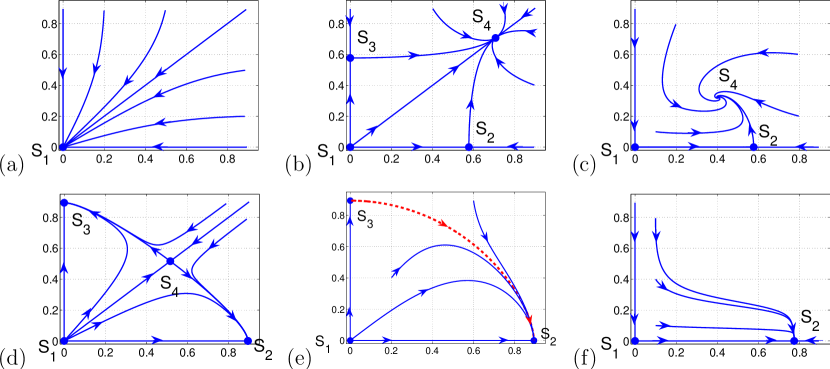
Figure 1: (Color online) Six different patterns of the dynamics of system (8). (a) Global stability of a trivial state (for $\delta_{1,2}<0$). (b,c) Global stability of $S_{4}$ when both populations are partially synchronous (conditions for this are (14) for (b) or (15) for (c)). (d) Competition between clusters if the coupling is strongly suppressive (18)); here we have bistablity of states $S_{2,3}$ describing synchronous activity of one cluster and asynchronous of another one. (e) Asymmetric interaction between clusters arises under condition (20); here always a heteroclinic trajectory from saddle point $S_{3}$ to stable node $S_{2}$ exists (red dashed line). (f) Global stability of $S_{2}$ under condition (20).

1. Global stability of trivial equilibrium point $S_{1}(0,0),\ M_{1}(0,0)$ (Fig.1a, Fig.2a,b) means that a fully asynchronous state is stable in both ensembles.

2. Stability of a nontrivial state off coordinate axes $S_{4}$ and $M_{4}$ (Fig.1b,c, Fig.2c,d). Here both ensembles are synchronized (in model A not completely because of a distribution of frequencies, in model B completely because we assume identical oscillators in ensembles).

3. Competition between ensembles (Fig.1d,2e): Only one ensemble synchronizes while the other one desynchronizes. Which ensemble is synchronous depends on initial conditions.

4. Suppression: One ensemble always “wins” and is synchronous while the other one desynchronizes (steady states $S_{2}$,$M_{2}$ are global attractors, of course also stability of “symmetric” states $S_{3},M_{3}$ is possible)(Fig.1e,f,2f,g,h).

5. The case of bistability of the trivial and the fully synchronous states of both ensembles (Fig.2i) is possible in the model B only.

6. Periodic behavior (Fig.2j) is possible only in ensemble B, it corresponds to an interaction of populations of “predator-pray” type. Because of the system is Hamiltonian, the oscillations are conservative like in the Lottka-Volterra system.

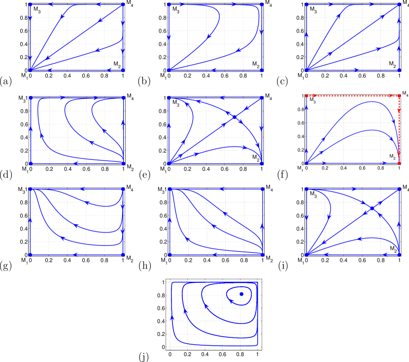
Figure 2: (Color online) Ten different dynamical regimes in system (9). (a,b): Global stability of the trivial state, arises at conditions (13). Case (a): $D_{12}<1$, case (b): $D_{12}>1$. (c,d): Global stability of $M_{4}(1,1)$ when both clusters are in the synchronized state, under condition of a weak suppressive coupling (16) for (c) or at (17) for (d). (e): Competition between clusters, arises at strong suppressive coupling (19). Here we have bistablity of steady states $M_{2,3}$; each of these points corresponds to synchronous activity of one cluster and asynchronous of another one. (f): Asymmetric interaction between clusters at asymmetric coupling (23). Here always a sequence of heteroclinic trajectories $M_{3}\to M_{4}\to M_{2}$ (red dashed lines) is present. (g,h): The situation of global stability of fixed point $M_{3}$ while conditions (22) are satisfied (case (g): $D_{21}>1$, case (h): $D_{21}<1$). (i): Bistablity of fully asynchronous and fully synchronous states, arises if (24) is valid. In this case stable manifolds of the saddle point $M_{5}$ divide basins of attraction of stable points $M_{1}$, $M_{4}$. (j): The case of periodic behavior, arises at conditions (25).

While in our analysis we studied models (8,9) describing dynamics of the order parameters in the Ott-Antonsen ansatz, all the regimes described above can be observed when one simulates original equations of the ensembles of phase oscillators (1), at sufficiently large number of units $N$. In Fig. 3 we illustrate two nontrivial regimes of two subpopulations of phase oscillators at $N=10^{3}$. Figure 3(a) shows the dynamics of mean fields in the case of a competition between two subpopulations that interact via frequency mismatch modulation, see Fig. 1(d). Figure 3(b) illustrates a periodic behavior of two subpopulations like in Fig. 2(j).

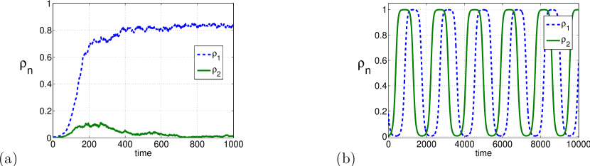
Figure 3: (Color online) Modeling of ensemble consisting of two subpopulations of $N=10^{3}$ phase oscillators. (a) Subpopulations interact via modulation of effective frequency mismatch (8). Case of competition between subpopulations for parameter values $\delta_{1,2}=10$, $d_{12}=d_{21}=12$. (b) Subpopulations interact via coupling modulations (9). A periodic regime is presented at parameter values $\varepsilon_{1}=-1$, $\varepsilon_{2}=1$, $D_{12}=D_{21}=2$. To avoid a spurious clustering and to ensure validity of Ott-Antonsen description, a small mismatch was added: $\omega_{n}$ were randomly distributed in the range $[-0.025,+0.025]$.

IV Three and more interacting ensembles

In this section we generalize the results of Section III to many interacting ensembles. We do not aim here at the full generality, but rather present interesting regimes based on the elementary dynamics depicted in Figs. 1,2. According to the consideration above, we restrict our attention to two basic models A (6) and B (7). Generally, model B cannot be rewritten in a Hamiltonian form, but by applying transformation (10) one can easily see that this system has a Liouvillian property – the phase volume is conserved.

IV.1 Symmetric case: cosynchrony and competition

Here we describe mostly simple regimes that are observed in a symmetric case where parameters of all ensembles and their interaction are equal. This corresponds to equal values $a_{l}=a,\Delta_{l}=\Delta,\Gamma_{lm}=\Gamma$ in (6) and $a_{l}=a,A_{lm}=A$ in (7). In model A, the only nontrivial regimes are those where asynchronous states are unstable $\Delta<a$. Then one observes either a coexistence of synchrony like in Fig. 1b (for $\Gamma<a$) or a competition like in Fig. 1d (for $\Gamma>a$). In the latter case only one ensemble is synchronous, while other desynchronize. Similar regimes can be observed in model B for $a>0$, $A<-a$. Additionally, in model B a coexistence of full synchrony in all ensembles and a full asynchrony, like in Fig. 2i can be observed for $a<0$, $A>-\frac{a}{L-1}$. We illustrate the regimes of competition in Fig. 4 for the case of three interacting populations.

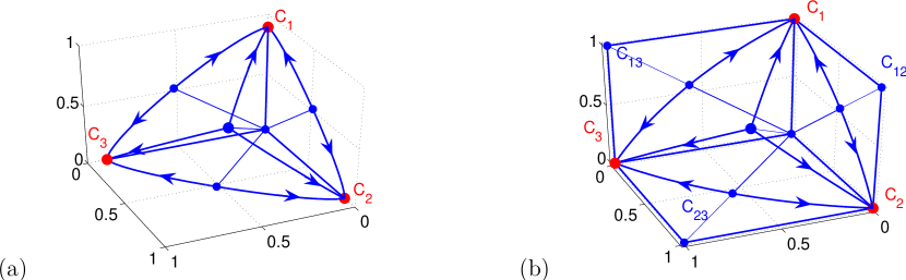
Figure 4: (Color online) Multistability of steady states $C_{n}$ corresponding to synchronous state of only one cluster for (a) system (6) ($\Delta>a$, $\Gamma>a$) and (b) system (7) ($a>0$, $A<-a$).

IV.2 Heteroclinic synchrony cycle

Here we discuss a multidimensional generalization of the interactions where in a pair of ensembles one group always synchronizes while another one is asynchronous (see Figs. 1(e),2(f)). In the examples presented in these graphs, both ensembles would self-synchronize separately, but due to interaction synchrony in ensemble 2 disappears while ensemble 1 remains synchronous. One can say that in synchrony competition between the first and the second ensembles, the first ensemble wins. Suppose now, that a third self-synchronizing ensemble is added, which wins in the competition with the first one but looses in the competition to the second one. Then a cycle $2\to 1\to 3\to 2\to 1\to 3\ldots$ will be observed. Moreover, because in the dynamics Figs. 1(e),2(f) the transition $2\to 1$ follows the heteroclinic orbit connecting steady states $S_{3}$ and $S_{2}$, the cycle in the system of three ensembles will be a heteroclinic one, with asymptotically infinite period. Such a cycle has been studied in different contexts Busse and Clever (1979); Clune and Knobloch (1994); Guckenheimer and Holmes (1988). For a review of robust heteroclinic cycles see Krupa (1997); V. Afraimovich, P. Ashwin, and V. Kirk, Editors (2010) (sometimes one uses a term “winnerless competition” to describe such a dynamics Rabinovich et al. (2001); Afraimovitch et al. (2008)).

We demonstrate the heteroclinic synchrony cycle for three interacting ensembles in Fig. 5. One can see that synchronous states of ensembles appear for longer and longer time intervals. It is interesting to note that heteroclinic cycles have been observed in ensembles of identical coupled oscillators Ashwin and Swift (1992); Hansel et al. (1993); Kori and Kuramoto (2001); Kori (2003); Ashwin and Borresen (2004, 2005). There the nontrivial dynamics is in the switchings of full synchrony between different clusters. In this respect the heteroclinic cycle in the model B resembles such a regime. On the other hand, the heteroclinic cycle in model A is different: here the natural frequencies of oscillators are different and the states of synchrony are not complete, so the identical clusters never appear.

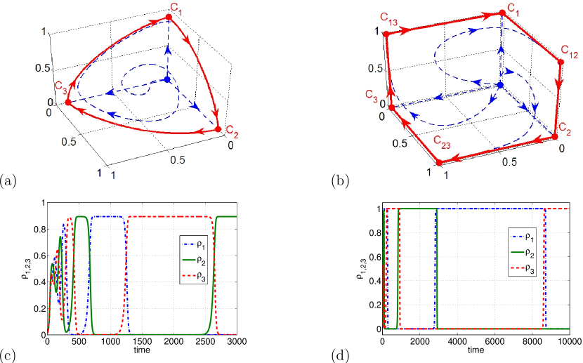
Figure 5: (Color online) Stable heteroclinic cycles caused by asymmetric interactions between clusters in system (6) (a,c) and in system (7) (b,d). Parameters: (a,c) $a_{l}-\delta_{l}>0$, $\Gamma_{12}>\frac{a_{2}(a_{1}-\delta_{1})}{a_{2}-\delta_{2}}$, $\Gamma_{31}>\frac{a_{1}(a_{3}-\delta_{3})}{a_{1}-\delta_{1}}$, $\Gamma_{23}>\frac{a_{3}(a_{2}-\delta_{2})}{a_{3}-\delta_{3}}$, $\Gamma_{21}<\frac{a_{1}(s_{2}-\delta_{2})}{a_{1}-\delta_{1}}$, $\Gamma_{13}<\frac{a_{3}(a_{1}-\delta_{1})}{a_{3}-\delta_{3}}$, $\Gamma_{32}<\frac{a_{2}(a_{3}-\delta_{3})}{a_{2}-\delta_{2}}$, (d) $a_{l}>0$, $A_{12}<-a_{1},\ A_{31}<-a_{3},\ A_{23}<-a_{2}$, $A_{21}>-a_{2},\ A_{13}>-a_{1},\ A_{32}>-a_{3}$. Panels (a,b) show the phase space portraits while time series are presented in panels (c,d).

Finite size effects are nontrivial for the heteroclinic cycles described. Indeed, it is known that while in the thermodynamic limit deterministic equations for the order parameters can be used, finite size effects can be modeled via noisy terms that scale roughly as $\sim N^{-1/2}$ Pikovsky and Ruffo (1999); Pikovsky et al. (2002); Hildebrand et al. (2007). On the other hand, noisy terms destroy perfect heteroclinic orbit, making the transitions times between the states finite and irregular. Exactly this is observed at modeling the interacting finite size ensembles (Fig. 6). While for small $N$ the heteroclinic cycle is completely destroyed, for large $N$ it looks like a noisy limit cycle.

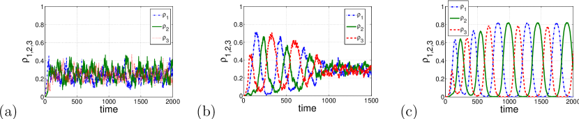
Figure 6: (Color online) Dynamics of the order parameters of three interacting populations of oscillators (parameters like in Fig. 5 (a,c)) for three different sizes of populations: (a) $N=100$, (b) $N=400$, and (c) $N=10000$.

IV.3 Chaotic oscillations

Here we discuss possible “predator-pray”-type regimes (cf. Fig. 2j) for many ensembles. An elementary “oscillator” depicted in Fig. 2j can be represented as a Hamiltonian system with one degree of freedom. Several of such elementary conservative “oscillators”, being coupled, can yield quasiperiodic and chaotic regimes. In the case of two interacting conservative “oscillators” (i.e. of four interacting ensembles), system (7) can be rewritten as follows:

$$\dot{\rho}_{1,2} =\varepsilon_{1,2}\rho_{1,2}(1-D_{0}\rho_{2,1}^{2}-D_{1}\upsilon_{1,2}^{2})(1-\rho_{1,2}^{2})\;,$$ (12)

$$\dot{\upsilon}_{1,2} =\varepsilon_{1,2}\upsilon_{1,2}(1-D_{0}\upsilon_{2,1}^{2}-D_{1}\rho_{1,2}^{2})(1-\upsilon_{1,2}^{2})\;.$$

Here the parameters of the system were chosen in such a way that each pair of subpopulation $(\rho_{1},\rho_{2})$ and $(\upsilon_{1},\upsilon_{2})$ exhibits periodic oscillation being decoupled from another pair (at $D_{1}=0$), i.e. $\varepsilon_{1}\varepsilon_{2}<0$ and $D_{0}>1$. When the coupling between the two pairs is introduced (i.e. $D_{1}\neq 0$), then in dependence on this coupling and initial conditions the dynamics can be qusiperiodic or chaotic. Like in general Hamiltonian systems with two degrees of freedom, it is convenient to represent the dynamics as a two-dimensional Poincaré map. As a Poincaré section (Figure 7a) we have taken the plane $(\upsilon_{1},\upsilon_{2})$ at moments of time at which the variable $\rho_{1}(t)$ has a maximum. At small values of the coupling between the “oscillators” $D_{1}$ the dynamics is typically quasiperiodic. While increasing $D_{1}$, one can observe a transition to dominance of chaotic regimes in the system (12) (see Fig.7a,b and calculation of Lyapunov exponents in Fig.7c). Furthermore, we have confirmed the existence of chaotic oscillations by direct numerical simulation of four subpopulations satisfying (12), consisting of $N=10^{3}$ elements each (Fig.7d).

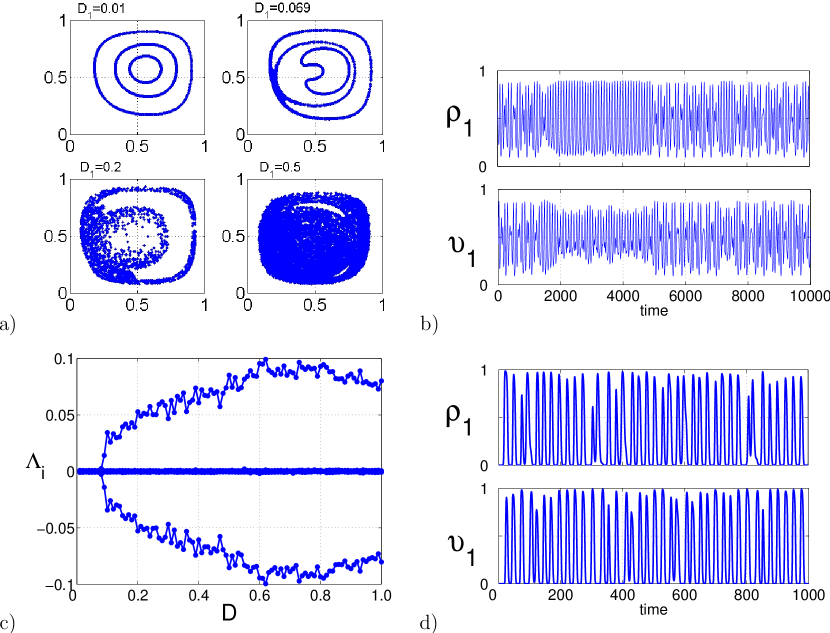
Figure 7: (a) Poincaré sections on the plane $(\upsilon_{1},\upsilon_{2})$ demonstarting regular and chaotic dynamics at different values of $D_{1}$ in the system (12). (b) Time series of a chaotic regime of system (12), for parameter values $D_{1}=0.5$, $D_{0}=2.0$, $\varepsilon_{1}=-1.0$, $\varepsilon_{2}=1.0$. (c) Lyapunov exponents calculated at different values of $D_{1}$, for some particular value of the Hamiltonian. From four Lyapunov exponents two always vanish, while other two vanish for small $D_{1}$ (quasiperiodicity) and are non-zero for larger couling (chaos). (d) Chaotic time series of order parameters of four subpopulations of oscillators consisting of $N=10^{3}$ elements each (the coupling configuration and the parameters are like in panel (b)).

V Conclusion

In this paper we have introduced and studied a model of non-resonantly coupled ensembles of oscillators. It is assumed that oscillators form several groups, in each group the natural frequencies are close to each other, but the frequencies of different groups are rather different. This means that only oscillators within each group interact resonantly (i.e. the coupling terms depend on their phases), while interactions between the groups can be only non-resonant, i.e. depending on slow non-oscillating variables only. As a particular realization of such a setup we considered phase oscillators, which resonantly interact according to the Kuramoto-Sakaguchi model, and the non-resonant terms appear as dependencies of the parameters of the Kuramoto-Sakaguchi model on the amplitudes of the mean fields (Kuramoto order parameters) of other groups.

We employed the Ott-Antonsen theory allowing us to write a closed system of equation for the amplitudes of the order parameters. Analysis of this system constitutes the main part of the paper. The system resembles the Lottka-Volterra type equations used in mathematical ecology for the dynamics of populations, but has nevertheless some peculiarities. For two coupled ensembles we demonstrated a variety of possible regimes: coexistence and bistability of synchronous states, as well as periodic oscillations. For a larger number of interacting groups more complex states appear: a stable heteroclinic cycle and a chaotic regime. Heteroclinic cycle means a sequence of synchronous epochs that become longer and longer. In a chaotic regime the order parameters demonstrate low-dimensional chaos. While the main analysis is performed for the Ott-Antonsen equations that are valid in the thermodynamic limit of infinite number of oscillators in ensembles, we have checked finite-size effects in several regimes by modeling finite ensembles. Finiteness of ensembles only slightly influences the dynamics in most of the observed states, except for the heteroclinic cycle. Here a small effective noise due to finite-size effects destroys the cycle, producing nearly periodic noise-induced oscillations.

One of the models we studied was that of groups of identical oscillators. Here in many cases only the states where some groups completely synchronize (i.e. all oscillators form an identical cluster) while other completely desynchronize (order parameter vanish) are possible. Heteroclinic cycle in this model also connects such states. There is, however, a nontrivial set of parameters, at which the order parameters of ensembles oscillate between zero and one, thus demonstrating time-dependent partial synchronization. Moreover, for four ensembles these oscillations are chaotic. This regime is quite interesting for a general theory of collective chaos in oscillator populations (cf. chaotic dynamics of the order parameter in an ensemble of Josephson junctions reported in Watanabe and Strogatz (1994)) and certainly deserves further investigation.

Appendix A Details of analysis of two interacting ensembles

Here we present details of the analysis of models (8,9), giving the conditions for different regimes presented in Figs. 1, 2.

1. The case of global stability of trivial equilibrium point $S_{1}(0,0),\ M_{1}(0,0)$ (Fig.1a, Fig.2a,b). For system (8) such a situation occurs in the case $\delta_{1,2}<0.$ For system (9) global stability of trivial state $M_{1}$ occurs if $\varepsilon_{1,2}$ are negative and at least one of $D_{12}$ or $D_{21}$ less than 1:

   $$\varepsilon_{1,2}<0,\quad\text{min}(D_{12},D_{21})<1$$ (13)

2. The case of stability of non-trivial state off coordinate axes $S_{4}$ and $M_{4}$ (Fig.1b,c, Fig.2c,d). For system (8) this situation occur in two cases. The first situation appears if $\delta_{1,2}>0$ (when isolated subpopulations tends to synchrony) and suppressive couplings are weak:

   $$\lambda_{1}=\frac{\delta_{2}}{2}\delta_{2}-\delta_{1}d_{21}>0,\qquad\lambda_{2}=\frac{\delta_{1}}{2}\delta_{1}-\delta_{2}d_{12}>0.$$ (14)

   The states $S_{2,3}$ have eigenvalues $-\delta_{1}\delta_{1},\ \lambda_{1}$, and $-\delta_{2}\delta_{2}$, $\lambda_{2}$, respectively, and therefore are saddles. The origin is an unstable node $(\delta_{1,2}>0)$ and therefore the state $S_{4}$ is an attractor (note that $S_{4}$ always exists while (14) holds). We call this situation “case of weak suppressive couplings” because (14) can be written as $d_{12}<\frac{\delta_{1}}{2}\frac{\delta_{1}}{\delta_{2}},\ d_{21}<\frac{\delta_{2}}{2}\frac{\delta_{2}}{\delta_{1}}.$

   The second situation appears if one of the subpopulations approaches to the asynchronous state (negative $\delta$) while another group tends to synchrony and has positive influence on the first subpopulation:

   $$\delta_{1}>0,\ \delta_{2}<0,\ \lambda_{1}>0\ \quad\text{or}\quad\delta_{1}<0,\ \delta_{2}>0,\ \lambda_{2}>0.$$ (15)

   Condition $\lambda_{1}>0$ is equivalent to $d_{21}<\frac{\delta_{2}\delta_{2}}{2\delta_{1}}$, what means that coupling $d_{21}$ should be negative and absolute value of $d_{21}$ should be large enough to maintain partially synchronous state inside the second cluster (positive influence).

   For the system (9) the situation of global stability of $M_{4}$ can be produced by two types of conditions. The first case is that of positive $\varepsilon_{1,2}$ and weak suppressive couplings:

   $$\varepsilon_{1,2}>0,\ D_{12}<1,\ D_{21}<1.$$ (16)

   Another case of global stability of $M_{4}$ occurs if

   $$\varepsilon_{1}<0,\ \varepsilon_{2}>0,\ D_{12}>1,\ D_{21}<1\ \quad\text{or}\quad\varepsilon_{1}>0,\ \varepsilon_{2}<0,\ D_{12}<1,\ D_{21}>1.$$ (17)

   The latter case differs from the previous one only by the direction of the flow on lines $\rho_{1,2}=0$ and the type of unstable points $M_{1},M_{2},M_{3}$ (Fig.2d).

3. The case of competition between subpopulations (Fig.1d,2e). In model (8) this type of behavior arises when

   $$\delta_{1,2}>0,\ \lambda_{1}<0,\ \lambda_{2}<0.$$ (18)

   According to (18) the points $S_{2,3}$ are stable, while $S_{1}$ is unstable node and $S_{4}$ is a saddle. This case corresponds to the situation of strong suppressive couplings

   $$d_{12}>\frac{\delta_{1}}{2}\frac{\delta_{1}}{\delta_{2}},\quad d_{21}>\frac{\delta_{2}}{2}\frac{\delta_{2}}{\delta_{1}}.$$

   Competitive behavior in the system (9) is produced by positive $\varepsilon_{1,2}$ and strong suppressive couplings between subpopulations:

   $$\varepsilon_{0}>0,\ D_{12}>1,\ D_{21}>1.$$ (19)

4. The case of global stability of synchronous state of only one cluster ($S_{2}$,$M_{2}$) (Fig.1e,f,2f,g,h).

   In model (8) only one group is synchronous in two cases. The first trivial situation is similar to conditions (15) (when one group approaches to asynchronous state while another one tends to synchrony) but in this case the active group does not have sufficient positive coupling to maintain synchronization in the asynchronous subpopulation (Fig.1f):

   $$\delta_{1}>0\ \delta_{2}<0\ \lambda_{1}<0\quad\text{or}\quad\delta_{1}<0\ \delta_{2}>0\ \lambda_{2}<0.$$ (20)

   Under conditions (20) only one of the fixed points $S_{2}$ or $S_{3}$ exists and $S_{1}$ is always unstable. The second case occurs at an asymmetric interaction of intrinsically active clusters (isolated clusters tend to synchronous regime):

   $$\delta_{1,2}>0,\quad\text{and}\quad\lambda_{1}<0\ \lambda_{2}>0\quad\text{or}\quad\lambda_{1}>0\ \lambda_{2}<0$$ (21)

   In other words, it appears when one coupling coefficient is strong enough to fully suppress the synchrony in the opponent, for example $d_{21}>\frac{\delta_{2}}{2}\frac{\delta_{2}}{\delta_{1}}$, while another one is weak or even non-suppressing $d_{12}<\frac{\delta_{1}}{2}\frac{\delta_{1}}{\delta_{2}}.$ In this case one can prove that $S_{4}$ does not exist, point $S_{2}$ is a stable node, $S_{3}$ and $S_{1}$ are saddles. Thus all trajectories approach stable node $S_{2}$ which corresponds to the synchronous state of the first group and to the asynchronous state of the second one. Because of this on the plane $(\rho_{1},\rho_{2})$ always exists heteroclinic trajectory connecting saddle point $S_{3}$ and stable equilibrium $S_{2}$ (red line in Fig.1e).

   Global stability of point $M_{2}(M_{3})$ of system (9) occurs in several different cases. The first case is similar to the situation in the system (8) at conditions (20) when one group tends to synchrony ($\delta_{n}>0$), another one approaches trivial state ($\delta_{m}<0$) and synchronous group does not have sufficient positive infuence to maintain synchronization in the asynchronous group:

   $$\varepsilon_{1}<0,\ \varepsilon_{2}>0,\ D_{12}<1\quad\text{or}\quad\varepsilon_{1}>0,\ \varepsilon_{2}<0,\ D_{21}<1.$$ (22)

   Corresponding phase planes are presented in Fig.2g,h. Another case is that of positive $\varepsilon_{1,2}>0$ and asymmetric couplings:

   $$\varepsilon_{1,2}>0,\;D_{12}>1\ D_{21}<1\ \quad\text{or}\quad D_{12}<1\ D_{21}>1.$$ (23)

   Under described above conditions (22), (23) it is easy to show that only one stable fixed point $M_{2}(1,0)$ exists, so all trajectories approach $M_{2}$. In the case of (23) a sequence of heteroclinic orbits connecting $M_{2}$ and $M_{3}$ (red lines in Fig.2f) appears.

5. The case of bistability of trivial and fully synchronous states (Fig.2i).

   In model (9) this happens for negative $\varepsilon_{1,2}$ and strong synchronizing couplings:

   $$\varepsilon_{1,2}<0,\ D_{12}>1,\ D_{21}>1.$$ (24)

6. Periodic behavior (Fig.2j).

   In model (9) periodic solutions can be observed. Conditions

   $$D_{12}>1,\ D_{21}>1,\ \varepsilon_{1}\varepsilon_{2}<0$$ (25)

   provide saddle type of points $M_{1-4}$ and existence of equilibrium $M_{5}$ with imaginary eigenvalues $\pm i\sqrt{\frac{\varepsilon_{1}\varepsilon_{2}(d_{12}-1)(d_{21}-1)}{4d_{12}d_{21}}}.$ Because model (9) can be rewritten as a Hamiltonian one, one has a family of periodic orbits.

References

- Wiesenfeld and Swift (1995) K. Wiesenfeld and J. W. Swift, Phys. Rev. E 51, 1020 (1995).
- Glova (2003) A. F. Glova, Quantum Electronics 33, 283 (2003).
- Kiss et al. (2002) I. Kiss, Y. Zhai, and J. Hudson, Science 296, 1676 (2002).
- Golomb et al. (2001) D. Golomb, D. Hansel, and G. Mato, in Neuro-informatics and Neural Modeling, edited by F. Moss and S. Gielen (Elsevier, Amsterdam, 2001), vol. 4 of Handbook of Biological Physics, pp. 887–968.
- Strogatz et al. (2005) S. H. Strogatz, D. M. Abrams, A. McRobie, B. Eckhardt, and E. Ott, Nature 438, 43 (2005).
- Eckhardt et al. (2007) B. Eckhardt, E. Ott, S. H. Strogatz, D. M. Abrams, and A. McRobie, Phys. Rev. E 75, 021110 (2007).
- Néda et al. (2000) Z. Néda, E. Ravasz, Y. Brechet, T. Vicsek, and A.-L. Barabási, Nature 403, 849 (2000).
- Kuramoto (1975) Y. Kuramoto, in International Symposium on Mathematical Problems in Theoretical Physics, edited by H. Araki (Springer Lecture Notes Phys., v. 39, New York, 1975), p. 420.
- Kuramoto (1984) Y. Kuramoto, Chemical Oscillations, Waves and Turbulence (Springer, Berlin, 1984).
- Daido (1992) H. Daido, Prog. Theor. Phys. 88, 1213 (1992).
- Daido (1993) H. Daido, Prog. Theor. Phys. 89, 929 (1993).
- Daido (1996) H. Daido, Physica D 91, 24 (1996).
- Sakaguchi and Kuramoto (1986) H. Sakaguchi and Y. Kuramoto, Prog. Theor. Phys. 76, 576 (1986).
- Pikovsky et al. (2001) A. Pikovsky, M. Rosenblum, and J. Kurths, Synchronization. A Universal Concept in Nonlinear Sciences. (Cambridge University Press, Cambridge, 2001).
- Acebron et al. (2005) J. A. Acebron, L. L. Bonilla, C. J. P. Vicente, F. Ritort, and R. Spigler, Rev. Mod. Phys. 77, 137 (2005).
- Strogatz (2000) S. H. Strogatz, Physica D 143, 1 (2000).
- Tukhlina and Rosenblum (2008) N. Tukhlina and M. Rosenblum, J. Biol. Phys. 34, 301 (2008).
- Popovych and Tass (2010) O. V. Popovych and P. A. Tass, Phys. Rev. E 82, 026204 (2010).
- Bonilla et al. (1992) L. L. Bonilla, J. C. Neu, and R. Spigler, J. Stat. Phys. 67, 313 (1992).
- Crawford (1994) J. D. Crawford, J. Stat. Phys. 74, 1047 (1994).
- Bonilla et al. (1998) L. L. Bonilla, C. J. P. Vicente, and R. Spigler, Physica D: Nonlinear Phenomena 113, 79 (1998).
- Bonilla (2000) L. L. Bonilla, Phys. Rev. E 62, 4862 (2000).
- Montbrió et al. (2006) E. Montbrió, D. Pazó, and J. Schmidt, Phys. Rev. E 74, 056201 (2006).
- Martens et al. (2009) E. A. Martens, E. Barreto, S. H. Strogatz, E. Ott, P. So, and T. M. Antonsen, Phys. Rev. E 79, 026204 (pages 11) (2009).
- Pazó and Montbrió (2009) D. Pazó and E. Montbrió, Phys. Rev. E 80, 046215 (2009).
- Daido and Nakanishi (2004) H. Daido and K. Nakanishi, Phys. Rev. Lett. 93, 104101 (2004).
- Pazó and Montbrió (2006) D. Pazó and E. Montbrió, Phys. Rev. E 73, 055202 (2006).
- (28) Another novel type of interaction appears if the frequencies of two groups are in a high-order resonance like , see Lück and Pikovsky (2011).
- Rosenblum and Pikovsky (2007) M. Rosenblum and A. Pikovsky, Phys. Rev. Lett. 98, 064101 (2007).
- Pikovsky and Rosenblum (2009) A. Pikovsky and M. Rosenblum, Physica D 238(1), 27 (2009).
- Filatrella et al. (2007) G. Filatrella, N. F. Pedersen, and K. Wiesenfeld, Phys. Rev. E 75, 017201 (2007).
- Giannuzzi et al. (2007) F. Giannuzzi, D. Marinazzo, G. Nardulli, M. Pellicoro, and S. Stramaglia, Phys. Rev. E 75, 051104 (2007).
- Ott and Antonsen (2008) E. Ott and T. M. Antonsen, CHAOS 18, 037113 (2008).
- Ott and Antonsen (2009) E. Ott and T. M. Antonsen, CHAOS 19, 023117 (2009).
- Watanabe and Strogatz (1994) S. Watanabe and S. H. Strogatz, Physica D 74, 197 (1994).
- Pikovsky and Rosenblum (2008) A. Pikovsky and M. Rosenblum, Phys. Rev. Lett. 101, 264103 (2008).
- Murray (2002) J. D. Murray, Mathematical Biology. I. An Introduction (Springer, Berlin, 2002).
- Busse and Clever (1979) F. H. Busse and R. M. Clever, in Recent Development in Theoretical and Experimental Fluid Mechanics, edited by U. Mtiller, K. G. Roessner, and B. Schmidt (Springer, NY, 1979), pp. 376–385.
- Clune and Knobloch (1994) T. Clune and E. Knobloch, Physica D 74, 151 (1994).
- Guckenheimer and Holmes (1988) J. Guckenheimer and P. Holmes, Math. Proc. Camb. Phil. Soc. 103, 189 (1988).
- Krupa (1997) M. Krupa, J. Nonlinear Sci. 7, 129 (1997).
- V. Afraimovich, P. Ashwin, and V. Kirk, Editors (2010) V. Afraimovich, P. Ashwin, and V. Kirk, Editors, A focus issue on Robust Heteroclinic and Switching Dynamics, Dynamical Systems, vol. 25, n. 3 (2010).
- Rabinovich et al. (2001) M. Rabinovich, A. Volkovskii, P. Lecanda, R. Huerta, H. D. I. Abarbanel, and G. Laurent, Phys. Rev. Lett. 87, 068102 (2001).
- Afraimovitch et al. (2008) V. Afraimovitch, I. Tristan, R. Huerta, and M. Rabinovich, CHAOS 18, 043103 (2008).
- Ashwin and Swift (1992) P. Ashwin and J. W. Swift, J. Nonlinear Sci. 2, 69 (1992).
- Hansel et al. (1993) D. Hansel, G. Mato, and C. Meunier, Phys. Rev. E. 48, 3470 (1993).
- Kori and Kuramoto (2001) H. Kori and Y. Kuramoto, Phys. Rev. E 63, 046214 (2001).
- Kori (2003) H. Kori, Phys. Rev. E 68, 021919 (2003).
- Ashwin and Borresen (2004) P. Ashwin and J. Borresen, Phys. Rev. E 70, 026203 (2004).
- Ashwin and Borresen (2005) P. Ashwin and J. Borresen, Physics Letters A 347, 208 (2005).
- Pikovsky and Ruffo (1999) A. Pikovsky and S. Ruffo, Phys. Rev. E 59, 1633 (1999).
- Pikovsky et al. (2002) A. Pikovsky, A. Zaikin, and M. A. de la Casa, Phys. Rev. Lett. 88, 050601 (2002).
- Hildebrand et al. (2007) E. J. Hildebrand, M. A. Buice, and C. C. Chow, Phys. Rev. Lett. 98, 054101 (2007).
- Lück and Pikovsky (2011) S. Lück and A. Pikovsky, Resonancly interacting multifrequency oscillator enesembles, in preparation (2011).