The connection between gamma-ray emission and millimeter flares in Fermi/LAT blazars

We compare the $\gamma$-ray photon flux variability of northern blazars in the Fermi/LAT First Source Catalog with 37 GHz radio flux density curves from the Metsähovi quasar monitoring program. We find that the relationship between simultaneous millimeter (mm) flux density and $\gamma$-ray photon flux is different for different types of blazars. The flux relation between the two bands is positively correlated for quasars and does no exist for BLLacs. Furthermore, we find that the levels of $\gamma$-ray emission in high states depend on the phase of the high frequency radio flare, with the brightest $\gamma$-ray events coinciding with the initial stages of a mm flare. The mean observed delay from the beginning of a mm flare to the peak of the $\gamma$-ray emission is about 70 days, which places the average location of the $\gamma$-ray production at or downstream of the radio core. We discuss alternative scenarios for the production of $\gamma$-rays at distances of parsecs along the length of the jet.

1 Introduction

A relativistic jet is a clear taxonomical characteristic of extragalactic sources detected in $\gamma$-rays. Sources with jets pointing close to our line of sight are called blazars and are the brightest and most dominant population of active galactic nuclei (AGN) in the $\gamma$-ray sky (e.g. Fichtel et al., 1994; Abdo et al., 2010b). The radiation mechanism of the $\gamma$-ray emission in blazars is widely believed to be inverse Compton scattering of ambient photons, either from inside the jet (synchrotron-self-Compton or SSC; e.g. Bloom & Marscher 1986), or from a source external to the jet (external Compton scattering or EC), where the source of seed photons could be the accretion disk (e.g. Dermer & Schlickeiser, 1993), the broad-line region (e.g. Sikora et al., 1994), or perhaps the dusty torus (e.g. Błażejowski et al., 2000). We refer to Boettcher (2010) for a review of theoretical models for blazar emission. Despite all the theoretical modeling efforts, the precise location in general of the $\gamma$-ray emission within sources is still controversial, which in turn makes the origin of the seed photons for inverse-Compton scattering unclear. The proposed models can be roughly divided into two categories: those with $\gamma$-rays originating relatively close to the black hole and the accretion disk, inside the broad-line region (BLR), and those with $\gamma$-rays originating in the radio jet, at distances of several parsecs and well beyond the BLR.

Studies based on data from the EGRET instrument onboard the Compton Gamma Ray Observatory triggered an open debate about the location of the $\gamma$-ray emission site in blazars. The most popular opinion was that $\gamma$-rays are produced within the BLR region via EC (e.g. Sikora et al. 1994). However, other studies found that high levels of $\gamma$-ray emission occurred after the ejections of superluminal jet components (Jorstad et al., 2001), and that $\gamma$-ray detected sources tend to have ongoing high frequency radio flares (Valtaoja & Terasranta, 1995, 1996; Lähteenmäki & Valtaoja, 2003). These results led the authors to conclude that strong $\gamma$-ray emission in blazars was produced in growing shocks in the relativistic jets at parsec-scale distances from the black hole. Well beyond the central BLR, the only source of seed photons appears to be the jet itself, implying that SSC is the main radiation mechanism for the strongest $\gamma$-ray flares in blazars. For a historical perspective of the results obtained during the EGRET era, we refer to Aller et al. (2010)

The dramatically improved $\gamma$-ray data from the Large Area Telescope (LAT) onboard the Fermi Gamma-Ray Space Telescope has opened up the possibility of testing results obtained from the EGRET era regarding the origin of $\gamma$-rays. Several studies, based on the first year of LAT operations, have shown that: (i) the $\gamma$-ray and the averaged radio flux densities are significantly correlated (Kovalev et al., 2009; Giroletti et al., 2010; Ghirlanda et al., 2010; Mahony et al., 2010; Nieppola et al., 2010; Angelakis et al., 2010; Richards et al., 2010; Linford et al., 2011; Arshakian et al., 2011), and (ii) blazars detected at $\gamma$-rays are more likely to have larger Doppler factors (Lister et al., 2009b; Savolainen et al., 2010; Tornikoski et al., 2010) and larger apparent opening angles (Pushkarev et al., 2009) than those not detected by LAT. This observational evidence strongly suggests that radio and $\gamma$-ray emission have a co-spatial origin.

To locate and identify the region where the bulk of $\gamma$-ray emission is produced, and to provide details about its connection to the radio jet, an analysis of simultaneous radio and $\gamma$-ray light curves is necessary. Pushkarev et al. (2010), using data from the MOJAVE survey (Lister et al., 2009a) and the monthly binned $\gamma$-ray light curves provided by the 11-month LAT catalogue (Abdo et al., 2010b), reported that radio flux-density variations lag significantly behind those in $\gamma$-rays, with delays ranging from one to eight months (in the observer’s frame). This suggests that there is a correlation between the parsec-scale radio emission and the strength of the $\gamma$-rays. However, the method employed by the authors did not allow them to clearly characterize the sequence and the structure of individual flares.

Furthermore, we highlight two caveats about the interpretation of radio/gamma correlation analyses, which have often been interpreted too simplistically. First, it is well-known that there is usually a considerable delay between mm and cm radio flares. Thus, although cm-flares would tend to peak after the $\gamma$-ray flares, mm-flares would show shorter delays or possibly even peak before the $\gamma$-rays. The very important second caveat is that a correlation analysis tends to measure the distance between the peaks, especially if the flares have different timescales (as the radio and the $\gamma$-ray flares tend to have). However, a radio flare starts to grow a considerable time before it peaks. The beginning of a millimeter flare coincides with the ejection of a new VLBI component from the radio core (e.g., Savolainen et al. 2002). This is the epoch that must be compared with the $\gamma$-ray flaring, not the epoch of the radio flare maximum. The crucial question is whether a $\gamma$-ray flare occurs before the beginning of a mm-flare, or after it; in the former case the $\gamma$-rays originate upstream of the radio core (the beginning of the radio jet), in the latter, they originate downstream of the radio core, presumably from the same disturbance (i.e. shock) that is visible in the radio regime. (As we discuss in Section 4, the finite length of both the radio core and the disturbance passing through it makes the real situation slightly more complicated. However, the size of the radio core is small compared to its distance from the black hole / accretion disk, and also compared to the distance the newly created disturbance travels during the rise and the peaking of the mm-flare.)

Table 1: The sample of 60 northern radio sources used in this work. Only 45 sources had an adequate decomposition of the total flux density curves at 37 GHz.

Source	Alias	Type	Phase	t${}_{0}^{mm}$-t${}_{peak}^{LAT}$	Distance
				[days]	[$pc$]
(1)	(2)	(3)	(4)	(5)	(6)
0048-097		BLO	0.8	-58.90	…
0059+581		QSO	1.1	-79.32	6.44
0106+013		HPQ	0.4	-63.00	8.94
0109+224	S2 0109+22	BLO	0.6	-28.54	…
0133+476		HPQ	1.1	-62.15	8.36
0212+735		HPQ	1.1	-88.33	1.44
0218+357		QSO	0.9	-74.68	…
0219+428	3C 66	BLO	0.9	-73.08	…
0234+285		HPQ	…	…	…
0235+164		BLO	0.6	-29.03	3.60
0316+413	3C 84	GAL	0.6	-37.50	0.03
0336-019	CTA 026	HPQ	0.8	-55.96	10.18
0420-014		HPQ	0.5	-33.08	3.22
0440-003	NRAO 190	HPQ	0.3	16.36	…
0507+179		QSO	1.1	-76.11	…
0528+134		HPQ	0.6	-34.29	6.45
0716+714		BLO	…	…	…
0736+017		HPQ	1.4	-104.29	10.50
0754+100		BLO	0.6	-44.45	3.54
0805-077		QSO	…	…	…
0814+425		BLO	…	…	…
0827+243	OJ 248	LPQ	1.6	-143.26	20.05
0829+046		BLO	…	…	…
0851+202	OJ 287	BLO	0.1	68.44	11.60
0917+449		QSO	0.5	-30.59	…
J0948+0022		QSO	…	…	…
1055+018		HPQ	0.7	-63.45	3.79
1101+384	MRK 421	BLO	…	…	…
1118-056		QSO	…	…	…
1156+295	4C 29.45	HPQ	1.2	-81.55	28.22
1219+285	ON 231	BLO	1.5	-132.64	…
1222+216	PKS1222+21	LPQ	1.2	-125.24	17.33
1226+023	3C 273	LPQ	1.3	-207.59	35.13
1253-055	3C 279	HPQ	0.8	-50.11	13.46
1308+326		BLO	0.7	-101.08	20.69
1324+224		QSO	…	…	…
1406-076	PKS 1406-07	QSO	1.1	-74.82	…
1502+106	PKS 1502+10	HPQ	1.5	-106.83	5.70
1510-089	PKS 1510-08	HPQ	0.4	-0.98	0.46
J1522+3144		QSO	…	…	…
1606+106		LPQ	1.1	-84.31	15.67
1633+382	4C 38.41	HPQ	1.6	-151.59	30.56
1641+399	3C 345	HPQ	0.4	-34.60	3.95
1652+398	MRK 501	BLO	…	…	…
J1700+6830		QSO	…	…	…
1717+177	PKS 1717+17	HPQ	0.4	-23.63	…
1739+522	S4 1739+52	HPQ	0.7	-65.27	…
1749+096	PKS 1749+096	BLO	1.7	-153.02	10.03
1803+784	S5 1803+784	BLO	…	…	…
1823+568	4C 56.27	BLO	1.2	-317.90	38.39
J1849+6705		QSO	…	…	…
2022-077	PKS 2022-077	QSO	1.0	-74.10	…
2141+175		LPQ	…	…	…
2144+092		QSO	1.8	-483.94	…
2200+420	BL Lac	BLO	0.9	-45.12	2.95
2201+171		QSO	1.7	-170.63	…
2227-088		HPQ	1.1	-66.17	5.06
2230+114		HPQ	1.4	-116.37	11.46
2234+282		HPQ	0.9	-101.39	…
2251+158	3C 454.3	HPQ	0.7	-28.98	8.19

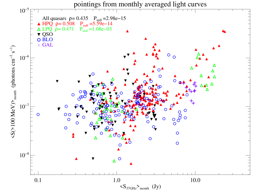
Figure 1: The simultaneous flux - flux relation for the combined sample of 60 radio-loud AGN analyzed here. The different types of sources are symbol coded as shown in the legend. The correlation coefficients are shown only when the significance is $\geq 99.9\leavevmode\nobreak\ \%$

In this paper, we combine the finely sampled 37 GHz Metsähovi light curves and the monthly binned $\gamma$-ray light curves provided by the Fermi/LAT First Source Catalog (Abdo et al., 2010b, 1FGL). By using a radio flare decomposition method, we determine the beginning epochs of millimeter flares (cf. equation 3 in Section 4) and their phases during $\gamma$-ray flaring events to establish the true temporal sequence between $\gamma$-ray and radio flaring. In the following, we use a $\Lambda$CDM cosmology with values within $1\sigma$ of the WMAP results (Komatsu et al., 2009); in particular, H₀=71 km s^-1 Mpc^-1, $\Omega_{m}=0.27$ and $\Omega_{\Lambda}=0.73$.

2 Comparison of Metsähovi and Fermi/LAT  light curves

The Metsähovi quasar monitoring program (Teräsranta et al., 1998) currently includes about 250 AGN at 37 GHz. From them, we selected a sample of sources that fulfill the following criteria: (i) well-sampled light curves during the period 2007-2010, covering the 1FGL period, (ii) a firm association with the 1FGL catalogue, and (iii) a $\gamma$-ray monthly light curve during the 1FGL period that is significantly different from a flat one.

Our final sample consists of 60 sources classified according to their optical spectral type as highly polarized quasars (HPQ, 22), low polarization quasars (LPQ, 5), quasars without any optical polarization data (QSO, 15), BL Lac type objects (BLO, 17), and radio galaxies (GAL, 1). When comparing the averaged radio and $\gamma$-ray properties of the 1FGL sources, and the dependence of the $\gamma$-ray detection likelihood on radio properties, we refer to Tornikoski et al. (2010) and Nieppola et al. (2010). The sample of sources studied in this work is listed in Table 1 along with their spectral types.

To compare radio flux densities and $\gamma$-ray photon fluxes, monthly binned radio light curves were created from the Metsähovi flux density curves at 37 GHz. The time bins are the same as in the 1FGL flux history curves, allowing us to compare simultaneously $\gamma$-ray photon flux and radio flux-density variations with the time resolution of a month. To categorize the phase of the mm flares at the time of the $\gamma$-ray maxima, we decomposed the total flux density variations at 37 GHz into a small number of exponential flares as in previous studies (e.g Valtaoja et al., 1999; Savolainen et al., 2002; Lähteenmäki & Valtaoja, 2003; Hovatta et al., 2009).

3 Results

For each of the 60 sources, we were able to investigate the relation between the $\gamma$-ray photon flux and 37 GHz flux densities during the 11-month 1FGL period. However, only for a subsample of 45 sources did we achieve an adequate decomposition of the total flux density curves, allowing us to categorize in detail the radio flare state during the $\gamma$-ray maxima.

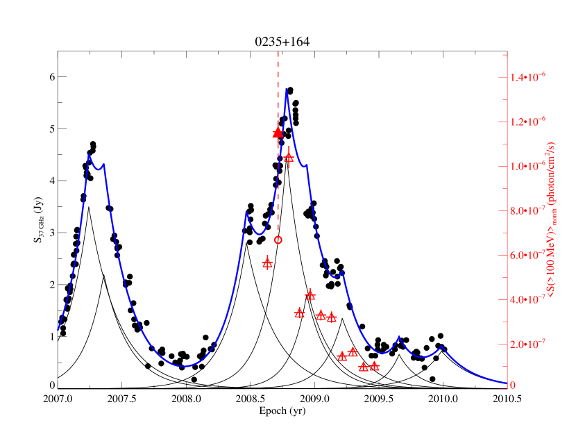
Figure 2: The mm and 1FGL light curves for 0235+164, shown by filled circles and triangles, respectively. The total flux density curve at 37 GHz has been decomposed using individual exponential flares following the method described in Valtaoja et al. (1999). The filled triangle represents the most significant peak in the $\gamma$-ray flux density during the 1FGL period. The dashed vertical line is drawn to highlight the relation between the peak in the $\gamma$-ray light curve and the ongoing millimeter flare.

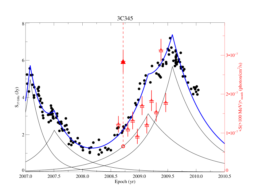
Figure 3: The recent flux history at 37 GHz (filled circles) and $\gamma$-rays (triangles) of 3C 345. The filled triangle represents the most significant peak in the $\gamma$-ray flux density during the 1FGL period, which is clearly associated with a growing shock and a mm flare.

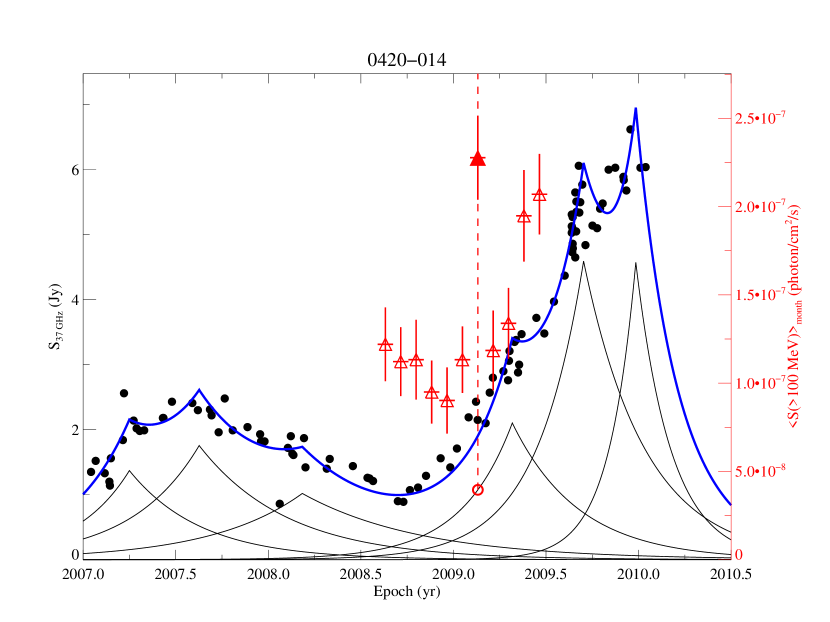
Figure 4: The millimeter and the $\gamma$-ray flux evolution of the highly polarized quasar 0420-014 (PKS 0420-01). A strong millimeter flare is evident after almost two years of quasi-quiescent activity at mm wavelengths, accompanied by a rise in $\gamma$-rays. Although there is a general trend between the mm and gamma ray flux densities, the highest level of $\gamma$-ray emission was reached when the first mm flare was rising (flare phase = 0.5, see Table 1).

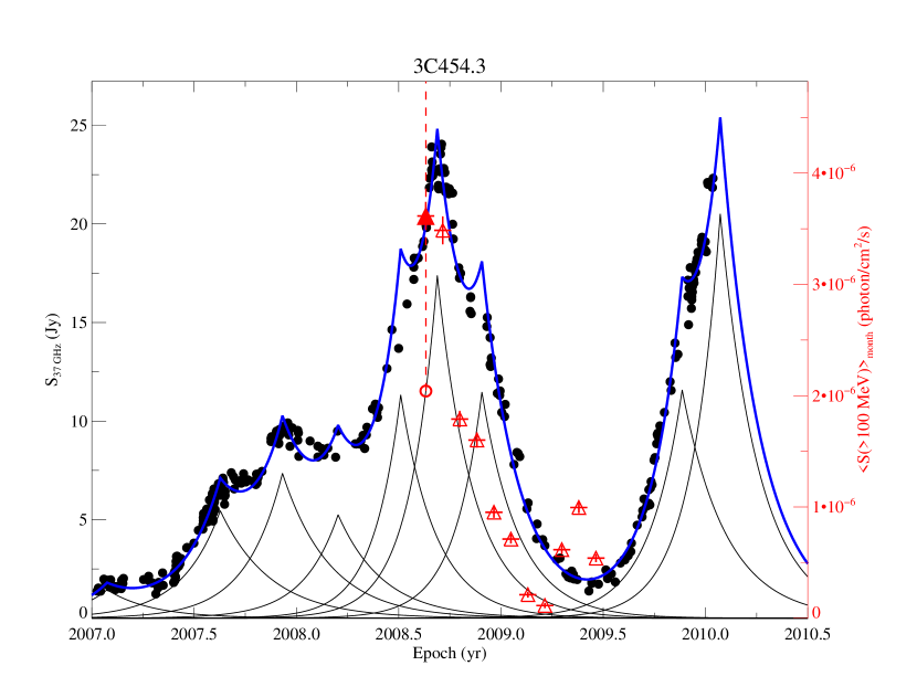
Figure 5: The monthly binned $\gamma$-ray light curve for 3C 345.3. The strongest $\gamma$-ray flux density is reached during the rise of an mm radio flare. Note the weaker $\gamma$-ray flare around 2009.4, discussed in the text. A $\gamma$-ray outburst has been reported in December 2009 (Ackermann et al., 2010), outside the 1FGL period, occurring close to the peak of the latest strong radio flare.

3.1 Simultaneous photon flux - flux density relation

Using the finely sampled light curves from the Metsähovi quasar monitoring program, we compare simultaneous $\gamma$-ray fluxes and 37 GHz flux densities. Figure 1 shows that simultaneous measurements at the two bands appear to be positively correlated. However, we find significant differences between quasars and BL Lacs, which we describe below. By applying the Spearman’s rank correlation test, two very clear results emerge. First, there is a significant positive correlation between the $\gamma$-ray photon flux and the 37 GHz flux density for quasars, while the BL Lac fluxes are not correlated. Second, the strength and the significance of the correlations is different for each type of quasar.

The photon flux - flux density correlation for quasars is absent for QSOs, significant ($\rho=0.47,P_{null}=99.9\%$) for LPQs, and very significant ($\rho=0.50,P_{null}>99.9\%$) for HPQs. Such a dependence on the degree of optical polarization may arise naturally if the polarization indicates the viewing angle of the jet, with sources with high optical polarization having their jets oriented closest to our line of sight (e.g. Hovatta et al., 2009). The dependence of the flux - flux relation on optical polarization agrees with previous results, where it has been shown that the brightest $\gamma$-ray emitters have preferentially smaller viewing angles (Valtaoja & Terasranta, 1995; Lähteenmäki & Valtaoja, 2003) and consequently higher Doppler boosting factors (Lister et al., 2009b; Savolainen et al., 2010; Tornikoski et al., 2010). Since $\gamma$-ray fluxes and radio flux densities are significantly correlated for sources where the relativistic jet is aligned close to our line of sight, this implies that there is a strong coupling between the radio and the $\gamma$-ray emission mechanisms. That the correlation is seen on monthly timescales further indicates a cospatial origin in quasar-type blazars.

Figure 6: The maximum gamma ray flux density versus the radio flare phase (0, beginning; 1 peak; 2 end of the flare). The bottom panel shows the distribution of the flare phases in a boxplot, with the median located at early stages of the flare. Quasars, BLLacs, and radio-galaxies are shown by triangles, circles, and asterisks, respectively.

3.2 Connections between ongoing flares and high states of $\gamma$-ray emission

We decomposed the 37 GHz light curves into individual exponential flares, each of which corresponds to a new disturbance created in the jet that is often detectable as a new VLBI component (Valtaoja et al. 1999, Savolainen et al. 2002). We compared the phase of the individual flares with the $\gamma$-ray light curves obtained from the 1FGL catalogue to determine whether high states of $\gamma$-ray emission are associated with disturbances propagating downstream of the jet.

To identify the maxima in the 1FGL variability flux history, we calculate the derivative at each of the 11 months in the 1FGL period. In this procedure, a peak is a point in the 1FGL curve at which the derivative changes sign. We evaluate, for each peak, the number of points that have a positive derivative at its left plus the number of points with a negative derivative at its right. This is considered as the peak width. The sum of the absolute values of the derivatives for all the points inside the peak width constitutes the peak weight. The larger the weight, the more significant is the peak. To avoid confusion with neighboring peaks not adequately sampled during the 1FGL period, or with flickering, we focus our analysis on the peak with the largest weight (the most significant one) inside the 11 months of the 1FGL period. Hereafter, we refer to the peak with the largest weight as the $\gamma$-ray peak.

Figures 2 to 5 show the 37 GHz total flux density measurements (filled circles) and the 1FGL $\gamma$-ray monthly flux curve (open triangles) for some of the sources included in this study. The individual exponential flares and the total model fits to the flux density curve are shown in Figures 2 to 6 as thin and thick lines, respectively. For each source, we associate the $\gamma$-ray peak with the brightest ongoing radio flare, irrespective of its phase. Such a tie is highlighted by a vertical dashed line connecting the $\gamma$-ray peak (filled triangle) with the brightest individual radio flare (open circle).

Figure 2 shows the source 0235+164. The most significant flare, which also corresponds to the highest observed monthly $\gamma$-ray flux level, occurs just before the peak of the strongest 37 GHz flare. The monthly binned $\gamma$-ray light curve for 3C 345 (Fig. 3) shows two well-defined strong peaks. On the basis of the $\gamma$-ray peak identification method described above, the slightly weaker peak in 2008.7 is more significant than the one considered in the statistical analysis. Nevertheless, it can be seen that both $\gamma$-ray peaks coincide with the rising states of individual radio flares, as in the cases of both 0420-014 (Fig. 4) and 3C 454.3 (Fig. 5). However, around 2009.4 we see a well-defined $\gamma$-ray flare in 3C 454.3, much weaker in intensity, which is not associated with any strong radio flare. This indicates that weaker $\gamma-$ray flares might be produced by mechanisms other than disturbances propagating downstream of the jet, a possibility already suggested in Lähteenmäki & Valtaoja (2003).

Figures 2 to 5 suggest that strong $\gamma$-ray events often occur when a mm radio flare is ongoing, more specifically during the early stages of a mm flare after it has started and is either rising or peaking. However, lacking additional information, we cannot prove a causal connection (i.e., cospatiality) between, say, the strongest gamma and radio flares in 0235+164. What we can do is to look for statistical connections in our sample: do the most significant $\gamma$-ray peaks tend to occur during a specific phase of the radio flares? To quantify the possible connection, the phase of each mm flare has been characterized in the same fashion as in previous works (Valtaoja & Terasranta, 1995, 1996; Lähteenmäki & Valtaoja, 2003), where the phase of a rising flare is defined as

$$\phi_{rising}=S^{\gamma peak}_{mm}/S_{mm}^{max}$$ (1)

and the phase of a decaying flare as

$$\phi_{decaying}=2-S^{\gamma peak}_{mm}/S_{mm}^{max},$$ (2)

where $S^{\gamma peak}_{mm}$ is the flux density of the radio flare at the time of the $\gamma$-ray peak and $S_{mm}^{max}$ is the peak flux density of the radio flare. Equations 1 and 2 correspond to the following characterization of the flares : 0 marks the beginning of the flare, 1 the peak of the flare, and 2 the end of the flare. Thus, a mm flare is growing if its phase ranges between 0 and 1, whereas for any flare phase between 1 and 2 the mm flare is decaying.

We determined the flare phase corresponding to the most significant $\gamma$-ray peak in 45 sources (33 quasars, 11 BL Lacs, and 1 radio galaxy). The values are given in column 4 of Table 1. In Figure 6, we compare the phase of the mm flare at the time of the $\gamma$-ray peak and the flux density of the $\gamma$-ray peak. The top panel gives the distribution of flare phase versus the $\gamma$-ray flux density of the most significant peak during the 1FGL period. At first glance, there appears to be a correlation between the flare-phase and the flux density of the strongest $\gamma$-ray events, suggesting that the strongest $\gamma$-ray peaks tend to occur at the earliest stages of a mm flare. However, the significance of the correlation (P = 80%) is not high enough to be considered as a correlation but only as a trend. Additional Fermi/LAT data will be needed to prove the possible existence of a correlation.

The bottom panel of Figure 6 shows the distribution of the flare phases as a box plot, where the thick line represents the median of the distribution and the box contains 50$\%$ of the sources, delimited by the upper and lower quartiles, whereas the vertical lines indicate the extremes of the flare phases. The median of the radio-$\gamma$-ray events is at the radio phase 0.9, and the majority of the events occur during flare phases between 0.6 and 1.25, indicating that the $\gamma$-ray flares tend to occur during the rising or peaking state of mm flares. This relationship between the flare phase and the $\gamma$-ray maxima is consistent with previous conclusions found from the EGRET data (Valtaoja & Terasranta, 1995, 1996; Lähteenmäki & Valtaoja, 2003).

3.3 Statistical simulations

To assess the statistical significance of the observed flare-phase distribution, we performed the following test. For each source, we performed two random shifts of the monthly binned $\gamma$-ray light curve along the time axis and then measured the corresponding radio phases of the most significant peaks in these shifted $\gamma$-ray light curves, thus creating a random flare-phase distribution. To test whether our observed flare-phase distribution (bottom panel in Figure 6) reveals an intrinsic connection or the distribution is drawn by chance, we start with the assumption that the observed and the random flare-phase distributions are drawn from the same parent distribution and test whether this assumption is valid.

On the basis of the chance assumption, the medians of both distributions should be nearly equal. We mix up all the flare phases from the observed and the random distributions. We then select m of them, which we call ”observed” while the remaining n are designated as ”random”. These new distributions should be almost the same as the original distributions and their median difference should be close to zero. By repeating the procedure 1000 times, we compile a distribution of the differences between the ”observed” and the ”random” distributions. The original median difference between the observed flare-phase and the random flare-phase distribution is -0.93. By using the distribution built on 1000 permutations, we compute the p-value for the probability of obtaining a median difference larger (in terms of absolute value) than the observed one. The p-value computed is 0.005, which leads us to conclude that the observed flare-phase distribution (shown in the bottom-panel of figure 6) is not drawn by chance at a significance level of $99.5\%$ . To help implement these statistical simulations, we used the permutation routines of the statistical R language and our IDL routines.

Figure 7: Top panel: The distribution of the observed delays between the beginning of a mm flare ($t_{0}^{mm}$) and the peak in the 1FGL light curves ($t_{peak}^{LAT}$). The mean observed delay is about 70 days, with radio leading the $\gamma$-rays. The delays for each individual source have also been estimated in the source frame and the distribution is shown in the bottom panel. The mean value of the delay in the source frame is roughly one month.

4 The location of the $\gamma$-ray emission site

The results described in the previous section show that mm flux densities and gamma ray fluxes in sources with optical polarized emission (HPQ, LPQ) are correlated on monthly timescales, whereas for both quasars without polarization data (QSO) and BL Lacs (BLO) such a correlation is not found. Although the inverse Compton mechanism predicts a correlation between radio and $\gamma$-ray emission strengths, studies from the EGRET era did not find evidence of this correlation (e.g. Lähteenmäki & Valtaoja, 2003). This apparent contradiction with results obtained here is probably due to the limited EGRET sensitivity and to the sparse $\gamma$-ray data available at that time. The absence of $\gamma$-ray and radio flux density correlation for BL Lacs might be an indication that $\gamma$-ray emission mechanisms or locations are different for quasars and BL Lacs (Lähteenmäki & Valtaoja, 2003). In quasars, $\gamma$-rays and radio flux densities are most significantly correlated for sources with the relativistic jet pointing close to our line of sight (HPQs), which implies that there is a strong coupling between the radio and the $\gamma$-ray emission mechanisms. That the correlation is seen in monthly flux density levels may imply that they have a co-spatial origin.

Perhaps the most remarkable result is that the most significant $\gamma$-ray flux peaks occur when a mm-flare is either rising or peaking. As discussed in Section 1, this indicates a sequence of events where first a disturbance (i.e. shock) emerges from the radio core, becoming visible as an increase in the mm radio flux (and as a new VLBI component, (Jorstad et al., 2001)), and after that the $\gamma$-ray flux rises and peaks. In other words, strong $\gamma$-ray flares are produced in the same disturbances that produce the mm flares, downstream of the radio core in the relativistic radio jet. Using our data, we can estimate the time delay between the time when the mm flare starts and when the $\gamma$-rays peak for each source. We define the beginning of a mm flare to be:

$$t_{0}^{mm}=t_{max}^{mm}-\tau,$$ (3)

where $t_{max}^{mm}$ is the time of the mm flare peak and $\tau$ is the variability timescale (Savolainen et al., 2002; Lähteenmäki & Valtaoja, 2003). In other words, we define the beginning of the flare as the epoch when its flux is 1/e of the maximum flux.

In the top panel of Figure 7, we plot the distribution of the observed time delays. As can be seen, the distribution is centered around 70 days with the beginnings of the radio flares preceding the $\gamma$-ray peaks, which agrees with results obtained during the EGRET era. Lähteenmäki & Valtaoja (2003) found time lags between 30-70 days from the onset of a millimeter flare to the $\gamma$-ray flare, and Jorstad et al. (2001) found a mean time lag from the VLBI ejection time to the $\gamma$-ray flare to be 52$\pm$76 days. In the bottom panel of Figure 7, we show the distribution of the delays in the source frame, with a median delay of 30 days.

To locate the maximum $\gamma$-ray production region, we can convert the time delays to linear distances from the region where the mm outburst begins (i.e., the radio core, as we argue below) to the region of the $\gamma$-ray production by using the expression (e.g. Lähteenmäki & Valtaoja, 2003; Pushkarev et al., 2010)

$$\Delta r=\frac{\beta_{app}c(t_{0}^{mm}-t_{peak}^{LAT})}{sin\theta\leavevmode\nobreak\ (1+z)},$$ (4)

where $\theta$ and $\beta_{app}$ are the jet viewing angle and the apparent jet speed, respectively. By taking the latter values from the MOJAVE website and using the delay computed in this work, we were able to compute the linear distance from the radio core to the region of the $\gamma$-ray production for 30 sources in our sample. These values are given in Table 1.

If we consider only those sources for which the $\gamma$-ray peak occurs when a mm flare is rising or peaking ($0\leq phase\leq 1.25$), then an outlier-resistant determination of the mean leads us to conclude that in our sample the average location of the $\gamma$-ray emission site is $\langle R_{\gamma}\rangle=7.4\pm 1.3\ pc$ downstream from the radio core, which places the $\gamma$-ray emission site well outside the canonical BLR ($\leq 1pc$), even without taking into account that the radio core itself is at a considerable distance from the black hole. A contemporaneous estimate of the location of the $\gamma$-ray emission site for 3C  279 (about $10^{5}$ gravitational radii, Fermi-Lat Collaboration et al., 2010) is in good agreement with the distance reported in Table 1 (13.4 pc $\sim 2\times 10^{5}$  R_S, assuming a black hole mass of 6 $\times 10^{8}$ M_☉). Furthermore, Agudo et al. (2011) found that the $\gamma$-ray emission in OJ 287 is generated in a stationary feature located at a distance $>14\leavevmode\nobreak\ pc$ from the central engine, which is also consistent with the distance derived in this work ($\sim 12\leavevmode\nobreak\ pc$). For 3C 345, Schinzel et al. (2010) find that $\gamma$-rays are produced up to 40 pc from the engine, which is again consistent with our finding of an emission site downstream of a radio core, itself at a considerable distance from the black hole.

We note that we have compared the time delay at the beginning of the radio flare with that at the peak of the $\gamma$-ray flare, whereas ideally we should compare the beginnings of both. At present, these Fermi $\gamma$-ray data are unavailable. However, it is well known from both EGRET observations and the Fermi data analyzed here that the strongest $\gamma$-ray flares tend to have a short duration, with typical timescales of a month or less (see also Figs. 3 and 4). The delays from the onsets of the mm-flares to the onsets of the $\gamma$-ray flares are therefore somewhat shorter than those shown in Fig. 7, but the temporal order of events is unchanged.

A number of other studies have also found that the radio core is located parsecs or even tens of parsecs away from the central engine. A partial list includes Jorstad et al. (2007), Chatterjee et al. (2008), Marscher et al. (2008), Sikora et al. (2008), Jorstad et al. (2010), and Marscher et al. (2010). Thus, any correlation between $\gamma$-ray flares and radio events (millimeter flares, VLBI ejections) implies a ”distant” origin scenario, with $\gamma$-rays produced far beyond the BLR, in the vicinity of the radio core situated around $10^{5}$ R_S, or downstream from it.

However, before we can claim that all $\gamma$-ray flares are generated at distances of parsecs downstream of the radio core, we recall the following two caveats:

1. Our results refer only to the most prominent $\gamma$-ray peak in the 1FGL light curves. For many sources in our sample, the 1FGL light curve displays several other flares, such as the one around the middle of 2009 in Figure 5. It is striking that this flare occurred during a period of quiescent mm-activity. It is possible that these smaller flares in quasars, and flares in general in BL Lacs, are produced by a different mechanism or at different locations, most likely upstream of the radio core.
   

2. Monthly bins in the 1FGL curves might mask rapid $\gamma$-ray flares, or blend them with each other. However, even if some of our ”most significant” flares result from a superimposition of two or more rapid flares, the time difference between them must be smaller than the delays found in Table 1, and our basic argument about the connection to the radio core remains valid. The analysis of rapid $\gamma$-ray flares is beyond the scope of this paper, but we note that significant efforts in this direction have already been made (Marscher et al., 2010; Tavecchio et al., 2010).

Despite the above caveats, no argument conflicts with our main conclusion, namely, that strongest $\gamma$-ray flares tend to occur at initial or peaking stages of a mm flare and that they are therefore related to disturbances (i.e. shocks) propagating downstream from the core. However, both the radio core and the disturbances have finite lengths, which complicates the interpretation. There is no commonly accepted physical model for either the radio core or the shocked jet flow, but we can consider the following general scenario, in which a finite-length disturbance passes through an extended radio core. We refer to Figure 9 of Marscher (2009) for a pictorial representation of the AGN structure assumed here. There are three stages during which $\gamma$-rays may be produced.

1. Upstream of the radio core: Once a disturbance is produced close to the black hole and the accretion disk, it traverses downstream along the so-called acceleration and collimation zone (ACZ) (Marscher et al., 2008). The accretion disk and the BLR are copious sources of seed photons, which, however, diminish quickly as the disturbance approaches the radio core at the distance of several parsecs (of the order of $10^{5}$ R_S). Eventual $\gamma$-ray flaring should clearly precede any radio events. For example, for 3C 279 Chatterjee et al. (2008) find that X-rays, presumably generated close to the central engine, lead radio variations by 130 days. For $\gamma$-rays created from accretion disk or BLR seed photons (the ”near” origin scenario), comparable delays to radio variations should be seen.
   

2. Passing through the radio core: After the ACZ, the disturbance reaches a recollimation or standing conical shock (Daly & Marscher, 1988; Gomez et al., 1995), which can be most readily identified in VLBI maps with the brightest stationary feature, the so-called radio core. The radio emission presumably starts to rise as the moving disturbance enters the radio core. By definition, the VLBI ejection epoch, determined by extrapolating the component motion backwards in time, should occur when the disturbance passes the center of the radio core. The relative temporal sequence of mm-flare onset, VLBI ejection epoch, and possible $\gamma$-ray flaring depend on the as yet unknown physics of shock inception and growth. However, owing to the relatively small size of the radio core no large delays between core-related events are expected. According to Marscher (2009), the size of the radio core can be approximated as $a_{core}=0.05(43GHz/\nu_{m})$ milliarcsec, where $\nu_{m}$ is the frequency at which the core becomes self-absorbed. Assuming $\nu_{m}=43$ GHz for a typical source in our sample ($<z>\sim 0.8$, $\beta_{app}\sim 11.1$, $\theta\sim 3^{\circ}$), then the passage time of a disturbance through the core ($a_{core}\sim 0.05$ mas) is about 70 days, which is similar to the mean time-delay from the onset of a mm flare to the $\gamma-$ray peak ($\sim$2 months). However, it must be borne in mind that the core size here is an upper limit estimated from model fitting the unresolved stationary component associated with the core on VLBI images and may be much larger than the actual size of the radio core. In addition, we do not know if the millimeter flare begins as the disturbance enters the radio core, or first later, as opacity and shock physics are likely to play a role.
   

3. Downstream of the radio core: As the shock emerges from the core, it becomes detectable in VLBI maps as a new component. According to Hovatta et al. (2008), the median rise time for a 37 GHz flare is one year, indicating that the shock traverses a considerable distance downstream from the radio core before it enters its final adiabatic decay phase. For $\gamma$-rays originating in shocks, time delays longer than in case (ii) are expected. We note again that a delay of months or even longer from the $\gamma$-ray flare to the peak of the radio flare does not imply that the origin is the radio core, and much less in the vicinity of the central engine.

Our main finding, that the most intense $\gamma$-ray flares in the 1FGL light-curves occur about 70 days after the onset of a mm flare, indicates a ”distant” origin scenario, with emission sites located several parsecs away from the central engine. In this scenario, corresponding to cases (ii) and (iii), the highest levels of $\gamma$-ray emission are achieved during, or after, the passage of the disturbance through the core (or through an outer stationary feature), thus compressing the moving material and enhancing substantially the energy of electrons, leading to the inverse Compton scattering of low-energy photons provided either by the jet itself or from external photon fields.

The two-month average delay we find is most consistent with cases (ii) and (iii), however, for several reasons we cannot decide on whether the strongest $\gamma$-ray flares occur during disturbances passing through the radio core (case (ii)) or if they originate from the growing shocks downstream of the radio core (case (iii)). First, our time resolution of one month is insufficient for detailed studies of the sequence of events during the passage of the disturbance through the radio core. Second, as can be seen in Figure 7, the spread in the lengths of the delays is not inconsiderable. Third, we have defined the beginning of the radio flare using a simple formula (Equation 3), which obviously is an approximation. Inspection of individual mm-flares in the Metsähovi monitoring program reveals that in several cases the radio flux starts to increase somewhat before or after the epoch given by Equation 3. Multifrequency monitoring, preferably combined with VLBI and time-resolved $\gamma$-ray light curves, is needed to achieve more accurate time determinations and studies of case (ii).

For the strongest $\gamma$-ray flares, case (i) seems to be excluded by our results, although our time resolution cannot exclude the possibility that some of the flares are produced a short distance (as compared to the distance to the central engine) upstream of the radio core. However, we should also remain open to the possibility that $\gamma$-ray flares are generated close to the black hole due to an enhancement of the local seed photons (either from the accretion-disk corona system or the canonical BLR), as has been suggested in other studies (e.g. Marscher et al., 2010; Tavecchio et al., 2010). Nevertheless, $\gamma$-ray flares produced in the close dissipation scenario ($\leq 1$ pc) should, in general, occur months before the mm-flare inception and the VLBI component ejection. Whether close-dissipation $\gamma$-ray flares are related to weak and/or rapid flares will be addressed in a future work by means of high-resolution $\gamma$-ray light curves.

In conclusion, the results presented in this paper strongly indicate that at least for the strongest $\gamma$-rays the production sites are downstream or within the radio core, well outside the BLR at distances of several parsecs or even tens of parsecs from the black hole and the accretion disk. A number of papers based on Fermi data have reached similar conclusions, mainly for individual sources (e.g. Fermi-Lat Collaboration et al., 2010; Schinzel et al., 2010; Agudo et al., 2011). In particular, Pushkarev et al. (2010) have also studied a large sample of sources statistically, concluding that the $\gamma$-ray production takes place within the extended radio core. The finding that $\gamma$-rays lead the radio emission by 1.2 months (in the source frame), which is consistent with our results when we take into account the average time delays between 37 GHz and 15 GHz and that they compared the peak times, not the beginnings of the radio flare as we have done (cf. Section 1).

In the current AGN paradigm, the sources of seed photons to produce $\gamma$-rays at distances well beyond the canonical BLR could be provided by (a) the dusty torus (e.g. Błażejowski et al., 2000) or (b) by the jet itself, either via a slow sheath surrounding the fast spine of the jet (Ghisellini et al., 2005), or from the same disturbances that produce the radio outburst. Firm detections of IR emission associated with a hot dusty torus have so far been limited to a couple of bright blazars (Türler et al., 2006; Malmrose et al., 2011), and, as is well known, SSC models in general fail to produce the observed amounts of $\gamma$-ray emission, assuming physically reasonable parameter values for the shocked regions. However, León-Tavares et al. (2010) and Arshakian et al. (2010) have shown that radio-loud sources with superluminal motions may power an additional component of the BLR, which can be located parsecs downstream of the canonical BLR ($<1\leavevmode\nobreak\ pc$). In effect, the flow drags a part of the BLR with it. Based on these results, a tentative idea to test is whether an outflowing BLR can serve as a source of external photons to produce $\gamma$-rays, even at distances of parsecs down the jet . In this scenario, the strong $\gamma$-ray events are produced in the shocks of the jet by upscattering external photons provided by the outflowing BLR. Although a combination of optical spectral-line monitoring with regular VLBA observations has strongly suggested that an outflowing parsec-scale BLR is present (León-Tavares et al., 2010; Arshakian et al., 2010), it is obviously of greatest importance to extend these observations to many more objects to explore the feasibility of producing $\gamma$-rays far downstream of the central engine and the radio core by means of EC radiation mechanisms.

The most effective way to explore the above scenario (and others) is by modeling simultaneous, well-sampled spectral energy distributions (SEDs). Although these high quality SEDs are quite expensive in terms of manpower and observing time, significant progress has already been made (e.g. Abdo et al., 2010a). Even higher quality SEDs are becoming available from Planck, Swift, and Fermi satellites and supporting ground-based observatories (Planck Collaboration et al., 2011). Furthermore, the black hole mass is a crucial parameter that controls the accretion rate. It is also found that the more massive the black hole is, the faster and the more luminous jet it produces (Valtaoja et al., 2008; León-Tavares et al., 2011). Thus, a reliable estimate of the black hole masses is an essential input to theoretical models of both the shape and the variability of blazars SEDs.

5 Conclusions

We have compared monthly $\gamma$-ray light curves with the finely sampled Metsähovi 37 GHz light curves of northern sources identified in the 1FGL, finding that:

1. A significant correlation exists between simultaneous $\gamma$-ray photon fluxes and 37 GHz flux densities in quasars, more specifically, among those with high optical polarization. The absence of any similar correlation for BL Lacs might indicate that different $\gamma$-ray emission mechanisms operate in quasars and BL Lacs.
   

2. Statistically speaking, the strongest $\gamma$-ray flares occur during the rising /peaking stages of millimeter radio flares. This result supports the scenario where the $\gamma$-ray emission in blazars originates in the same disturbances in the relativistic plasma (i.e. shocks) that produce the radio outbursts, around, or more likely downstream, of the radio core and far outside the classical BLR.
   

3. The average observed time delay from the onset of the millimeter flare to the peak of the $\gamma$-ray flare is 70 days, corresponding to an average distance of 7 parsecs along the jet. At these distances, well beyond the canonical BLR, the seed photons could originate either from the jet itself, from a dusty torus, or from an outflowing BLR. The existence of a nonvirial, outflowing BLR can make EC models possible even at distances of parsecs down the jet.