Detection of Majorana edge states in topological superconductors through the non-Fermi-liquid effects induced in an interacting quantum dot

Abstract

It is shown that the presence of the continuum of Majorana fermion edge states along the perimeter of a chiral topological superconductor can be probed using an interacting quantum dot coupled to three terminals: the lead supporting the Majorana edge states and two spin-polarized (ferromagnetic) measurement leads. The hybridization with the Majorana states induces a particular type of the Kondo effect with non-Fermi-liquid properties which can be detected by performing linear conductance measurements between the source and drain measurement leads: the temperature and magnetic-field dependence of the conductance is characteristically different from that in the conventional Kondo effect.

I Introduction

Two-dimensional (2D) electron systems with gapped bulk states and gapless edge states have been intensely studied ever since the discovery of the quantum Hall effect von Klitzing et al. (1980) and the emergence of the theories which brought to light the topologically non-trivial nature of the quantum Hall state Thouless et al. (1982). In recent years, this line of research has significantly intensified with the prediction and the subsequent experimental discovery of the time-reversal-invariant generalizations of the quantum Hall state where the role of the external magnetic field is played by the strong spin-orbit coupling Kane and Mele (2005); Fu and Kane (2006); Bernevig and Zhang (2006); Moore and Balents (2007); Bernevig et al. (2006); König et al. (2007). These systems, now known as the “two-dimensional topological insulators”, are insulating in the bulk but support helical edge states, i.e., a pair of one-dimensional propagating modes connected by the time-reversal symmetry (Kramers’ pairs) and propagating in the opposite directions for the opposite (pseudo)spins Bernevig and Zhang (2006). The edge states have dispersion along the edge, but they are confined along the direction perpendicular to the edge. These states are robust against perturbations which preserve the time-reversal (TR) invariance, since their presence is guaranteed by the non-trivial topological properties of the bulk states. In addition to 2D topological insulators (TI), there are also three-dimensional TIs with insulating bulk states and topologically protected gapless chiral surface states, which have Dirac spectrum. Such materials are also known as “strong topological insulators”.

In a metal with a Dirac spectrum Majorana fermion bound states can be induced by the s-wave superconductivity through the proximity effect Bergman and Hur (2009); Nilsson et al. (2008). Majorana fermions can be described as real fermions ($\eta^{\dagger}=\eta$) and have half the degrees of freedom as the complex Dirac fermions. In other words, a set of fermionic creation and annihilation operators can be rewritten using a pair of Majorana operators as $\psi=(\eta_{1}+i\eta_{2})/\sqrt{2}$ and $\psi^{\dagger}=(\eta_{1}-i\eta_{2})/\sqrt{2}$. This is more than a simple change of basis, since Majorana states may be spatially separated. Especially important are the situations where the Majorana modes have zero energy, as this implies the degeneracy of the ground state Ivanov (2001) and it allows the system to support excitations with non-Abelian statistics (i.e., particles which are neither fermions nor bosons) Stern (2010). Such systems would allow reliable non-local storage of quantum information Kitaev (2001) and they would provide the building blocks for topological quantum computers Kitaev (2003). While the non-Abelian states of matter have not been observed yet, there is now an intensive search for Majorana excitations in various condensed-matter systems Wilczek (2009); Stern (2010).

As the dispersion of the surface-state electrons on a strong TI forms a Dirac cone, an interesting state has been predicted to emerge by bringing in contact a TI with an (s-wave) superconductor Fu and Kane (2008). A linear junctions between a superconductor and a magnet in contact with a TI may namely form a one-dimensional wire for Majorana fermions Fu and Kane (2008, 2009a). Such a “Majorana quantum wire” can be described as “half a regular 1D Fermi gas” Fu and Kane (2008). A number of related systems may also support Majorana edge modes: regular semiconductors with spin-orbit coupling in proximity to a superconductor and a magnetic insulator Sau et al. (2010a, b), edge states of 2D TIs Fu and Kane (2009b), junctions with ferromagnetic insulators Tanaka et al. (2009), etc.

Unfortunately, Majorana fermions are by their very nature rather elusive and it is difficult to assert their existence in a given system. Majorana fermions in superconductors are electrically neutral and do not couple to external fields. One approach for their detection has been, for example, to combine two Majorana fermions into a single Dirac fermion in order to allow probing with charge transport Fu and Kane (2009a); Akhmerov et al. (2009). Various detection schemes have already been proposed for Majorana modes in topological insulators. Some of them are only capable of detecting the presence of Majorana modes (either single localized levels or continua of propagating modes), while others can actually measure the state of the system (they are, thus, read-out schemes) and could be used to demonstrate the non-Abelian statistics associated with the Majorana zero-energy modes. The detection schemes are based on the detection via the Josephson current Fu and Kane (2009b), on interferometry Fu and Kane (2009a); Akhmerov et al. (2009); Law et al. (2009); Sau et al. (2010c), “teleportation” (non-local electron transfer process which maintains the phase coherence) Fu (2010), flux qubit interferometry Hassler et al. (2010), or noise measurements Nilsson et al. (2008).

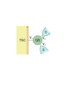
Figure 1: (Color online) An interacting quantum dot QD is coupled to a spin-up Majorana fermion edge channel of a chiral topological superconductor TSC with hopping $V_{T}$ and to two ferromagnetic probe leads (source S and drain D electrodes) which are fully spin polarized in the spin-down direction with hoppings $V_{S}$ and $V_{D}$. Instead of ferromagnetic probe leads, one may also use two systems in the quantum anomalous Hall state which have fully spin-polarized edge states. The hybridization with the Majorana modes localized along the perimeter of the topological superconductor will induce a non-Fermi-liquid Kondo effect which can be probed using the ferromagnetic contacts by measuring the temperature dependence of the (spin-down) linear conductance through the dot. To tune the system to the non-Fermi-liquid point, one can change the gate voltage on the dot, apply an external magnetic field, and change the coupling constants $V_{S}$, $V_{D}$ and $V_{T}$. Dashed line denotes Majorana electrons, full line indicates Dirac electrons, while the shades of gray (colors online) distinguish spin-up and spin-down polarization.

In this paper a further Majorana mode detection scheme is described. It is a simple detection scheme, not a read-out scheme. It makes use of the effect of the Majorana modes on the screening of the impurity spin if an interacting quantum dot is coupled to the Majorana quantum wire on one side and to two normal (but spin-polarized) measurement wires on the other side, as shown in Fig. 1. The idea here is that Majorana fermions and the non-Fermi-liquid variants of the Kondo effect (for instance, the two-channel Kondo effect, which is relevant here) go hand in hand. It will be shown that the coupling of the quantum dot to an additional Majorana mode will modify the transport properties of the quantum dot probed by the additional leads. In particular, it will change the temperature dependence of the linear conductance. Some aspects of the proposed scheme are related to the work on quantum dots coupled to the edge states of the $\nu=5/2$ fractional quantum Hall effect (FQHE) Fiete et al. (2008, 2010); Sevier and Fiete (2011). The two cases differ in the origin of the degrees of freedom which are necessary (in addition to the Majorana modes) to generate the two-channel Kondo effect: in the FQHE, they are the bosonic edge states [field $\phi$ in Eq. (1) in Ref. Fiete et al., 2008], while here we make use of the spin-polarized probing leads. The two cases also differ in the measurement scheme: in the FQHE case, one measures the charge susceptibility of the dot using capacitively coupled probes, while here we propose to perform transport experiments.

The description of the generalized Kondo problems with non-Fermi-liquid fixed points in terms of Majorana modes has been very fruitful and it allows for a simple interpretation of the finite-size excitation spectra Maldacena and Ludwig (1997); Bulla et al. (1997). A well known example is the two-channel Kondo (2CK) effect which has been intensively discussed theoretically Nozières and Blandin (1980); Sacramento and Schlottmann (1991); Pang and Cox (1991); Affleck and Ludwig (1992); Emery and Kivelson (1992); Sengupta and Georges (1994); Andrei and Jerez (1995); Ye (1996); Cox and Zawadowski (1998); Zaránd and von Delft (2000); Zaránd et al. (2002) and was recently experimentally realized using semiconductor quantum dots Potok et al. (2007). This type of the Kondo effect occurs when a single spin-$1/2$ quantum impurity is equally coupled to two independent screening channels (there must be no charge transfer between the channels Žitko and Bonča (2007); Zaránd et al. (2006)); this leads to an overscreening effect in which the localized spin forms a new spin-$1/2$ state by coupling to two neighboring spins from the leads, this new spin-$1/2$ collective state is then coupled to the two next-nearest neighbor spins from the leads into another spin-$1/2$ state, and so forth, generating a complex non-local screening cloud state. The non-Fermi-liquid state associated with the two-channel Kondo effect can be described using conformal field theories in which an odd number of Majorana modes have their boundary conditions twisted due to the presence of the magnetic impurity Maldacena and Ludwig (1997).

Quantum impurities (either in the form of quantum dots or magnetic impurity atoms) in contact with topological insulators have already been studied in different contexts. The Kondo effect due to a magnetic impurity in the helical edge liquid may be affected by the interactions in the one-dimensional chiral channel Maciejko et al. (2009), although the experiments indicate that the interactions in known systems appear to be rather weak, with a Luttinger parameter $K\sim 1$ König (2007); Maciejko et al. (2009). For a quantum dot coupled to two helical edge states a variant of the two-channel Kondo effect may occur Law et al. (2010). It has also been shown that a quantum impurity coupled to Majorana edge fermions Shindou et al. (2010) may be mapped to a two-level system with Ohmic dissipation. This last problem is somewhat related to the one discussed in this work, but there is crucial difference: the model proposed here allows particle exchange with the Majorana wire, while the model studied in Ref. Shindou et al., 2010 considers only the exchange coupling (without discussing its microscopic origin). As commonly observed in other impurity problems, an exchange-only effective model may behave rather differently than a model with hopping terms; this appears to be the case here, too.

We discuss a quantum dot coupled to a Majorana channel on one side and two spin-polarized leads on the other. When the spin-polarization of the probe leads is opposite to that of the Majorana channel, the impurity couples to three Majorana modes, while the fourth mode of the full Anderson impurity model is absent (or fully decoupled). It has to be emphasized that the spin-polarized leads are not only “probe” leads to measure the transport properties of the system, but they are crucial for the emergence of the (two-channel) Kondo effect, i.e., they participate in the formation of the Kondo state. The full details of the model considered will be presented in Sec. II, where the numerical techniques will also be briefly described. The results of numerical calculations will be given in Sec. III and we conclude with a brief discussion of the possible issues in the experimental realization of the proposed scheme. In an Appendix, we solve exactly the non-interacting resonant-level model with different couplings to the Majorana modes of a single conductance channel.

II Model and method

For definiteness, we consider the physical realization of a system supporting a one-dimensional Majorana edge channel as proposed in Ref. Qi et al., 2010. The system is a hybrid device made of an insulator layer in the quantum anomalous Hall (QAH) state and a fully gapped superconducting layer. Its phase diagram supports a chiral topological superconductor (TS) phase with an odd number of chiral Majorana edge modes Qi et al. (2010). The QAH state can be induced by magnetic doping of topological insulators Liu et al. (2008); Yu et al. (2010); Qi et al. (2010): as the magnetization increases, the spin down (for example) edge states penetrate deeper in the bulk until they disappear by merging with the bulk states, while the spin up edge states remain bound to the edge. The QAH system thus has spin-polarized single chiral edge states. When this system then experiences the superconducting proximity effect, it may be tuned to become a TS Qi et al. (2010). The single edge mode decomposes into two chiral Majorana edge modes, one of which penetrates deeper in the bulk and disappears, while the remaining one persists bound to the edge Qi et al. (2010). We are thus left with a single spin-polarized (we choose it as spin-up) chiral Majorana fermion edge state, with the effective Hamiltonian

$$H_{\mathrm{edge}}=\sum_{p>0}vp\left(\eta_{-p}\eta_{p}\right),$$ (1)

where $v$ is the Fermi velocity, $p$ the momentum, and $\eta_{p}$ the Majorana fermion operators which satisfy the canonical Majorana anticommutation rules $\{\eta_{p},\eta_{p^{\prime}}\}=\delta_{p,p^{\prime}}$.

The quantum dot is described as a single impurity level $d$:

$$H_{\mathrm{dot}}=\sum_{\sigma}\epsilon n_{\sigma}+Un_{\uparrow}n_{\downarrow}+g\mu_{B}B\frac{1}{2}\left(n_{\uparrow}-n_{\downarrow}\right).$$ (2)

Here $n_{\sigma}=d^{\dagger}_{\sigma}d_{\sigma}$ is the spin-$\sigma$ occupancy operator, the energy level $\epsilon$ can be controlled by the gate voltage, $U$ is the on-site charge repulsion, $g$ is the gyromagnetic ratio, $\mu_{B}$ the Bohr magneton, and $B$ the external magnetic field. The dot is coupled to two ferromagnetic leads (assumed to be fully spin-polarized in the opposite direction compared to the edge states of the TSC) with parallel alignment of the magnetization in both leads. The hybridization with these two leads can then be described as

$$H_{1}=\sum_{k,a=\{S,D\}}V_{k}\left(c^{\dagger}_{a,k\downarrow}d_{\downarrow}+\text{H.c.}\right),$$ (3)

where $a$ denotes the lead (source and drain) and $k$ is the momentum, and $c^{\dagger}_{a,k\sigma}$ is the creation operator for electrons in the leads. The total hybridization for spin-down electrons can be characterized by a single quantity $\Gamma_{\downarrow}=\sum_{a}\pi\rho_{a}|V_{a,k_{F}}|^{2}$, where $k_{F}$ is the Fermi momentum. It should be noted that the dot couples only with a definite combination of modes in both leads, thus there is effectively a single channel of spin-down electrons.

We now consider the coupling of the quantum dot to the edge of the TSC. The microscopic Hamiltonian in principle takes the form analogous to Eq. (3):

$$H_{2}=\sum_{k}V_{T,k}\left(f^{\dagger}_{k\uparrow}d_{\uparrow}+\text{H.c.}\right),$$ (4)

since the electrons which tunnel are true (Dirac) electrons. Nevertheless, in vicinity of the Fermi level, i.e., inside the gap of the TSC, the only propagating modes are the Majorana fermions, thus the operators $f^{\dagger}_{k\uparrow}$ and $f_{k\uparrow}$ are not independent, but may be expressed in terms of the Majorana operators $\eta_{p}$. The impurity level $d$ thus hybridizes only with the $\eta_{p}$ Majorana modes which have half the degrees of freedom of the regular Dirac electrons.

To make the discussion more general, we will nevertheless consider both Majorana modes which constitute the full complex Dirac electron (we name them $\eta_{1}$ and $\eta_{2}$), so that

$$f^{\dagger}_{\uparrow}=\left(\eta_{1}+i\eta_{2}\right)/\sqrt{2},\quad f_{\uparrow}=\left(\eta_{1}-i\eta_{2}\right)/\sqrt{2},$$ (5)

but we will allow for different hybridization of $\eta_{1}$ and $\eta_{2}$. We decompose the hopping term as

$$f^{\dagger}_{\uparrow}d_{\uparrow}+d^{\dagger}_{\uparrow}f_{\uparrow}=\frac{1}{\sqrt{2}}\left((\eta_{1}+i\eta_{2})d_{\uparrow}+d^{\dagger}_{\uparrow}(\eta_{1}-i\eta_{2})\right)$$ (6)

and introduce separate couplings $t_{1}$ and $t_{2}$ for the two modes:

$$\frac{1}{\sqrt{2}}\left(t_{1}(\eta_{1}d_{\uparrow}+d^{\dagger}_{\uparrow}\eta_{1})+t_{2}(i\eta_{2}d_{\uparrow}-id^{\dagger}_{\uparrow}\eta_{2})\right).$$ (7)

The different hybridizations correspond to different spatial localization of the Majorana modes as the QAH state makes the transition to the TSC state and one of the two modes penetrates deeper into the bulk. We then rewrite $\eta_{1}$ and $\eta_{2}$ in terms of the original Dirac operators and find that the coupling Hamiltonian is proportional to (see also Ref. Bolech and Demler, 2007)

$$V\left(f^{\dagger}_{\uparrow}d_{\uparrow}+\text{h.c.}\right)+A\left(f^{\dagger}_{\uparrow}d^{\dagger}_{\uparrow}+\text{h.c.}\right)$$ (8)

where

$$\begin{split}V=(t_{1}+t_{2})/2,\\ A=(t_{1}-t_{2})/2.\end{split}$$ (9)

The limit $t_{1}=t_{2}$ ($A=0$) corresponds to the QAH state, while the limit $t_{1}\neq 0$, $t_{2}=0$ ($V=A$) describes the coupling of the quantum dot to the edge states of a system in the TSC state. In the following it will be shown that as $t_{2}$ is reduced starting from the initial value of $t_{1}$, the system makes a transition from the regular Kondo regime to a non-Fermi-liquid regime with $\ln 2/2$ residual impurity entropy.

The impurity model considered is very closely related to the O(3) symmetric Anderson model Coleman and Schofield (1995); Coleman et al. (1995); Bulla et al. (1997); Bradley et al. (1999) which has been proposed to study some aspects of the two-channel Kondo model fixed point. The idea in the cited works is to couple the same spin impurity degree of freedom to both spin and isospin degrees of freedom of the same conduction channel, which takes into account the property of the spin-charge separation in one-dimensional systems. The isospin degree of freedom (also known as the axial charge or the particle-hole degree of freedom Jones et al. (1988)) for some orbital $d$ is defined by the operators

$$\begin{split}I_{x}&=\frac{1}{2}\left(d^{\dagger}_{\uparrow}d^{\dagger}_{\downarrow}+d_{\downarrow}d_{\uparrow}\right),\\ I_{y}&=\frac{1}{2}\left(-id^{\dagger}_{\uparrow}d^{\dagger}_{\downarrow}+id_{\downarrow}d_{\uparrow}\right),\\ I_{z}&=\frac{1}{2}\left(d^{\dagger}_{\uparrow}d_{\uparrow}+d^{\dagger}_{\downarrow}d_{\downarrow}-1\right),\end{split}$$ (10)

which fulfill the SU(2) relations $[I_{i},I_{j}]=i\epsilon^{ijk}I_{k}$, just like the spin operators. In other words, a single channel provides two sets of SU(2) degrees of freedom, associated with charge and spin, respectively, which become separated on low energy scales. The spin-isospin Kondo model is then defined as Coleman and Schofield (1995)

$$H=H_{\mathrm{band}}+\left[J_{1}\boldsymbol{\sigma}+J_{2}\boldsymbol{\tau}\right]\cdot{\mathbf{S}},$$ (11)

where

$$\begin{split}\boldsymbol{\sigma}&=\left(\psi^{\dagger}_{\uparrow},\psi^{\dagger}_{\downarrow}\right)\cdot\left(\frac{1}{2}{\vec{\sigma}}\right)\cdot\begin{pmatrix}\psi_{\uparrow}\\ \psi_{\downarrow}\end{pmatrix},\\ \boldsymbol{\tau}&=\left(\psi^{\dagger}_{\uparrow},\psi_{\downarrow}\right)\cdot\left(\frac{1}{2}{\vec{\sigma}}\right)\cdot\begin{pmatrix}\psi_{\uparrow}\\ \psi^{\dagger}_{\downarrow}\end{pmatrix}.\end{split}$$ (12)

Here $\psi_{\sigma}^{\dagger}$ is the particle creation operator at the position of the impurity, $\vec{\sigma}$ is the vector of Pauli matrices, and ${\mathbf{S}}$ is the impurity spin operator. The O(3) symmetric Anderson model is a variation of the standard symmetric Anderson model Coleman et al. (1995); Bulla et al. (1997)

$$\begin{split}H&=H_{\mathrm{band}}+\sum_{\sigma}V_{1}\left(\psi_{\sigma}^{\dagger}d_{\sigma}+\text{H.c.}\right)\\ &+U\left(n_{\uparrow}-1/2\right)\left(n_{\downarrow}-1/2\right),\end{split}$$ (13)

with an additional anomalous hybridization term

$$H^{\prime}=-V_{2}\left(d^{\dagger}_{\downarrow}\psi_{\downarrow}^{\dagger}+\psi_{\downarrow}d_{\downarrow}+d^{\dagger}_{\downarrow}\psi_{\downarrow}+\psi^{\dagger}_{\downarrow}d_{\downarrow}\right).$$ (14)

This model maps to the spin-isospin Kondo model via a Schrieffer-Wolff transformation Coleman et al. (1995); Bulla et al. (1997) with $J_{1}=4V_{1}(V_{1}-V_{2})/U$ and $J_{2}=4V_{1}V_{2}/U$. The parameter $V_{2}$ in Refs. Coleman et al. (1995); Bulla et al. (1997) is essentially equivalent to the parameter $A$ in Eq. (8). In particular, the special point $V=A$ corresponds to the special point $V_{2}=V_{1}/2$.

The relation of the 2CK model to the Majorana modes also plays an important role in the bosonisation and refermionisation approach by Emery and Kivelson who have shown that the 2CK model maps to a Majorana resonant-level model Emery and Kivelson (1992); Sengupta and Georges (1994); Ye (1996); one Majorana component remains decoupled from the rest of the system and it leads to the fractional residual impurity entropy Emery and Kivelson (1992); Bolech and Iucci (2006). Similar mechanism is at play in the present model.

A quantum dot coupled to the TSC and ferromagnetic electrode will not, in general, exhibit the full O(3) symmetry (as defined, for example, in Ref. Bradley et al., 1999), thus one of the crucial questions is whether the non-Fermi-liquid (NFL) fixed point exists under more general conditions. The NRG calculations (described below) show that a sufficient condition for obtaining the NFL state is that one of the impurity Majorana modes is fully decoupled and remains uncompensated at low temperatures: the asymptotic approach to the $T=0$ fixed point is then always found to correspond to that in the two-channel Kondo model. This is in line with the observation made in Ref. Bradley et al., 1999 which emphasizes the presence of the zero mode which results in the singular scattering of the renormalized Majorana fermions; the decoupled mode is important for the emergence of the NFL state, not the O(3) symmetry on high energy scales. To tune the system to the NFL fixed point, one may change the gate voltage and apply an external magnetic field (similar procedure is applied in quantum dots coupled to ferromagnetic leads, where tuning is necessary to restore the Kondo effect, see Ref. Martinek et al., 2003a, b; Choi et al., 2004). If the system is not fully tuned to the NFL fixed point, but it is near it, there will be a finite temperature range where the NFL behavior can be observed, before the cross-over to the FL ground state Andrei and Jerez (1995).

We study the resulting quantum impurity problem using the numerical renormalization group (NRG) Wilson (1975); Krishna-murthy et al. (1980a, b); Bulla et al. (2008). The method consists of discretizing the continuum of the conduction band electrons, tridiagonalising the resulting discrete Hamiltonian so that it takes the form of a semi-infinite tight-binding chain with geometrically decreasing hopping constants (Wilson chain), and diagonalizing this chain Hamiltonian in an iterative fashion by taking into account one further site in each renormalization-group transformation step. The discretization is controlled by a parameter $\Lambda>1$, so that the discretization intervals are $(\Lambda^{-(n+1)}:\Lambda^{-n})$; in this work, $\Lambda=3$ in most calculations. The results are improved by performing twist averaging with $N_{z}=4$ different discretization meshes Oliveira and Oliveira (1994); Campo and Oliveira (2005); Žitko and Pruschke (2009). The spectral functions are computed using the density-matrix approach with complete Fock space Hofstetter (2000); Peters et al. (2006); Weichselbaum and von Delft (2007), and the conductance curves at finite temperatures are obtained using the Meir-Wingreen formula from the spectral data Meir and Wingreen (1992); Costi (2001); Yoshida et al. (2009):

$$G_{\downarrow}(T)=\frac{e^{2}}{h}\pi\Gamma_{\downarrow}\int_{-\infty}^{\infty}d\omega\left(-\frac{\partial f}{\partial\omega}\right)A_{\downarrow}(\omega,T),$$ (15)

where $f(\omega)=[1+\exp(\beta\omega)]^{-1}$ is the Fermi function, $\beta=1/k_{B}T$ and the chemical potential has been fixed at zero energy, while $A_{\downarrow}(\omega,T)$ is the spin-down spectral function on the impurity site. Note that we are only considering the linear conductance for the spin-down electrons which corresponds to the spin-polarized transport flowing from the ferromagnetic source to the ferromagnetic drain electrode. The spin-down electrons are conserved and there is no mixing between the spin-up and spin-down electrons (in the absence of the magnetic field in the transverse direction, i.e., in the $x$-$y$ plane). In general, the Hamiltonian has no symmetries which could be used to simplify the calculations by the Wigner-Eckart theorem. It is thus necessary to diagonalize one large matrix in each NRG step. It is important to keep enough states in the NRG truncation to prevent spurious symmetry breaking. The NRG implementation has been tested by performing calculations for a non-interacting Majorana resonant-level model; see also Appendix A. An excellent agreement is found between the numerical and the exact analytical results.

III Results

III.1 Thermodynamics

We first study the impurity contribution to the total electronic entropy, defined as

$$S_{\mathrm{imp}}(T)=S(T)-S^{(0)}(T),$$ (16)

where $S(T)$ is the entropy for the full problem while $S^{(0)}(T)$ is the entropy for the problem without the impurity. Thus $S_{\mathrm{imp}}(T)$ measures the effective degrees of freedom on the impurity site on the temperature scale $T$. We use the parametrization

$$t_{1}=t\cos\alpha,\quad t_{2}=t\sin\alpha,$$ (17)

where $\alpha=\pi/4$ corresponds to the regular Anderson impurity model ($A=0$) and $\alpha=0$ to the model with one fully decoupled Majorana channel ($V=A$). The overall hybridization $t$ is chosen so that $\Gamma_{\uparrow}=\Gamma_{\downarrow}$ in the $t_{1}=t_{2}$ limit.

The resulting impurity entropy curves are shown in Fig. 2. At $T\sim U$ the system crosses over from the high-temperature free-impurity fixed point (where the impurity level can be found in either of the four states with equally probability, hence the $\ln 4$ impurity entropy) to the local-moment fixed point (where only the spin can fluctuate, since the charge fluctuations are frozen, hence the $\ln 2$ impurity entropy). For $\alpha=\pi/4=45^{\circ}$, the system then undergoes the conventional single-channel spin-$1/2$ Kondo effect at $T\sim T_{K}$ in which the impurity spin degree of freedom is fully screened; here $T_{K}$ is approximately given by the Haldane formula Haldane (1978); Krishna-murthy et al. (1980a, b); Hewson (1993)

$$T_{K}=0.182U\sqrt{\rho J_{K}}\exp\left(-\frac{1}{\rho J_{K}}\right),$$ (18)

with $\rho J_{K}=8\Gamma/\pi U$. This expression is valid for $\epsilon+U/2=0$, i.e., when the system is at the particle-hole symmetric point, and $\Gamma=\Gamma_{\uparrow}=\Gamma_{\downarrow}$. If $\Gamma_{\uparrow}\neq\Gamma_{\downarrow}$, one has to use the theory for the Kondo effect in the presence of the itinerant-electron ferromagnetism Martinek et al. (2003a, b); Choi et al. (2004), the main effect of which is the modification of the exponential factor to

$$\exp\left(-\frac{1}{\rho J_{K}}\frac{\mathrm{arctanh}P}{P}\right),$$ (19)

where $P=(\Gamma_{\uparrow}-\Gamma_{\downarrow})/(\Gamma_{\uparrow}+\Gamma_{\downarrow})$ is the spin polarization, thus the Kondo scale is accordingly reduced. The results in Fig. 2 show that the Kondo scale is also reduced if the ratio between the hopping parameters for the two Majorana modes of spin-up electrons is detuned from the symmetric $t_{1}=t_{2}$ case. For a wide range of parameters $\alpha$, the entropy curves simply follows the universal single-channel $S=1/2$ Kondo model entropy curve, the only effect is the reduced Kondo temperature. In other words, the curves overlap if shifted horizontally (on the logarithmic scale). Only for $\alpha<4^{\circ}$ can one observe different behavior: while the asymptotic tails ($T\ll T_{K}$) still follow the universal curve, the cross-over curves ($T\sim T_{K}$) exhibit slower temperature variation. For very small $\alpha<0.2^{\circ}$ one can observe a two-stage behavior: the system first goes to a non-Fermi-liquid fixed point with $\ln 2/2$ entropy, but since this fixed point is unstable, there is another cross-over to a final Fermi-liquid ground state at some lower temperature Andrei and Jerez (1995). Only for exactly $\alpha=0$ is the NFL fixed point stable and the system has residual entropy down to zero temperature. As expected, the entropy curves can be fitted with the entropy curves calculated for the two-channel Kondo model with channel asymmetry ($J_{1}\neq J_{2}$); the channel-symmetric case ($J_{1}=J_{2}$) corresponds to the $\alpha=0$ limit of the present model Bulla et al. (1997).

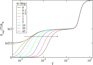
Figure 2: (Color online) The impurity contribution to the electron entropy as a function of the temperature for different values of the parameter $\alpha$ which quantifies the ratio of Majorana hopping rates. The model parameters are $U=0.2$, $\Gamma_{\uparrow}=\Gamma_{\downarrow}=0.01$ (for the $t_{1}=t_{2}$ limit), and $\epsilon+U/2=0$. The arrow indicates the direction of increasing $\alpha$.

In Fig. 3 we show charge fluctuations and the low-temperature scale $T_{L}$ of the problem as a function of $\alpha$ (for small $\alpha$, there are actually two different low-temperature scales, one associated with the Kondo screening and the other with the cross-over from the NFL to the Fermi-liquid (FL) state; the results for $T_{L}$ are actually meaningful only for large $\alpha>5^{\circ}$, where they roughly correspond to the Kondo temperature of the conventional Kondo screening). We see that reducing $\alpha$ leads to a small reduction of charge fluctuations (by approximately $7\%$); this corresponds to the gradual freezing-out of the fluctuations of one of the Majorana modes. The low-temperature scale of the problem decreases accordingly. This behavior is similar to that found in the ferromagnetic Kondo problem, where with the increasing polarization $P$ the charge fluctuations of both spin species are reduced [even though the average hybridization $(\Gamma_{\uparrow}+\Gamma_{\downarrow})/2$ remains constant, thus the hybridization of one spin species decreases while that of the other actually increases] and the Kondo temperature is exponentially lowered.

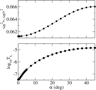
Figure 3: a) Charge fluctuations as a function of the parameter $\alpha$. b) The low-temperature scale of the problem, defined as $S(T_{L})=3\ln 4/4$. In the regime where the regular Kondo effect scaling is observed (roughly $\alpha>5^{\circ}$), $T_{L}$ approximately corresponds to the Kondo temperature $T_{K}$.

The Kondo temperature in the NFL regime ($t_{2}=0$) can be tuned by changing either of the two hybridization parameters, $\Gamma_{\uparrow}$ (that is, the coupling to the TS) or $\Gamma_{\downarrow}$ (the coupling to the probe leads). In both cases the dependence is exponential, see Fig. 4. We reiterate in passing that $\Gamma_{\uparrow}$ and $\Gamma_{\downarrow}$ by no means have to be equal for the two-channel Kondo effect to emerge.

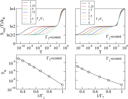
Figure 4: (Color online) The temperature scales as a function of the hybridization with the Majorana mode ($\Gamma_{\uparrow}$) and the measurement leads ($\Gamma_{\downarrow}$). In each case one of the hybridization parameters is held fixed at a value of $\Gamma_{\sigma}=0.01$, while the other is varied. $U=0.2$, $\epsilon_{d}=-U/2$.

III.2 Transport properties

In Fig. 5 we plot one of the main results of this work, the temperature dependence of the linear conductance as measured between the probe source and drain electrodes. The subfigures b,c,d show the results of a fit using an empirical function Goldhaber-Gordon et al. (1998); Parks et al. (2010)

$$G(T)=G_{0}\left[1+(2^{1/s}-1)(T/T_{K})^{p}\right]^{-s},$$ (20)

where $T_{K}$ is defined as $G(T_{K})=G(0)/2$, $p$ describes the exponent of the asymptotic behavior for small $T$ (Fermi liquid behavior corresponds to a $T^{2}$ finite-temperature correction, while for the two-channel Kondo model NFL fixed-point one expects a linear finite-temperature correction), while the parameter $s$ controls the shape of the cross-over part of the curve. We find that the parameter $T_{K}$ varies similarly as the low-temperature scale $T_{L}$ discussed previously. The shape parameter $s$ is at first decreasing, but in the low-$\alpha$ regime where the two-stage behavior starts to emerge (roughly $\alpha<5^{\circ}$) the conductance curves start to strongly reflect the non-Fermi-liquid behavior at low temperature scales. This is most strikingly visible in the behavior of the exponent parameter $p$ which rapidly decreases towards the expected limiting value of $p=1$. It is interesting to note that in the case of regular Anderson impurity model (i.e., for $\alpha=45^{\circ}$), the best fit is not obtained for the standard values $p=2$, $s=0.22$, but rather for $p\approx 1.8$, $s\approx 0.25$. This is due to the fact that the true $T^{2}$ behavior only emerges asymptotically for $T\ll T_{K}$, where the conductance is very close to the unitary limit, while in the cross-over regime a better description is obtained with an effective exponent different from 2. This is an important message for the experimentalists: a deviation of the extracted parameter $p$ from the value of 2 does not immediately imply non-Fermi-liquid properties of the system at low temperatures, especially if the fit is performed in the cross-over region. An extracted value approaching $p=1$ would, however, constitute a “smoking gun” that the system is near the two-channel Kondo model fixed point. Since the transport curves are universal, the proposed transport experiment would thus consist of measuring the conductance across one or two decades of temperatures (around and below $T_{K}$, for example) and fitting with the $G(T)$ curves. It is not necessary to go to very low temperatures ($T\ll T_{K}$) and try to extract the $T^{2}$ or $T$ scaling behavior; even on the scale of $T\sim T_{K}$ the universal $G(T)$ in both cases are sufficiently different that one should be able to distinguish the two situations (a comparison between the measured $G(T)$ curves and the NRG calculations, for example, shows good agreement and has been used to distinguish between the Kondo and the mixed-valence regimes Goldhaber-Gordon et al. (1998), or between the Kondo effects with different impurity spins Parks et al. (2010)).

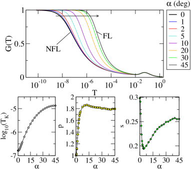
Figure 5: (Color online) a) Temperature dependence of the conductance through the quantum dot for different values of $\alpha$. The arrow indicates the direction of increasing $\alpha$. b,c,d) The variation of the fit parameters $T_{K}$, $p$, and $s$ as a function of $\alpha$.

Finally, we must address the role of the gate voltage and the magnetic field. Both types of operators are relevant (in the renormalization group sense), since in the language of the Majorana fermions they correspond to various coupling terms such as $d^{\dagger}_{\sigma}d_{\sigma}=-i\xi_{1\sigma}\xi_{2\sigma}$ where $\xi_{i\sigma}$ are the Majorana modes of the impurity. Strictly speaking, the non-Fermi-liquid fixed point is only stable at the particle-hole symmetric point ($\epsilon+U/2=0$) and for zero external magnetic field ($B=0$), thus the system needs to be tuned appropriately to observe the two-channel Kondo effect. Note, however, that we have assumed particle-hole symmetric flat bands. In general, the bands will have some non-trivial density of states. In this case, the NFL fixed point will be shifted away from the $\epsilon+U/2=0$, $B=0$ point and the condition for observing the 2CK effect is such that the induced magnetic and electric field in the quantum dot are compensated. This is similar to the physics of the Kondo effect in the presence of ferromagnetic leads Martinek et al. (2003a, b); Choi et al. (2004); Pasupathy et al. (2004).

It is worth noting that the two-channel Kondo effect may, in principle at least, be easier to achieve in this system than in the semiconductor quantum dot implementation of Ref. Potok et al., 2007. In the latter system, the NFL fixed point is achieved by using a larger (but interacting) quantum dot to effectively play the role of the second channel (inter-channel particle exchange is dynamically prohibited by the penalty of the charging energy); this then requires a subtle tuning to obtain equal coupling to both channels, $J_{1}=J_{2}$. In the proposed system, there are always only three Majorana channels, and one solely needs to tune the quantum dot parameters such that one of the local Majorana modes decouples. (In this respect the problem is similar to the case of a QD coupled to the edge states of the FQHE Fiete et al. (2008), where one also needs to tune solely the QD parameters. The required channel symmetry is automatically present.)

III.3 Magnetic field effects

The system may also be probed at constant temperature by applying an external magnetic field (which is assumed to couple only to the dot spin without perturbing other parts of the system). In the standard Kondo effect, the magnetic field reduces the linear conductance at $T=0$ quadratically for small $B$ Costi (2000); Hewson (1993). In fact, one may use a fitting function similar to Eq. (20):

$$G(T=0,B)=G_{0}\left[1+(2^{1/s^{\prime}}-1)(B/T_{K})^{p^{\prime}}\right]^{-s^{\prime}},$$ (21)

where $B$ is expressed in temperature units $(g\mu_{B}/k_{B}$). When a fit is performed for a FL regime over an interval of magnetic fields from $B=0$ to $B=T_{K}$, one obtains for the exponent $p^{\prime}=2$ and for the shape parameter $s^{\prime}=0.5$. Performing the same calculation for our system in the NFL regime, we obtain, instead, the exponent $p^{\prime}=1.3$ and the shape parameter $s^{\prime}=0.36$. More extensive set of results for the conductance at finite temperature and magnetic field are shown in Fig. 6. The results in the FL and NFL regimes are characteristically different and allow for an additional measurement approach.

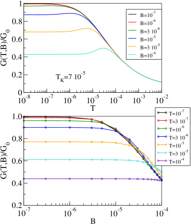
Figure 6: (Color online) Temperature and magnetic-field dependence of the conductance through the quantum dot. Model parameters are $U=0.2$, $\epsilon=-U/2$, $\Gamma_{\uparrow}=0.03$, and $\Gamma_{\downarrow}=0.01$.

IV Conclusion

It was shown that if a quantum impurity described as a single interacting level is coupled to three independent Majorana channels, but is decoupled from the fourth, a non-Fermi-liquid state emerges which can be probed by performing linear conductance measurements. By tuning the system parameters (in particular the gate voltage) the non-Fermi-liquid regime can be obtained even in situations which do not have the full O(3) symmetry between the three Majorana channels. The experimental realization of the predicted effect could make use of two QAH systems to provide fully spin-polarized complex fermions, and one TSC system to provide the Majorana fermions of the opposite spin. The experimental challenge thus consists – in the first place – in actually creating the QAH and TSC systems, and in establishing the electrical contacts between the quantum dot and these systems. The non-Fermi-liquid state should then naturally emerge and it should be rather robust (as robust as the edge states themselves). Further complications might arise from the interactions between the electrons in the one-dimension channels, since they might drive the system to a different fixed point.

Appendix A Majorana resonant-level model

For reference purposes (and for testing the numerical method) we now solve exactly the resonant-level model with different couplings to the two Majorana modes of a single-channel continuum. The spin index plays no role in a non-interacting model, thus we omit it in writing. The Hamiltonian is composed of the following terms:

$$\begin{split}H_{0}&=\epsilon n_{\sigma},\\ H_{1}&=\sum_{k}\epsilon_{k}c^{\dagger}_{k}c_{k},\\ H_{2}&=\sum_{k}\left(Vc^{\dagger}_{k}d+Ac^{\dagger}_{k}d^{\dagger}+\text{H.c.}\right).\end{split}$$ (22)

We assume that the hopping coefficients $V$ and $A$ do not depend on $k$, and for simplicity we take them to be real. We will use the notation $\langle\langle A;B\rangle\rangle_{z}$ for a correlator between the operators $A$ and $B$, and at the end the argument $z$ will be chosen as $z=\omega+i\delta$ to obtain the retarded Green’s functions ($\delta\to 0$). We are particularly interested in the Green’s function $G(\omega)=\langle\langle d;d^{\dagger}\rangle\rangle_{\omega+i\delta}$ which gives the spectral function as $A(\omega)=(-1/\pi)\mathrm{Im}G(\omega)$. We use the equation of motion method:

$$z\langle\langle A;B\rangle\rangle_{z}=\langle[A,B]_{\eta}\rangle-\langle\langle A;[B,H]_{-}\rangle\rangle_{z},$$ (23)

where $\eta=+$ (anticommutator) if $A$ and $B$ are both fermionic operators, and $\eta=-$ (commutator) in all other cases.

We introduce the notation $g=\langle\langle d;d^{\dagger}\rangle\rangle_{z}$ and $h=\langle\langle d;d\rangle\rangle$, as well as $g_{k}=\langle\langle d;c_{k}^{\dagger}\rangle\rangle$ and $h_{k}=\langle\langle d;c_{k}\rangle\rangle$. The equations of motion then give

$$\begin{split}(z-\epsilon)g&=1+V\sum_{k}g_{k}-A\sum_{k}h_{k},\\ (z-\epsilon_{k})g_{k}&=Vg+Ah,\\ (z+\epsilon)h&=-V\sum_{k}h_{k}+A\sum_{k}g_{k},\\ (z+\epsilon_{k})h_{k}&=-Ag-Vh.\end{split}$$ (24)

We introduce $\gamma_{1}(z)=\sum_{k}1/(z-\epsilon_{k})$ and $\gamma_{2}(z)=\sum_{k}1/(z+\epsilon_{k})$, whose imaginary parts for argument $z=\omega+i\delta$ are proportional to the density of states in the lead, $\rho(\omega)$. For a particle-hole symmetric band, $\gamma_{1}$ and $\gamma_{2}$ are fully equivalent. Expressing $g_{k}$ and $h_{k}$ in terms of $g$ and $h$, inserting them in the equations of motion for $g$ and $h$, then solving the resulting equations for $g$, we obtain

$$g=\frac{\epsilon+z-(A^{2}\gamma_{1}+V^{2}\gamma_{2})}{(c\gamma_{1}-\epsilon)(c\gamma_{2}+\epsilon)-d(\gamma_{1}+\gamma_{2})z+z^{2}},$$ (25)

where $c=A^{2}-V^{2}$ and $d=A^{2}+V^{2}$. In the wide-band limit, $\gamma_{1,2}\to-i\pi\rho$, where $\rho$ is the constant density of states. The spectral function is then

$$A(\omega)\approx\frac{1}{\pi}\frac{\pi\rho d\left[(\pi\rho c)^{2}-(\omega+\epsilon)^{2}\right]}{[(\pi\rho c)^{2}+\epsilon^{2}]^{2}+2[(\pi\rho)^{2}(A^{4}+6A^{2}V^{2}+V^{4})-\epsilon^{2}]\omega^{2}+\omega^{4}}.$$ (26)

In the particle-hole symmetric case ($\epsilon=0$), the half-width at half-maximum of the spectral function is

$$\Gamma=\pi\rho\left[\left(A^{8}-4A^{6}V^{2}+70A^{4}V^{4}-4A^{2}V^{6}+V^{8}\right)^{1/2}-8A^{2}V^{2}\right]^{1/2}.$$ (27)

For $A=0$, this expression reduces to the expected result $\Gamma=\pi\rho V^{2}$. In the $V=0$ limit, the result is $\Gamma=\pi\rho A^{2}$. For $|A|\to|V|$ the width of the resonance goes to zero and a delta peak emerges in the spectral function at $\omega=0$, see also Ref. Bradley et al., 1999. This corresponds to the case of a fully decoupled Majorana mode. Strictly speaking, the system is then in a NFL state with $\ln 2/2$ residual entropy (per spin). The delta peak carries half the spectral weight and there is a broader background peak associated with the hybridized Majorana partner of the decoupled mode; this broad spectral peak carries the remaining half of the spectral weight.

If the problem is not particle-hole symmetric ($\epsilon\neq 0$) the two Majorana modes remain coupled through the charge term (since $d^{\dagger}d=-i\eta_{1}\eta_{2}$). In this case there can be no decoupled Majorana mode and at zero temperature the system is in a FL state for all values of $A$ and $V$. As $|A|\to|V|$, the spectral function will have a maximum at $\omega\approx\epsilon$ (with a shift of the order of the spectral peak width $\Gamma$) and will touch zero exactly at $\omega=-\epsilon$.

The anomalous Green’s function $h(z)=\langle\langle d;d\rangle\rangle_{z}$ is

$$h=\frac{AV(\gamma_{1}+\gamma_{2})}{(c\gamma_{1}-\epsilon)(c\gamma_{2}-\epsilon)-d(\gamma_{1}+\gamma_{2})z+z^{2}}.$$ (28)

It is proportional to $A$, thus it vanishes in the absence of the anomalous hybridization. In the wide-band limit, the anomalous spectral function $B(\omega)=(-1/\pi)\mathrm{Im}h(\omega+i\delta)$ is

$$B(\omega)\approx\frac{-1}{\pi}\frac{2\pi\rho AV\left((\pi\rho c)^{2}+(\epsilon-\omega)(\epsilon+\omega)\right)}{[(\pi\rho c)^{2}+\epsilon^{2}]^{2}+2[(\pi\rho)^{2}(A^{4}+6A^{2}V^{2}+V^{4})-\epsilon^{2}]\omega^{2}+\omega^{4}}.$$ (29)

In the particle-hole symmetric case ($\epsilon=0$) this spectral function has an inverted (negative) peak at $\omega=0$ superimposed on a broader positive resonance. In the $|A|\to|V|$ limit, the inverted peak narrows down until it becomes a delta peak. This feature thus corresponds to the decoupled Majorana mode, while the positive broad resonance corresponds to its Majorana partner state.

For $\epsilon\neq 0$, the spectral function $B(\omega)$ goes through zero always at $\omega=\pm\epsilon$, i.e., $|\epsilon|$ sets the scale of the inverted spectral peak. As $|A|\to|V|$ only the weight of this peak saturates, while the width remains roughly constant, since the Majorana mode does not decouple.