Polytropic configurations with non-zero cosmological constant

Abstract

We solve the equation of the equilibrium of the gravitating body, with a polytropic equation of state of the matter $P=K\rho^{\gamma}$, with $\gamma=1+1/n$, in the frame of the Newtonian gravity, with non-zero cosmological constant $\Lambda$. We consider the cases with $n=1,\,\,1.5,\,\,3$ and construct series of solutions with a fixed value of $\Lambda$. For each value of $n$, the non-dimensional equation of the static equilibrium has a family of solutions, instead of the unique solution of the Lane-Emden equation at $\Lambda=0$. The equilibrium state exists only for central densities $\rho_{0}$ larger than the critical value $\rho_{c}$. There are no static solutions at $\rho_{0}<\rho_{c}$. We investigate the stability of equilibrium bodies in presence of nonzero $\Lambda$, and show that dark energy decease the dynamic stability of the configuration. We apply our results for analyzing the properties of equilibrium states for cluster of galaxies in the present universe with non-zero $\Lambda$.

1 Introduction

Detailed analysis of the observations of distant SN Ia (Riess et al., 1998; Perlmutter et al., 1999) and of the spectrum of fluctuations of the cosmic microwave background radiation (CMB), see e.g. Spergel et al. (2003), Tegmark et al. (2004), have lead to conclusion that the term, representing “dark energy” contains about 70% of the average energy density in the present universe and its properties are very close (identical) with the properties of the Einstein cosmological $\Lambda$ term. This value of the cosmological constant was anticipated by Kofman & Starobinsky (1985), basing on the analysis of the existing upper limits for the microwave background anisotropy, see also Eke et al. (1996). In papers of Chernin (see reviews 2001 and 2008) the question was raised about a possible influence of the existence of the cosmological constant on the properties of the Hubble flow in the local galaxy cluster at close vicinity of our Galaxy. Basing on the observations of Karachentsev et al. (2006), it was concluded by Chernin (2001, 2008) that the presence of the the dark energy (DE) is responsible for the formation of this Hubble flow. This conclusion was criticized by Lukash & Rubakov (2008).

The importance of the DE for the structure of the local galaxy cluster (LC) depends on the level of the influence of DE on the dynamic properties. In particular, it is necessary to check, if the LC may exist in the equilibrium state, at present values of DE density, and the LC densities of matter, consisting of the baryonic and dark matter (BM and DM).

Here, we construct, in Newtonian approximation, exact equilibrium configurations of the selfgravitating objects in presence of DE. We consider a polytropic equation of state, having in mind, that very extended configurations, like LC, where the dark matter have not reached the state of a full thermodynamic equilibrium, and effective temperature could be not a constant over the cluster. In presence of DE ($\Lambda$) the polytropic configurations are represented by a family of configurations, instead of the single model for each polytropic index $n$. The additional parameter $\beta$ represents the ratio of the density of DE to the matter central density of the configuration. For values of $n=1,\,\,1.5,\,\,3$, corresponding to the polytropic powers $\gamma=2,\,\,5/3,\,\,4/3$, we find the limiting values of $\beta_{c}$, so that at $\beta>\beta_{c}$ there are no equilibrium configurations and only expanding cluster, may be with a Hubble flow, may exist. We apply these results to the LC using the observational data and different suggestions, connected with DM distribution. Note that the structure of the isothermal configurations in a box, in presence of DE was investigated by de Vega & Siebert (2005): in this paper the authors were interested in the problem of thermodynamic stability of such configurations, following the works of Antonov (1962) and Lynden-Bell & Wood (1968). We have derived a virial theorem for the equilibrium configurations in presence of DE, and investigate an influence of the DE on the dynamic stability of the equilibrium configurations, using an approximate energetic method. It is shown that DE produce a destabilizing effect, contrary to the stabilizing influence of the cold dark matter (McLaughlin & Fuller, 1996).

2 Main equations

Let us consider spherically symmetric equilibrium configuration in Newtonian gravity, in presence of DE, represented by the cosmological constant $\Lambda$. In this case, the gravitational force $F_{g}$ which a unit mass undergoes in a spherically symmetric body is given by the formula (Chandrasekhar, 1939)

$$F_{g}=-\frac{Gm}{r^{2}}+\frac{\Lambda r}{3},$$ (1)

where $m$ is the mass of the matter inside the radius $r$, which is connected with the matter density $\rho$ by the continuity equation

$$\frac{dm}{dr}=4\pi\rho r^{2}.$$ (2)

The density of DE $\rho_{v}$ is connected with $\Lambda$ as

$$\rho_{v}=\frac{\Lambda}{8\pi G}.$$ (3)

Then, the equilibrium equation of the selfgravitating body is given by

$$\frac{1}{\rho}\frac{dP}{dr}=-\frac{Gm}{r^{2}}+\frac{\Lambda r}{3}.$$ (4)

Now, let us consider a polytropic equation of state

$$P=K\rho^{\gamma},\quad{\rm with}\quad\gamma=1+\frac{1}{n}.$$ (5)

By introducing the nondimensional polytropic variables $\xi$ and $\theta_{n}$ so that (Chandrasekhar, 1939)

$$r=\alpha\xi\quad{\rm and}\quad\rho=\rho_{0}\theta_{n}^{n},$$ (6)

we obtain, from (2) and (4), the equation describing the structure of the polytropic configuration in presence of the DE as

$$\frac{1}{\xi^{2}}\frac{d}{d\xi}\left(\xi^{2}\frac{d\theta_{n}}{d\xi}\right)=-\theta_{n}^{n}+\beta.$$ (7)

Here $P$ is the pressure and $\rho_{0}$ is the matter central density, $\alpha$ is the characteristic radius given by

$$\alpha^{2}=\frac{(n+1)K}{4\pi G}\rho_{0}^{\frac{1}{n}-1},$$ (8)

while $\beta={\Lambda}/{4\pi G\rho_{0}}={2\rho_{v}}/{\rho_{0}}$ represents the ratio of the DE density to the central density of the configuration. At $\beta=0$ we obtain from (7) the well known Lane-Emden equation (Chandrasekhar, 1939).

Note, that the generalization of Lane-Emden equation in presence of $\Lambda$ was first obtained by Balaguera-Antolínez et al. (2007).

3 The virial theorem

Let us find the relations between gravitational $\varepsilon_{g}$ and thermal $\varepsilon_{th}$ energies, and the energy $\varepsilon_{\Lambda}$, of the interaction of the body with DE. The gravitational energy of the selfgravitation is written as (Landau & Lifshitz, 1980)

$$\varepsilon_{g}=-G\int_{0}^{M}\frac{mdm}{r},\quad m=4\pi\int_{0}^{r}\rho{r^{\prime}}^{2}dr^{\prime}=-\frac{r^{2}}{G}\left(\frac{1}{\rho}\frac{dP}{dr}-\frac{\Lambda r}{3}\right),\quad M=m(R).$$ (9)

Here $m$ is written using the equilibrium equation (4). For the adiabatic stars with a polytropic equation of state we have the relations

$$\rho E=nP,\quad I=E+\frac{P}{\rho}=\frac{n+1}{n}E,$$ (10)

where $E$ and $I$ are thermal energy and enthalpy per mass unit. After some transformations, similar to ones made by Landau & Lifshitz (1980), we obtain the following relations between the energies

$$\varepsilon_{g}=-\frac{3}{n}\varepsilon_{th}+2\varepsilon_{\Lambda},\qquad\varepsilon_{th}=-\frac{n}{3}\varepsilon_{g}+\frac{2n}{3}\varepsilon_{\Lambda},$$ (11)

$$\varepsilon_{tot}=\varepsilon_{th}+\varepsilon_{g}+\varepsilon_{\Lambda}=\frac{3-n}{3}\varepsilon_{g}+\frac{2n+3}{3}\varepsilon_{\Lambda}=\frac{n-3}{n}\varepsilon_{th}+3\varepsilon_{\Lambda}.$$ (12)

where $\varepsilon_{\Lambda}=-\frac{4\pi G\rho_{v}}{3}\int_{0}^{M}r^{2}dm=-\frac{\Lambda}{6}\int_{0}^{M}r^{2}dm$ is defined below in (40) and the additive constant in the energy definition of $\varepsilon_{\Lambda}$ is chosen so that $\varepsilon_{\Lambda}=0$ at $\Lambda=0$ and $M=0$, being $\varepsilon_{th}=\int_{0}^{M}E\,dm$. Now, let us make an additional transformation of the expression for $\varepsilon_{g}$. Then, by partial integration, we obtain

$$\varepsilon_{g}=-G\int_{0}^{M}\frac{mdm}{r}=-\frac{GM^{2}}{2R}-\frac{G}{2}\int_{0}^{R}\frac{m^{2}}{r^{2}}dr.$$ (13)

We can transform the last integral by using (9), (10) and making partial integrations. We have

$$\frac{G}{2}\int_{0}^{R}\frac{m^{2}}{r^{2}}dr=-\frac{1}{2}\int_{0}^{R}r^{2}\left(\frac{1}{\rho}\frac{dP}{dr}-\frac{\Lambda r}{3}\right)\frac{m}{r^{2}}dr=-\frac{1}{2}\int_{0}^{R}\frac{m}{\rho}\frac{dP}{dr}dr+\frac{\Lambda}{6}\int_{0}^{R}mr\,dr$$

$$=\frac{1}{2}\int_{0}^{M}I\,dm+\frac{\Lambda}{12}MR^{2}-\frac{\Lambda}{12}\int_{0}^{M}r^{2}\,dm=\frac{n+1}{2n}\varepsilon_{th}+\frac{\Lambda}{12}MR^{2}+\frac{\varepsilon_{\Lambda}}{2}.$$ (14)

Then, by using (11), (14), we obtain from (13) the following relations

$$\varepsilon_{g}=-\frac{3}{5-n}\frac{GM^{2}}{R}-\frac{\Lambda}{2(5-n)}MR^{2}-\frac{2n+5}{5-n}\varepsilon_{\Lambda},$$ (15)

$$\varepsilon_{th}=\frac{n}{5-n}\frac{GM^{2}}{R}+\frac{n\Lambda}{6(5-n)}MR^{2}+\frac{5n}{5-n}\varepsilon_{\Lambda}.$$ (16)

Finally, by inserting (16) in (12), we get

$$\varepsilon_{tot}=\frac{n-3}{5-n}\frac{GM^{2}}{R}+\frac{(n-3)\Lambda}{6(5-n)}MR^{2}+\frac{2n}{5-n}\varepsilon_{\Lambda}.$$ (17)

We can calculate $\varepsilon_{tot}$ for some particular cases. For $n=3,\,\,1,\,\,{\rm and}\,\,0$ we have, respectively.

$$\varepsilon_{tot}=3\varepsilon_{\Lambda},\quad\varepsilon_{tot}=-\frac{1}{2}\frac{GM^{2}}{R}-\frac{1}{12}\Lambda MR^{2}+\frac{1}{2}\varepsilon_{\Lambda},\quad\varepsilon_{tot}=-\frac{3}{5}\frac{GM^{2}}{R}-\frac{1}{10}\Lambda MR^{2},$$ (18)

The Lane-Emden model with $n=5$, has an analytical solution with finite mass $M$, finite values of the energies and infinite radius $R$, so that must be $(5-n)R\,\rightarrow\,{\rm const}$, if $n\rightarrow 5$. In presence of DE the finiteness of values of all types of energies require that

$$(5-n)R\,\rightarrow\,{\rm const}\quad{\rm and}\quad\varepsilon_{\Lambda}\,\rightarrow\,-\frac{\Lambda}{30}MR^{2},\,\,{\rm if}\,\,\,n\rightarrow 5.$$ (19)

The Lane-Emden solution (without DE) at $n=3$ has the zero total energy, with a given finite radius and corresponds to a neutral equilibrium. So, the knowledge of the total energy of the configuration permits to find the boundary between dynamically stable ($n<3$, $\varepsilon_{tot}<0$) and unstable ($n>3$, $\varepsilon_{tot}>0$) configurations. In our case the virial theorem does not permit to do it, because the value of $\varepsilon_{\Lambda}$ is not properly defined, while the presence of DE in the whole space does not permit to chose, in a simple way, a universal additive constant of the energy. Therefore, in spite of the result from (18), where $\varepsilon_{tot}=3\varepsilon_{\Lambda}<0$ at $n=3$, in accordance to the stability analysis made in section 4.3, the polytropic solution at $n=3$ in presence of DE becomes unstable.

The virial theorem in presence of $\Lambda$ was investigated by Balaguera-Antolínez et al. (2007). The final result in this paper was presented in the form of integrals, instead of simple algebraic relations obtained above.

4 Equilibrium solutions

4.1 The case n=1

At $n=1$ the equation (7) is linear and has an analytic solution. Following Chandrasekhar (1939), let us introduce a new variable $\chi=\xi\theta_{1}$. After the substitution the equation (7) is transformed into

$$\frac{d^{2}\chi}{d\xi^{2}}=-\chi+\xi\beta.$$ (20)

At $\beta=0$ we have a well known analytic polytropic solution (Chandrasekhar, 1939)

$$\theta_{1}=\frac{\sin\xi}{\xi},$$ (21)

satisfying the boundary conditions in the center $\theta_{1}(0)=1$, $\theta_{1}^{\prime}(0)=0$. At nonzero $\beta$, the solution satisfying the boundary conditions in the center is written as

$$\theta_{1}=(1-\beta)\frac{\sin\xi}{\xi}+\beta.$$ (22)

The radius of the configuration is defined by the first zero of the solution (21), or (22). For the Lane-Emden solution (21) the outer radius corresponds to $\xi_{out}=\pi$ and, for the solution of (22) with DE, the radius of the configuration is determined by the transcendental equation

$$(1-\beta)\frac{\sin\xi_{out}}{\xi_{out}}+\beta=0.$$ (23)

This equation has real solutions only at $\beta<\beta_{c}$, so that at the outer boundary not only $\theta_{1}=0$, but also $\theta_{1}^{\prime}=0$ for $\beta=\beta_{c}$. It follows from (22)

$$\theta_{1}^{\prime}=(1-\beta)\left(\frac{\cos\xi}{\xi}-\frac{\sin\xi}{\xi^{2}}\right).$$ (24)

therefore the parameters $\beta_{c}$ and $\xi_{out,c}$ of the limiting equilibrium solution in presence of DE are determined by the algebraic equations

$$(1-\beta_{c})\frac{\sin\xi_{out,c}}{\xi_{out,c}}+\beta_{c}=0,\quad\tan\xi_{out,c}=\xi_{out,c},\quad\pi\,<\,\xi_{out,c}\,<\,\frac{3\pi}{2}.$$ (25)

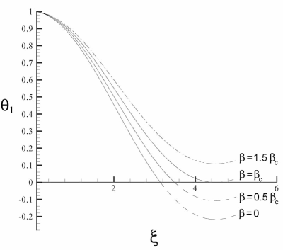
Figure 1: The density distribution for configurations at $n=1$ with $\beta=0,\,\,\beta=0.5\beta_{c},\,\,\beta=\beta_{c}$. The curves are marked with the values of $\beta$. The nonphysical solution at $\beta=1.5\beta_{c}$, which has not an outer boundary, is given by the dash-dot line. The nonphysical parts of the solutions at $\beta\leq\beta_{c}$, behind the outer boundary, are given by the dash lines. The solutions, at large $\xi$, asymptotically approach the horizontal line $\theta_{1}=\beta$.

The density distribution for the equilibrium configurations with values $\beta=0,\,\,\beta=0.5\beta_{c},\,\,\beta=\beta_{c}$ is shown in Fig.1. The nonphysical solution at $\beta=1.5\beta_{c}$, which has not an outer boundary, is given by the dash-dot line. The nonphysical parts of the solutions at $\beta\leq\beta_{c}$, behind the outer boundary, are given by dash lines. At large $\xi$, these solutions asymptotically approach the horizontal line $\theta_{1}=\beta$. Numerical solutions of equations (25) and (23) give $\beta_{c}=0.178$ and $\xi_{out}=\pi,\,\,3.490,\,\,4.493$, for $\beta=0,\,\,\beta=0.5\beta_{c}=0.089,\,\,\beta=\beta_{c}=0.178$, respectively.

4.2 Some general relations

The equilibrium mass $M_{n}$ for a generic polytropic configuration which is solution of the Lane-Emden equation is written as

$$M_{n}=4\pi\int_{0}^{R}\rho r^{2}dr=4\pi\left[\frac{(n+1)K}{4\pi G}\right]^{3/2}\rho_{0}^{\frac{3}{2n}-\frac{1}{2}}\int_{0}^{\xi_{out}}\theta_{n}^{n}\xi^{2}d\xi.$$ (26)

Using equation (7), the integral in the right site may be calculated by partial integration, what gives the following relation for the mass of the configuration

$$M_{n}=4\pi\left[\frac{(n+1)K}{4\pi G}\right]^{3/2}\rho_{0}^{\frac{3}{2n}-\frac{1}{2}}\left[-\xi_{out}^{2}\left(\frac{d\theta_{n}}{d\xi}\right)_{out}+\frac{\beta\xi_{out}^{3}}{3}\right].$$ (27)

Reminding (8), we can write the expression for the mass in the form

$$M_{n}=4\pi\rho_{0}\alpha^{3}\left[-\xi_{out}^{2}\left(\frac{d\theta_{n}}{d\xi}\right)_{out}+\frac{\beta\xi_{out}^{3}}{3}\right].$$ (28)

Let us note, that here $\theta_{n}(\xi)$ is not a unique function, but it depends on the parameter $\beta$, according to (7). For the limiting configuration, with $\beta=\beta_{c}$, we have on the outer boundary $\xi_{out}$

$$\theta_{n}(\xi_{out})=0,\quad\frac{d\theta_{n}}{d\xi}|_{\xi_{out}}=0.$$ (29)

Therefore the mass $M_{n,lim}$ of the limiting configuration, with account of (6), is written as

$$M_{n,lim}=4\pi\rho_{0c}\alpha^{3}\frac{\beta_{c}\xi_{out}^{3}}{3}=\frac{4\pi}{3}r_{out}{{}^{3}}\beta_{c}\rho_{0c}=\frac{4\pi}{3}r_{out}{{}^{3}}\bar{\rho}_{c},$$ (30)

so that the limiting value $\beta_{c}$ is exactly equal to the ratio of the average matter density $\bar{\rho}_{c}$ of the limiting configuration, to its central density $\rho_{0c}$

$$\beta_{c}=\frac{\bar{\rho}_{c}}{\rho_{0c}}.$$ (31)

For the Lane-Emden solution (with $\beta=0$) we have $\rho_{0}/\bar{\rho}=3.290,\,\,5.99,\,\,54.18$ for $n=1,\,\,1.5,\,\,3$, respectively. Let us consider the curve $M(\rho_{0})$ for a constant DE density $\rho_{v}=\Lambda/8\pi G$. For plotting this curve in the nondimensional form, we introduce the characteristic density $\rho_{ch}$ and write the expression for the mass in the form

$$M_{n}=4\pi\left[\frac{(n+1)K}{4\pi G}\right]^{3/2}\rho_{ch}^{\frac{3}{2n}-\frac{1}{2}}\hat{\rho}^{\frac{3}{2n}-\frac{1}{2}}\left[-\xi_{out}^{2}\left(\frac{d\theta_{n}}{d\xi}\right)_{out}+\frac{\beta\xi_{out}^{3}}{3}\right],$$ (32)

where $\hat{\rho}_{0}=\rho_{0}/\rho_{ch}$ is the nondimensional central density of the configuration. We introduce also the nondimensional mass of the confuguration ${\hat{M}_{n}}$ as

$$M_{n}=4\pi\left[\frac{(n+1)K}{4\pi G}\right]^{3/2}\rho_{ch}^{\frac{3}{2n}-\frac{1}{2}}{\hat{M}_{n}},\quad{\hat{M}_{n}}=\hat{\rho}_{0}^{\frac{3}{2n}-\frac{1}{2}}\left[-\xi_{out}^{2}\left(\frac{d\theta_{n}}{d\xi}\right)_{out}+\frac{\beta\xi_{out}^{3}}{3}\right].$$ (33)

Now we can plot the nondimensional curve ${\hat{M}_{n}}({\hat{\rho}_{0}})$, at constant $\rho_{v}=\beta\rho_{0}/2$ (from the definition of $\beta$). It is convenient to construct the curve starting from the model with $\hat{\rho}_{0}=1$ and $\beta\ll 1$, very close to the Lane-Emden solution, and than following the sequence by decreasing the central density $\hat{\rho}_{0}$ with taking $\beta\propto 1/\hat{\rho}_{0}$ (being constant $\rho_{v}$) until the value $\beta=\beta_{c}$. For $n=1$, using (24), we have

$$\hat{M}_{1}=\hat{\rho}_{0}\left[(1-\beta)(\sin\xi_{out}-\xi_{out}\cos\xi_{out})+\frac{\beta\xi_{out}^{3}}{3}\right],\quad\hat{\rho}_{0}\beta=\beta_{in}\,=\,{\rm const}.$$ (34)

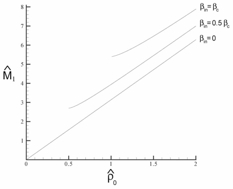
Figure 2: Nondimensional mass $\hat{M}_{1}$ of the equilibrium polytropic configurations at $n=1$ as a function of the nondimensional central density $\hat{\rho}_{0}$, for different values of $\beta_{in}$. The cosmological constant $\Lambda$ is the same along each curve. The curves at $\beta_{in}\neq 0$ are limited by the configuration with $\beta=\beta_{c}$.

The behavior of $\hat{M}_{1}(\hat{\rho}_{0})|_{\Lambda}$ (at constant $\rho_{v}$) is given in Fig.2 for different values of $\beta_{in}=0,\,\,\beta_{in}=0.5\beta_{c},\,\,\beta_{in}=\beta_{c}$, for which $\hat{M}_{1}=\pi,\,\,3.941,\,\,5.397$ at $\hat{\rho}_{0}=1$. We note that for $\beta_{in}=\beta_{c}$ there are equilibrium models only for $\hat{\rho}_{0}>1$.

4.3 The case n=3. Dynamic stability

The equilibrium equation for this case is

$$\frac{1}{\xi^{2}}\frac{d}{d\xi}\left(\xi^{2}\frac{d\theta_{3}}{d\xi}\right)=-\theta_{3}^{3}+\beta.$$ (35)

The mass of the configuration is given by

$$M_{3}=4\pi\left[\frac{K}{\pi G}\right]^{3/2}{\hat{M}_{3}},\quad{\hat{M}_{3}}=-\xi_{out}^{2}\left(\frac{d\theta_{3}}{d\xi}\right)_{out}+\frac{\beta\xi_{out}^{3}}{3}.$$ (36)

The Lane-Emden model ($\beta=0$) has a unique value of the mass, independent on the density (equilibrium configuration with neutral dynamical stability). At $\beta\neq 0$ the dependence on the density appears because the function $\theta_{3}$ is different for different values of $\beta$ and, along the curve $\hat{M}_{3}(\hat{\rho}_{0})|_{\Lambda}$, the value of $\beta$ is inversely proportional to $\hat{\rho}_{0}$ (like in the case $n=1$).

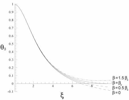
Figure 3: Same as in Fig.1, for $n=3$. The solutions asymptotically approach, at large $\xi$, the horizontal line $\theta_{3}=\beta^{1/3}$.

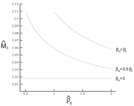
Figure 4: Same as in Fig.2, for $n=3$.

The density distribution for equilibrium configurations with $\beta=0,\,\,\beta=0.5\beta_{c},\,\,\beta=\beta_{c}$ is shown in Fig.3. The nonphysical solution at $\beta=1.5\beta_{c}$, which has not an outer boundary, is given by the dash-dot line. The nonphysical parts of the solutions at $\beta\leq\beta_{c}$, behind the outer boundary, are given by the dash lines. At large $\xi$, these solutions asymptotically approach the horizontal line $\theta_{3}=\beta^{1/3}$, with damping oscillations around this value. The numerical solution of the equation (35) gives $\beta_{c}=0.006$, $\xi_{out}=6.897,\,\,7.489,\,\,9.889$, for $\beta=0,\,\,\beta=0.5\beta_{c}=0.003,\,\,\beta=\beta_{c}=0.006$, respectively. In Fig.4 we show the behavior of $\hat{M}_{3}(\hat{\rho}_{0})|_{\Lambda}$, for different values of $\beta_{in}=0,\,\,\beta_{in}=0.5\beta_{c},\,\,\beta_{in}=\beta_{c}$, for which $\hat{M}_{3}=2.018,\,\,2.060,\,\,2.109$, at $\hat{\rho}_{0}=1$, respectively.

The behavior of $\hat{M}_{3}(\hat{\rho}_{0})|_{\Lambda}$ in Fig.4, showing a decreasing mass with the increase of the central density, corresponds, for an adiabatic index equal to the polytropic one, to dynamically unstable configurations, according to the static criterium of stability (Zel’dovich, 1963). When the vacuum influence is small, it is possible to investigate the stability of the adiabatic configuration by the approximate energetic method (Zeldovich & Novikov, 1966; Bisnovatyi-Kogan, 2001). For $n=3$, at $\rho_{0}\gg\rho_{v}$, the density in the configuration is distributed according to the Lane-Emden solution $\rho=\rho_{0}\,\theta_{3}^{3}(\xi)$. In this case we may investigate the stability to homologous perturbations, changing only the central density at fixed density distribution, given by the function $\theta_{3}$. Let us first calculate the newtonian gravitational energy of the configuration at presence of the cosmological constant (DE). For spherical configurations, the Poisson equation for the gravitational potential $\varphi_{*}$, in presence of DE is given by

$$\Delta\varphi_{*}=\frac{1}{r^{2}}\frac{d}{dr}\left(r^{2}\frac{d\varphi_{*}}{dr}\right)=4\pi G(\rho-2\rho_{v}),\quad\varphi_{*}=\varphi+\varphi_{\Lambda}.$$ (37)

The gravitational energy of a spherical body $\varepsilon_{g}$, connected with its selfgravity, is written as (Landau & Lifshitz, 1980)

$$\varepsilon_{g}=-G\int_{0}^{M}\frac{mdm}{r},\quad m=4\pi\int_{0}^{r}\rho r^{2}dr,\quad M=m(R),$$ (38)

where $R$ is the radius of body. Here, differently from the gravitational potential $\varphi$ where we have the normalization $\varphi=0$ at $r=\infty$, for $\varphi_{\Lambda}$ with uniform density $\rho_{v}$ this normalization is not possible. Then we can choose $\varphi_{\Lambda}=0$ at $r=0$ as the most convenient normalization. This choice, together using the equation (37), leads to the following expression

$$\varphi_{\Lambda}=-\frac{4\pi G\rho_{v}}{3}r^{2}.$$ (39)

Consequently, the gravitational energy $\varepsilon_{\Lambda}$, connected with the interaction of the matter with DE, is given by

$$\varepsilon_{\Lambda}=\int_{0}^{M}\varphi_{\Lambda}dm=-\frac{4\pi G\rho_{v}}{3}\int_{0}^{M}r^{2}dm.$$ (40)

In order to analyze the effects due to the presence of DE on the dynamical stability of spherical systems with a polytropic equation of state, it is necessary to consider configurations close to the polytropic (adiabatic) equilibrium solution at $n=3$ (and $\beta=0$), where the turning point of stability is expected. In this case, the presence of DE does not affect significantly the gravitational equilibrium because the nondimensional density profile of the configuration keeps constant during the adiabatic perturbation (homologous displacement), so that we can neglect the term depending on $\Lambda$ in the Lane-Emden equation and the nondimensional quantities $\xi_{out}$ and $\theta_{3}(\xi)$ of the unperturbed polytropic solution at $n=3$ can be used in calculating the gravitational energy $\varepsilon_{g}$ connected to the selgravity. Therefore, also the terms depending on $\Lambda$ which appear in the expression (15) of $\varepsilon_{g}$ can be deleted and the gravitational energy $\varepsilon_{*}$ becomes

$$\varepsilon_{*}=\varepsilon_{g}+\varepsilon_{\Lambda}=-G\int_{0}^{M}\frac{m\,dm}{r}-\frac{4\pi G\rho_{v}}{3}\int_{0}^{M}r^{2}dm=-\frac{3}{2}\frac{GM^{2}}{R}-\frac{\Lambda}{6}\int_{0}^{M}r^{2}dm,$$ (41)

where, taking into account the nondimensional variables (6), the energy $\varepsilon_{\Lambda}$ can be written as

$$\varepsilon_{\Lambda}=-\frac{\Lambda}{6}\int_{0}^{M}r^{2}dm=-\frac{2}{3}\pi\rho_{0}\alpha^{5}\Lambda\int_{0}^{\xi_{out}}\theta_{3}^{3}\xi^{4}d\xi.$$ (42)

Here, the last integral in (42) has been calculated by Bisnovatyi-Kogan (2001) so that

$$\int_{0}^{\xi_{out}}\theta_{3}^{3}\xi^{4}d\xi=10.85.$$ (43)

In the analysis of the dynamical stability, let us consider the total energy $\varepsilon$ of the configuration. Then, in addition to the Newtonian gravitational energy $\varepsilon_{g}$ and the energy $\varepsilon_{\Lambda}$, we must also take into account the contribution of the thermal energy $\varepsilon_{th}$, corresponding to a specific energy density $E$ (energy per unit mass), and we may include a small correction $\varepsilon_{GR}$ due to general relativity (Bisnovatyi-Kogan, 2001). We obtain

$$\varepsilon=\varepsilon_{th}+\varepsilon_{g}+\varepsilon_{\Lambda}+\varepsilon_{GR}=$$ (44)

$$=\int_{0}^{M}E\,dm-0.639GM^{5/3}\rho_{0}^{1/3}-0.104\Lambda M^{5/3}\rho_{0}^{-2/3}-0.918\frac{G^{2}M^{7/3}}{c^{2}}\rho_{0}^{2/3},$$

where we used the following relations for the polytropic configuration with $n=3$:

$$\xi_{out}=6.897\quad{\rm and}\quad R=\alpha\xi_{out}=\frac{M^{1/3}\rho_{0}^{-1/3}}{0.426}.$$ (45)

The equilibrium configuration is determined by the zero of the first derivative of $\varepsilon$ over $\rho_{0}$, at constant entropy $S$ and mass $M$, while the stability of the configuration is analyzed through the sign of the second derivative: if positive, the configuration is dynamically stable, if negative, the configuration is unstable.

It is more convenient to take derivatives over $\rho_{0}^{1/3}$ than over $\rho_{0}$. Then, we have

$$\frac{\partial\varepsilon}{\partial\rho_{0}^{1/3}}=3\rho_{0}^{-4/3}\int_{0}^{M}P\frac{dm}{\phi(m/M)}-0.639GM^{5/3}+0.208\Lambda M^{5/3}\rho_{0}^{-1}-1.84\frac{G^{2}M^{7/3}}{c^{2}}\rho_{0}^{1/3}=0$$ (46)

for the equilibrium configuration and

$$\frac{\partial^{2}\varepsilon}{\left({\partial\rho_{0}^{1/3}}\right)^{2}}=9\rho_{0}^{-5/3}\int_{0}^{M}\left(\gamma-\frac{4}{3}\right)P\frac{dm}{\phi(m/M)}-0.623\Lambda M^{5/3}\rho_{0}^{-4/3}-1.84\frac{G^{2}M^{7/3}}{c^{2}}$$ (47)

for the analysis of the dynamical stability. Here

$$\gamma=\left(\frac{\rho}{P}\frac{\partial P}{\partial\rho}\right)_{S}\quad{\rm and}\quad\rho=\rho_{0}\phi\left(\frac{m}{M}\right)$$ (48)

are the adiabatic index $\gamma$ at constant entropy $S$ and the nondimensional function $\phi$, remaining constant during homologous perturbations, respectively. It follows from (47) that DE input in the stability of the configuration is negative and similar to the influence of the general relativistic correction (Chandrasekhar, 1964; Merafina & Ruffini, 1989). On the contrary, the presence of the dark matter, as a background, has a positive influence, increasing the dynamic stability of the configuration (McLaughlin & Fuller, 1996; Bisnovatyi-Kogan, 1998). Therefore, an adiabatic star with a polytropic index $4/3$ which is in the state of a neutral stability in the pure Newtonian gravity, becomes unstable in presence of DE.

The presence of DE decrease the the level of relativity of a warm dark matter (WDM), at which it is still possible to form gravitationally bound configurations from WDM.

Note that dynamic stability of pure polytropic models was investigated by Balaguera-Antolínez et al. (2007), using static criterium of stability based on $M(\rho_{c})$ dependence (32). Our criterium (47) is valid for any equation of state $P(\rho)$, for configurations near the point of the loss of stability. Influence of DE on the position of the bifurcation point for ellipsoid-spheroid transition was investigated by Balaguera-Antolínez et al. (2006).

4.4 The case n=1.5

The equilibrium equation for this case is

$$\frac{1}{\xi^{2}}\frac{d}{d\xi}\left(\xi^{2}\frac{d\theta_{3/2}}{d\xi}\right)=-\theta_{3/2}^{3/2}+\beta.$$ (49)

The mass of the configuration is written as

$$M_{3/2}=4\pi\left[\frac{5K}{8\pi G}\right]^{3/2}\rho_{ch}^{1/2}{\hat{M}_{3/2}},\quad{\hat{M}_{3/2}}=\hat{\rho}_{0}^{1/2}\left[-\xi_{out}^{2}\left(\frac{d\theta_{3/2}}{d\xi}\right)_{out}+\frac{\beta\xi_{out}^{3}}{3}\right].$$ (50)

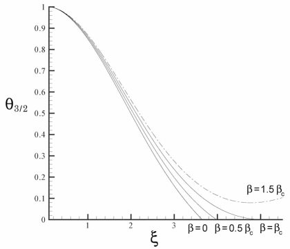
Figure 5: Same as in Fig.1, for $n=3/2$. The solutions asymptotically approach, at large $\xi$, the horizontal line $\theta_{3/2}=\beta^{2/3}$.

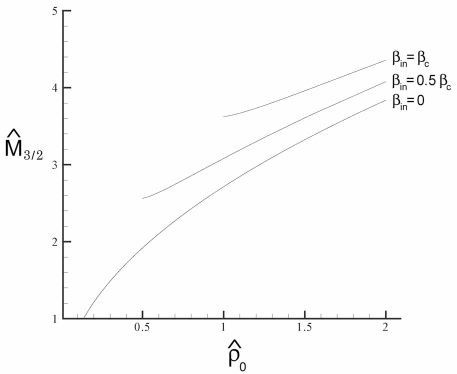
Figure 6: Same as in Fig.2, for $n=3/2$.

The density distribution for equilibrium configurations with $\beta=0,\,\,\beta=0.5\beta_{c},\,\,\beta=\beta_{c}$ is shown in Fig.5. The nonphysical solution at $\beta=1.5\beta_{c}$, which has not an outer boundary, is given by the dash-dot line. At large $\xi$, these solutions asymptotically approach the horizontal line $\theta_{3/2}=\beta^{2/3}$. The numerical solution of equation (49) gives $\beta_{c}=0.082$, $\xi_{out}=3.654,\,\,3.984,\,\,5.086$, for $\beta=0,\,\,\beta=0.5\beta_{c}=0.041,\,\,\beta=\beta_{c}=0.082$, respectively. In Fig.6 we show the behavior of $\hat{M}_{3/2}(\hat{\rho}_{0})|_{\Lambda}$, for different values of $\beta_{in}=0,\,\,\beta_{in}=0.5\beta_{c},\,\,\beta_{in}=\beta_{c}$, for which $\hat{M}_{3/2}=2.714,\,\,3.081,\,\,3.622$, at $\hat{\rho}_{0}=1$, respectively.

5 Application to the Local galaxy cluster

The question about the importance of DE on the dynamics of the Local Cluster (LC) was considered by Chernin (2001, 2008) and Chernin et al. (2009). Simple estimations confirm this importance and, for the presently accepted values of the DE density $\rho_{v}=(0.72\pm 0.03)\cdot 10^{-29}$ g/cm³, the mass of the local group, including the dark mater input, is between $M_{LC}\sim 3.5\cdot 10^{12}\,M_{\odot}$, according to Chernin et al. (2009), and $M_{LC}\sim 1.3\cdot 10^{12}\,M_{\odot}$, according to Karachentsev et al. (2006). The radius $R_{LC}$ of the LC is known even worse. It may be estimated by measuring the velocity dispersion $v_{t}$ of galaxies in LC and by the application of the virial theorem, so that $R_{LC}\sim\sqrt{(GM_{LC}/v_{t}})$. The velocity dispersion of the galaxies in LC, estimated by Karachentsev et al. (2006), resulted equal to $v_{t}=63$ km/s, very close to the value of the local Hubble constant $H=68$ km/s/Mpc (Karachentsev et al., 2006).

Similarity of this values indicates the great difficulties in dividing the measured velocities between regular and chaotic components. In addition, the indefiniteness increases because of the unknown level of the anisotropy in the velocity distribution. So, the radius of the LC may be estimated as $R_{LC}=(GM_{LC}/v_{t}^{2})=(1.5\div 4)$ Mpc, with a very high error box, which we cannot estimate properly. Chernin et al. (2009) give different intervals for the mass and radius of LC, without using the fixed value of $v_{t}$, but considering the whole picture of the distribution of the galaxy velocities. They obtained

$$1.2<M_{LC}<3.7\cdot 10^{12}\,{\rm M_{\odot}}\quad{\rm and}\quad 1.1<R_{v}<1.6\,{\rm Mpc}.$$ (51)

It is important to note that Chernin et al. (2009) identified the radius $R_{LC}$ of the LC with the radius $R_{v}$ of the zero-gravity force, which is identical with the one corresponding to our critical model with $\beta=\beta_{c}$, in which the average matter density is equal to $2\rho_{v}$, as we can see from (31). These estimations, while having very big observational errors, indicate the importance of the presently accepted value of DE density on the structure and dynamics of the outer parts of LC, and its vicinity.

Polytropic solutions with DE are not well appropriate for describing the LC, being the most mass concentrated in two giant objects: our Galaxy and M31 (Andromeda). The polytropic model may have better application to the rich galactic clusters, where the mass is more uniformly distributed among a large number of galaxies and the distribution of matter could be approximated by an averaged polytropic distribution. In this aspect, it is necessary to make more extended measurements of the galaxy velocities in the clusters and of their distribution over the cluster extension.

6 Conclusions

The density of DE, measured from SN Ia distributions and spectra of CMB fluctuations, imply the necessity to take into account such a contribution in calculations of the structure of galaxy clusters. We developed these calculations by considering simple polytropic models, in which it is possible to see how the model changes with increasing of the influence of DE.

Three different values of $n$ have been taken into account. Due to the presence of DE, only for central densities larger than a critical value $\rho_{c}$, depending of $n$, static solutions are found. We have derived the virial theorem for equilibrium configurations in presence of DE, finding expressions between different sorts of the energy in polytropic models.

We have analyzed the stability of equilibrium configurations in presence of DE using energetic method. It is shown, that DE increases the instability of the equilibrium configurations, working in the same direction as the influence of the general relativistic corrections. The presence of DE decrease the the level of relativity of a warm dark matter (WDM), at which it is still possible to form gravitationally bound configurations from WDM.

Finally, the observational indefiniteness in the parameters of LC does not permit to draw definite conclusions about the level of DE influence but, without any doubt, it indicates the dynamic importance of DE in the scale of the galaxy clusters.

References

- [1] Antonov, V.A. 1962, Vest. Leningr. Gos. Univ., 7, 135
- [2] Balaguera-Antolínez, A., Mota, D.F., Nowakowski, M. 2006, Class.Quant.Grav., 23, 4497
- [3] Balaguera-Antolínez, A., Mota, D.F., Nowakowski, M. 2007, MNRAS, 382, 621
- [4] Bisnovatyi-Kogan, G.S. 1998, ApJ, 497, 559
- [5] Bisnovatyi-Kogan, G.S. 2001, Stellar Physics. II. Stellar Structure and Stability (Heidelberg: Springer)
- [6] Chandrasekhar, S. 1939, An Introduction to the Study of Stellar Structure (Chicago: Univ. Chicago Press)
- [7] Chandrasekhar, S. 1964, ApJ, 140, 417
- [8] Chernin, A.D. 2001, Physics-Uspekhi, 44, 1099
- [9] Chernin, A.D. 2008, Physics-Uspekhi, 51, 267
- [10] Chernin, A.D. et al. 2009, astro-ph, 0902.3871v1
- [11] Eke, V.R, Cole, Sh.& Frenk, C.S. 1996, MNRAS, 282, 263
- [12] Karachentsev, I.D. et al. 2006, AJ, 131, 1361
- [13] Kofman, L.A. & Starobinsky, A.A. 1985, Sov. Astron. Lett., 11, 271
- [14] Landau, L.D. & Lifshitz, E.M. 1980, Statistical Physics, (Elmsford NY: Pergamon Press)
- [15] Lynden-Bell, D. & Wood, R. 1968, MNRAS, 138, 495
- [16] Lukash, V.N. & Rubakov, V.A. 2008, Physics-Uspekhi, 51, 283
- [17] McLaughlin, G. & Fuller, G. 1996, ApJ, 456, 71
- [18] Merafina, M. & Ruffini, R. 1989, Astron Ap., 221, 4
- [19] Perlmutter, S. et al. 1999, ApJ, 517, 565
- [20] Riess, A.G. et al. 1998, AJ, 116, 1009
- [21] Spergel, D.N. et al. 2003, APJ Suppl., 148, 175
- [22] Tegmark, M. et al. 2004, Phys. Rev. D, 69, 103501
- [23] de Vega, H.J. & Siebert, J.A. 2005, Nuclear Physics B, 707, 529
- [24] Zel’dovich, Ya.B. 1963, Voprosy Kosmogonii, 9, 157
- [25] Zel’dovich, Ya.B. & Novikov, I.D. 1966, Physics-Uspekhi, 8, 522