Incentive Compatible Influence Maximization in Social Networks and Application to Viral Marketing

Abstract

Information diffusion and influence maximization are important and extensively studied problems in social networks. Various models and algorithms have been proposed in the literature in the context of the influence maximization problem. A crucial assumption in all these studies is that the influence probabilities are known to the social planner. This assumption is unrealistic since the influence probabilities are usually private information of the individual agents and strategic agents may not reveal them truthfully. Moreover, the influence probabilities could vary significantly with the type of the information flowing in the network and the time at which the information is propagating in the network. In this paper, we use a mechanism design approach to elicit influence probabilities truthfully from the agents. We first work with a simple model, the influencer model, where we assume that each user knows the level of influence she has on her neighbors but this is private information. In the second model, the influencer-influencee model, which is more realistic, we determine influence probabilities by combining the probability values reported by the influencers and influencees. In the context of the first model, we present how VCG (Vickrey-Clarke-Groves) mechanisms could be used for truthfully eliciting the influence probabilities. Our main contribution is to design a scoring rule based mechanism in the context of the influencer-influencee model. In particular, we show the incentive compatibility of the mechanisms when the scoring rules are proper and propose a reverse weighted scoring rule based mechanism as an appropriate mechanism to use. We also discuss briefly the implementation of such a mechanism in viral marketing applications.

1 Introduction

Social networks are widespread and indeed provide an effective medium to propagate information and to market and advertise products. Examples of online social networks include facebook, twitter, linked in, orkut, etc. A social network, in a natural way, could be represented in the form of a graph in which an individual is represented as a node and there is an edge between two individuals if they are associated with each other.

Consider a situation in which a company has designed a new gaming console which it wants to market on a social network. As a marketing strategy, the company can select a small set of influential users to whom it provides the product for free. If these users like the product, then they will recommend it to their friends. These friends could get influenced by the users and will perhaps buy the product. Some of these friends will in turn recommend the product to their friends, leading to a marketing cascade. An online social network is an effective medium for launching such a marketing campaign because it has much information about the users as well as the relationship graph of users. The choice of an initial set of users is critical here because these initially selected users will decide the expected number of users that would get influenced ultimately. An important problem in this context is the influence maximization problem - given a social network graph and influence probabilities on each edge, how do we select a small set of initial users so as to maximize the number of users who get influenced. This problem has been solved in the literature as an optimization problem by assuming a suitable model of information diffusion. Various algorithms have been proposed to find the set of influential nodes in a social network efficiently [8, 3].

The current models for information diffusion process assume that the social planner knows the influence probabilities accurately. There are many reasons why this assumption is not true in practice. Consider an example, say a seller wants to sell a newly released book by some author and another seller wants to sell a tennis racket. Both the sellers decide to use viral marketing on a popular online social network to market these products. To do this the seller will have to find the values of influence probabilities on each edge and find the influential set of nodes to initiate the cascade process. Consider a typical user $u$ and her set of neighbors on the social network. See Figure 1. The influence probability of $u$ on each neighbor for a product say book need not be the same for another product say tennis racket. This is perhaps because $u$ is a novice tennis player but is good at English literature and her friends know this, however, this particular information is not available on this social networking site. Hence her friends will be influenced more by her recommendation of a novel to them than a tennis racket.

Figure 1: Variation of influence probabilities with product

Thus, the influence probabilities can vary drastically with the product being marketed, the time at which the recommendation is made, and perhaps many other factors. Building robust and accurate models for estimating the influence probabilities from the currently available data in online social networks is a difficult task. The best way to know the influence probabilities accurately is to elicit them truthfully from the users themselves. However, the users need not reveal the influence probabilities truthfully due to strategic reasons. For example, a user might misreport by projecting a higher level of influence on her friends in order to become a part of the initially active set.

The success of a viral marketing strategy or in general influence maximization is critically dependent on the initially chosen target set. This in turn depends on the accuracy of the influence probabilities. More generally, predicting information diffusion in a social network critically depends on knowing the influence probabilities.

In this paper we address the influence maximization problem in an incomplete information setting in which, influence probabilities are the private information. Our objective in this paper is to extract influence probabilities accurately using a mechanism design approach.

1.1 Relevant Work

Kempe, Kleinberg, and Tardos in [8] considered the algorithmic problem of influence maximization proposed by Domingos and Richardson in [6]. In this paper they proved that this problem is NP-hard even for simple models of information diffusion and for some of the more complex models, it is not even constant factor approximable. They gave a constant factor approximation algorithm for the independent cascade model by proving the sub-modularity of the influence function. The greedy algorithm they propose assumes that the influence probabilities are available to the algorithm. There are a number of algorithms proposed in the context of influence maximization in the recent years; we mention only two papers here: (a) Leskovec, Krause, and Guestrin [9] (b) Chen, Wang, and Yang [3]. These two papers also contain a rich set of related references.

Alon, Fischer, Procaccia, and Tennenholtz in [1] proposed a game theoretic model for truthfully choosing the agents that maximize the sum of indegrees in a directed graph. In the model they propose, they consider the outdegree of an agent as private information. The objective of each agent is to be among the set of nodes chosen by the algorithm. They propose several deterministic and randomized strategy-proof algorithms to achieve the objective of maximizing the sum of indegrees. The problem that we address in the present paper is different and more general. The objective of each agent in [1] is to maximize the number of neighbors that she is able to activate in the 0-1 cascade process. In our problem, on the other hand, the objective is to choose a set of agents that have maximum reachability.

A mechanism design based framework to extract the information from the agents has been proposed for ranking systems [2]. The authors study incentives in ranking systems, where agents try to maximize their position in the ranking, rather than to obtain a correct outcome. They consider several basic properties of ranking systems and characterize the conditions under which incentive compatible ranking systems exist. They show that in general no such system satisfying all the properties exists.

Dixit and Narahari in [5] proposed query incentive networks in which the nodes, along with the answer are aware of the quality of the answer. They proposed a game theoretic model of query incentive networks in which the quality of answer is the private information. They designed a scoring rule based mechanism to truthfully extract the quality of the answers from the agents along with the actual answer. In our work, we design the influencer-influencee model which is similar to the game theoretic model presented in [5] for query incentive networks. In [5] the rewards to the agents depend on the truthfulness of the quality of answers they report. In our problem, the payments to the agents depend on the truthfulness of the influence probabilities they report.

In the work by Goyal, Bonchi, and Lakshmanan in [7], the approach is to use a machine learning based approach for predicting the influence probabilities in social networks. Intuitively, the approach they consider is that if an individual $x$ takes a total of $a$ actions out of $b\leq a$ actions were performed by its neighbor $y$ before $x$, then there is a probability of $\frac{b}{a}$ that person $x$ will be influenced by $y$ in future. Here the “action” is the act of joining a community or group in a social network which does not involve any effort or monetary transfer. They validate the models they build on a real world data set.

To the best our knowledge, the model presented in this paper is the first one that captures strategic behavior of agents in the information diffusion process. Using this model, our aim is to elicit the true influence probabilities from the agents in order to accurately compute the set of highly influential nodes or predict the progress of information cascades.

1.2 Contributions and Outline

In this paper, we design mechanisms to extract influence probabilities truthfully from the users of a social network. We first work with a simple model, the influencer model, where we assume that each user knows the level of influence she has on her neighbors but this is private information. In the second model, the influencer-influencee model, which is more realistic, we determine influence probabilities by combining the probability values reported by the influencers and influencees.

The Influencer Model

First, we develop a game theoretic model for information diffusion process in which we ask only the influencer to reveal the influence probabilities on all outgoing edges. We propose a VCG (Vickrey-Clarke-Groves) mechanism [10] based approach. We show that, without using money or any payment scheme the ideal influence maximizing algorithm may not be incentive compatible. Then we show how a VCG mechanism based approach could be used.

The Influencer - Influencee Model

In this more general model, given an edge in the social network, we ask the influencer as well as the influencee to reveal the influence probability on the edge. This model is more realistic since, both the persons involved in a connection, will have information about the influence probability. We design a payment scheme in which we use scoring rules [11] to design the payment scheme. We show that it is a Nash equilibrium to report true influence probability in this mechanism. We also design the reverse weighted scoring rule (derived from the weighted scoring rule) which has several desirable properties which, standard scoring rules like the quadratic and spherical scoring rules do not possess.

Outline of the Paper

The rest of the paper is organized as follows. In the next section (Section 2), we provide essential preliminaries. We discuss the influencer model in Section 3 and the influencer-influencee model in Section 4. In Section 5, we briefly discuss how the influencer-influencee model could be implemented in a typical viral marketing scenario.

2 Preliminaries

Several probabilistic models have been proposed to model the spread of information in social networks. We give here a brief overview of the Independent Cascade Model. We will represent any social network by directed graph $G$. We will say that an individual (a node in the graph) is active if she is the adopter of the innovation or the behavior and inactive otherwise. We will assume that once an individual becomes active, she cannot switch back to being inactive.

2.1 Independent Cascade Model

Let $V=\{1,2,\ldots,n\}$ be the set of nodes in the social network. In this model we activate some subset of nodes $A$ initially. The information diffusion process unfolds in discrete time steps ($x=1,2,\ldots,$) as follows. Each node that becomes active at time step $x$ will try to activate each of its neighbors. A node will get the chance to activate its neighbors only once, that is at the time instant in which it becomes active. A node $i$ will successfully activate its neighbor $j$ with probability $p_{ij}$. Thus $p_{ij}$ is the probability that node $i$ will activate node $j$ conditioned on the event that node $j$ is inactive when node $i$ got activated. The successfully activated nodes at time instant $x$ can now activate their inactive neighbors at time instant $x+1$. This process ends when no more nodes get activated. Clearly this process will end in at most $n-1$ time steps, where $n$ is the number of nodes.

2.2 Influence Maximization Problem

First we define the notion of an influence function. Given an initially active set $A$ that is a subset of $V$ and influence probabilities, the influence function denoted by $\sigma(A)$ is the expected number of active nodes at the end of the diffusion process. The influence maximization problem is, given a parameter $k$, a social network graph $G$, and a model of information diffusion, to find a set of $k$ nodes in $G$ to be activated initially (also known as target set) such that, it will maximize the influence function $\sigma(A)$.

2.3 Scoring Rules

A scoring rule [11] is a sequence of scoring functions, $S_{1},S_{2},\ldots,S_{t}$, such that $S_{i}$ assigns a score $S_{i}(z)$ to every $z\in\Delta(T)$ where $\Delta(T)$ denotes the set of probability distributions on the set $T=\{1,2,\ldots,t\}$. Note that $z=(z_{1},z_{2},\ldots,z_{t})$ with $z_{i}\geq 0$ for $i=1,2,\ldots,t$ and $\sum_{i=1}^{t}z_{i}=1$. We will consider only real valued scoring rules. Scoring rules are primarily used for comparing the predicted distribution with the true observed one. Suppose $w\in\Delta(T)$ is the true observed distribution. Then the expected score of any general distribution $z\in\Delta(T)$ against $w$ is defined as

$$V(z|w)=\sum_{i=1}^{t}w_{i}S_{i}(z)$$

. The expected score loss is defined as

$$L(z|w)=V(w|w)-V(z|w)$$

A scoring rule $S_{1},S_{2},\ldots,S_{t}$ is called proper or incentive compatible if $\forall z,w\in\Delta(T)$ with $z\neq w$, $L(z|w)>0$. If the scoring rule is proper, then it is a best response for each agent to report its true probability distribution. The following are popular proper scoring rules discussed in the literature [11]:

• Quadratic scoring rule:

  $$S_{i}(z_{1},\ldots,z_{i},\ldots,z_{t})=2z_{i}-\sum_{j=1}^{t}z_{j}^{2}$$

• Logarithmic scoring rule:

  $$S_{i}(z_{1},\ldots,z_{i},\ldots,z_{t})=ln\leavevmode\nobreak\ \leavevmode\nobreak\ z_{i}$$

• Spherical scoring rule:

  $$S_{i}(z_{1},\ldots,z_{i},\ldots,z_{t})=\frac{z_{i}}{\sqrt{\sum_{j=1}^{t}z_{j}^{2}}}$$

• Weighted scoring rule

  $$S_{i}(z)=\frac{2i\cdot z_{i}-\sum_{j=1}^{t}z_{j}^{2}\cdot j}{t}$$

3 The Influencer Model

In this model we assume that only the influencer knows the influence probabilities and only the influencer is asked to report the probability values. The model is as follows.

• The social planner has the entire graph structure $(V,E)$ of the social network. The players in the game $V=\{1,\ldots,n\}$ are the users of the social network.

• Here each agent $i$ has the influence probability vector $\theta_{i}\in[0,1]^{\left|E\right|}$as her private information. The $jth$ component of $\theta_{i}$ will give the influence probability of $i$ on node $j$. Let $out(i)=\{j\in V|(i,j)\in E\}$ denote the set of successors of node $i$. The social planner does not know anything about the influence probability of node $i$ on its successors. For all other nodes, (non-neighbors of node $i$), the influence probability will be zero and this is known to the social planner as the social planner has the structure of the graph. Prior to starting the information diffusion process, the social planner asks each agent to report her influence probabilities. The reports from the agents may or may not be truthful.

• Given the reported influence probabilities, the social planner now computes the target set using an influence maximization algorithm. Let this target set be $A$.

• Let $\theta\in[0,1]^{\left|E\right|}$ be the true influence probability vector, representing the influence probability on each edge of the graph. Then the utility of a player when the social planner chooses a target set $A$ is the expected number of neighbors activated by that player. Also, without involving payments, the valuation function for each agent is equal to its utility that is,

  $$u_{i}(\theta,A)=v_{i}(\theta,A)$$

  Thus utility is proportional to the expected number of neighbors an agent is able to activate, given the target set.

Here the valuation function represents the preferences of the agents over the target set chosen by the social planner.

3.1 A VCG Mechanism Based Approach

Consider the exact influence maximization problem which optimizes the influence function. It has been proven in [8] that this problem is NP-hard. Even if we are given that the algorithm to choose the target set finds the optimal solution, we can come up with an example in which the agents would prefer to lie about their preferences and still be better off. One such example is given in the next subsection. We can make this algorithm incentive compatible by introducing appropriate incentives to the agents. An immediate and natural approach is to use the VCG (Vickrey-Clarke-Groves) mechanisms [10]. We shall, in particular, explore the use of the Clarke payment rule [4] to make this mechanism incentive compatible. The utility of the agents with Clarke payments will take the form:

$$u_{i}(\theta,A)=v_{i}(A)+p_{i}(v_{1},v_{2},...,v_{n})$$

where $p_{i}$ is the discount offered to agent $i$ by the social planner.

In order to design a VCG mechanism, we first need to prove that the social choice function is allocatively efficient. Note that, in our framework, the social choice function is precisely the algorithm being used to choose the target set. We will first prove the following useful lemma which will immediately imply that the exact influence maximization algorithm is allocatively efficient. To prove the lemma, we will first describe an equivalent view of the independent cascade model given by Kempe, Kleinberg, and Tardos in [8].

The influence probability of node $i$ on $j$ denoted by $\theta_{ij}$ gives the probability that node $i$ will activate $j$ given that node $j$ will be inactive at the instant when node $i$ becomes active. This event can be viewed as the flip of a biased coin. In the process, let us say we flip the coins on all the edges before the start of the cascade process and check the result of the coin flip only when a node becomes active and its neighboring node is inactive. This change will not affect the final result and it is equivalent to the original cascade process. We call the edges on which the coin flip resulted in heads as live edges and the remaining edges as blocked. Given this equivalent view, if we fix the outcomes of all coin flips and initially active set of nodes $A$, then we will get a graph in which some edges are live and the rest are blocked, depending on the outcome. Clearly in this graph, if we run the cascade process, then the number of nodes that are active will be the number of nodes that are reachable from set $A$ on a path that consists of only live edges.

Thus we will consider a sample space $S$ in which each sample point corresponds to one possible outcome of all the coin flips. If $X$ denotes one such fixed outcome of coin flips, we define $\sigma_{X}(A)$ to be the number of active nodes at the end of the cascade process for the fixed outcome $X$ and target set $A$. Then $\sigma(A)$, the expected number of active nodes at the end of the cascade process, is given by:

$$\sigma(A)=\sum_{X\in S}P[X]\sigma_{X}(A)$$

Given this formula for $\sigma(A)$, we can now prove the following lemma.

lemma 1.

Given a target set $A$, then

$$\sigma(A)=\sum_{i=1}^{n}v_{i}(\theta,A)+\left|A\right|$$

where $v_{i}$ is the valuation function of agent $i$ which is equal to the expected number of neighbors activated by that agent.

Proof.

Fix a sample point $X$ from the sample space $S$ of all possible coin flips on the edges. Consider an arbitrary node $i$ in the graph. Let $v_{i_{X}}(A)$ be the number of neighbors activated by node $i$ for outcome $X$. More concretely, let us define $d(A,v)$ where $A\subseteq V$ and $v\in V$ as the shortest path distance between $A$ and a node $v$. Thus, $d(A,v)=0$ if $v\in A$. Let, $R_{Av}=\{u\in V|(u,v)\in E_{X}\wedge d(A,u)+1=d(A,v)\}$ where, $E_{X}$ is the edge set that is active for the outcome $X$. $R_{Av}$ is the set of nodes that are lying on the shortest path from set $A$ to node $v$. Thus, we define

$$v_{i_{X}}(A)=\left|\{v\in N(i)|i\in R_{Av}\wedge i\succeq j\,\forall j\in R_{Av}\}\right|$$

where, the ordering $\succeq$ is lexicographic (we are breaking the ties in favor of the node with the highest lexicographic order). Also lexicographic ordering ensures that a node is activated deterministically by exactly one node for a fixed outcome $X$. Then we have,

$$\sigma_{X}(A)=\sum_{i=1}^{n}v_{i_{X}}(A)+\left|A\right|$$

Also we can see that

$$\sum_{i=1}^{n}v_{i}(\theta,A)+\left|A\right|=\sum_{X\in S}P[X]\{\sum_{i=1}^{n}v_{i_{X}}(A)+\left|A\right|\}$$

Since $\sum_{X\in S}P[X]=1$, we have

$$\sum_{i=1}^{n}v_{i}(\theta,A)+\left|A\right|=\sum_{X\in S}P[X]\sigma_{X}(A)$$

This implies

$$\sum_{i=1}^{n}v_{i}(\theta,A)+\left|A\right|=\sigma(A)$$

∎

Thus, by using Lemma 1, we can say that an influence maximization algorithm that finds the exact optimal solution is allocatively efficient and hence VCG payments will give us strategy proof mechanism for this algorithm [10]. Thus with VCG payments, the utility for each agent will be :

$$u_{i}(\theta,A)=v_{i}(A)+\sum_{j\neq i}v_{j}(A)-h(v_{1},...v_{i-1},v_{i+1},...v_{n})$$

Here $h$ is some function independent of $v_{i}$. Thus we have the following result:

Theorem 1.

The influence maximization algorithm that finds an exact optimal solution is allocatively efficient and hence is dominant strategy incentive compatible under VCG payments.

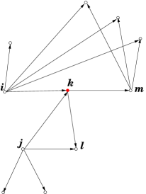
Figure 2: A stylized social network

3.2 An Illustrative Example

We now provide a simple example to illustrate how the proposed model functions. Consider a simple social network graph as shown in Figure 2. Assume that the true influence probabilities are all $1$ in the graph and the algorithm for target set selection is an exact influence maximizing algorithm. Note that all the agents in the network have complete information about the network. If we want to choose only one node as the target set, then clearly node $j$ will be chosen, because $\sigma(\{j\})=8$, which represents the maximum influence among all nodes present, as can be seen from the figure. Now assume that, all nodes except node $k$ report their true influence probabilities. Consider node $k$, if this node reports its true influence, then node $j$ will be chosen as target set and its utility will be $1$, because she will only be able to influence node $m$. This is because when the cascade reaches node $k$ at time $x=1$, then till that time its neighbor node $l$ would have already been influenced by node $j$ at time $t=0$. Now if node $k$ lies about its influence on node $m$ as $0$, then node $i$ will be chosen as the influence maximizing target set. For this target set, the utility of agent $k$ will be $2$ but now the influence function will be $\sigma(\{i\})=7$. Thus agent $k$ is better off by lying rather than reporting the truth. Hence the exact influence maximization algorithm is not incentive compatible without payments.

Now assume that we include the Clarke payment scheme in this scenario and $h(v_{1},\ldots,v_{i-1},v_{i+1},\ldots,v_{n})=0$. If node $j$ is chosen as the target set then agent $k$ will be able to influence agent $m$ and she will get a monetary payment of $7$ units, thus total utility will be $8$ and if any other node is chosen as the target set, then node $k^{\prime}s$ payoff will be lower.

Note: It may be noted that the greedy algorithm proposed by Kempe, Kleinberg, and Tardos in [8] is the same as the exact influence maximization algorithm in the special case $|A|=1$. Thus the above example also shows that the greedy algorithm is not incentive compatible. We can construct examples for other heuristic based algorithms like the high degree heuristics [8], degree discount heuristics [3] etc., to illustrate that they are not incentive compatible. All these algorithms use the information reported by the agents directly to select the target set. Thus, none of these algorithms are strategy-proof. However the randomized algorithm in which we select the nodes in the target set uniformly randomly is strategy-proof. But the expected influence of this algorithm is low as shown by the experiments done in [8].

4 Influencer - Influencee Model

The obvious limitation of the influencer model discussed above is the restricted assumption that the influencer alone decides the influence probabilities. In a real world social network, given a social connection between two individuals, both the individuals will have information about different aspects and properties of the connection. The influencer-influencee model tries to leverage this fact in designing an incentive compatible mechanism for eliciting influence probabilities. An advantage of the mechanisms designed with this model is that the agents need not know any information beyond its neighborhood. We now describe this model and propose a mechanism based on scoring rules for truthfully eliciting influence probabilities.

4.1 The Model

• Given a directed edge $(i,j)$ in the social network, the social planner will ask:

  • agent $i$ (the influencer) to report her influence probability $\theta_{ij}$ on $j$ and

  • agent $j$ (the influencee) to report agent $i^{\prime}s$ influence on her.

  Thus the social planner will ask each agent to reveal the probability distribution over each edge which is incident on it and which is emanating from it. We can consider the activation probability on each edge as a probability distribution over the set $\{active,inactive\}$.

• Given these influence probabilities, the social planner will compute:

  • the influence maximizing target set using an influence maximization algorithm and

  • the amount of discount to be given to the agents based on their reported probability distribution on edges using a scoring rule based approach that will be described soon.

• Consider an agent $i$. Let $out(i)=\{j|(i,j)\in E\}$ and $in(i)=\{j|(j,i)\in E\}$. Thus agent $i$ acts as influencer to nodes in the set $out(i)$ and acts as the influencee for the nodes in set
  $in(i)$. In this model an assumption is that agent $i$ knows the influence probabilities on the edges that are incident on $i$ and that are emanating from $i$. Thus agent only knows about the influence probabilities in its neighborhood and nothing beyond that.

• Also no agent knows what influence probability is reported by the agents in its neighborhood. The only way an agent can predict the reported probability by its neighbor is by her own assessment of it. Thus we assume that for any given pair of nodes $i$ and $j$ having edge $(i,j)$ between them, the conditional probability distribution function $P(\theta_{ij}^{j}|\theta_{ij}^{i})$ which has all the probability mass concentrated at $\theta_{ij}^{j}=\theta_{ij}^{i}$.

• Here we discretize the continuous interval [0,1] into $\frac{1}{1+\epsilon}$ equally spaced numbers and agents will have to report the influence probability by quoting one of the $\frac{1}{1+\epsilon}$ numbers. More concretely, given set $T=\{1,2,\ldots,t\}$ we define $z\in\{0,\epsilon,2\epsilon,...,1\}^{t}$ such that $\sum_{i=1}^{t}z_{i}=1$. For the case of our problem, $T=\{active,inactive\}$, thus agents will only have to report one number $\theta_{ij}\in\{0,\epsilon,2\epsilon,...,1\}$.

Based on this model we will now design a scoring rule based payment schemes.

4.2 A Scoring Rule Based Mechanism

We now consider a scoring rule based payment scheme in which we incentivize agents for reporting the true probability distribution on each edge. In this mechanism, the payment to an agent $i$ depends on the truthfulness of the distribution she reveals on edges incident on $i$ as well as on the edges emanating from $i$.

First we state a lemma without proof. The lemma quantifies the amount of loss that an agent suffers by not reporting its true type.

lemma 2.

If $w,z\in\{0,\epsilon,2\epsilon,...,1\}^{t}$, $0<\epsilon\leq 1$ such that $\sum_{i=1}^{t}w_{i}=1$ and $\sum_{i=1}^{t}z_{i}=1$ and $z_{i}=w_{i}\pm\epsilon$ for at least one integer $1\leq i\leq t$, then

• For quadratic scoring rule

  $$V(z|w)\leq V(w|w)-2\epsilon{}^{2}$$

• For the spherical scoring rule

  $$V(z|w)\leq V(w|w)-1.5\epsilon{}^{2}$$

• For weighted scoring rule

  $$V(z|w)\leq V(w|w)-\epsilon{}^{2}$$

We develop the mechanism assuming the quadratic scoring rule. A similar development will follow for other proper scoring rules. In the proposed mechanism, the payment received by an agent $i$ is given by

$$\left(v_{i}(A,\theta)+\frac{d_{i}^{2}}{2\epsilon^{2}}\right)\Biggl{(}\sum_{j\in in(i)}V_{ji}^{i}(\hat{\theta_{ji}^{j}}|\hat{\theta_{ji}^{i}})+\sum_{j\in out(i)}V_{ij}^{i}(\hat{\theta_{ij}^{j}}|\hat{\theta_{ij}^{i}})\Biggr{)}$$

where $d_{i}$ is the degree of agent $i$, $V_{ij}^{i}()$ is the expected score that agent $i$ gets for reporting the distribution $\hat{\theta_{ij}^{i}}$ on the edge $(i,j)$. We are now in a position to state and prove the main result of this paper. The theorem specifically mentions quadratic scoring rule for the sake of convenience but will hold for any proper scoring rule.

Theorem 2.

Given the influencer-influencee model, reporting true probability distributions is a Nash equilibrium in a scoring rule based mechanism with quadratic scoring rule.

Proof.

We will first consider the strategic behavior of any arbitrary agent $i$ considering only the agents in the set $S=in(i)\cup out(i)$. In the payment scheme, the agents belonging to the set $V\setminus S$ can only affect the valuation $v_{i}(A,\theta)$. The expected payoff an agent $i$ gets is given by

$$\sum_{j\in in(i)}\sum_{\theta_{ji}=0}^{1}P(\theta_{ji}^{j}|\theta_{ji}^{i})v_{i}(A,\theta)V_{ji}^{i}(\hat{\theta_{ji}^{j}}|\hat{\theta_{ji}^{i}})+$$

$$\sum_{j\in out(i)}\sum_{\theta_{ij}=0}^{1}P(\theta_{ij}^{j}|\theta_{ij}^{i})v_{i}(A,\theta)V_{ij}^{i}(\hat{\theta_{ij}^{j}}|\hat{\theta_{ij}^{i}})+$$

$$\frac{d_{i}^{2}}{2\epsilon^{2}}\Biggl{(}\sum_{j\in in(i)}\sum_{\theta_{ji}=0}^{1}P(\theta_{ji}^{j}|\theta_{ji}^{i})V_{ji}^{i}(\hat{\theta_{ji}^{j}}|\hat{\theta_{ji}^{i}})+$$

$$\sum_{j\in out(i)}\sum_{\theta_{ij}=0}^{1}P(\theta_{ij}^{j}|\theta_{ij}^{i})V_{ij}^{i}(\hat{\theta_{ij}^{j}}|\hat{\theta_{ij}^{i}})\Biggr{)}$$

Note that the valuation $v_{i}(A,\theta)$ is dependent on the assessment of the influence probabilities by agent $i$ in its neighborhood. Every agent will now try to maximize the expected payoff by considering the strategies of agents in its neighborhood. If all the agents in the neighborhood are truthful then we have

$$\sum_{j\in in(i)}\sum_{\theta_{ji}=0}^{1}P(\theta_{ji}|\theta_{ji}^{i})v_{i}(A,\theta)V_{ji}^{i}(\theta_{ji}|\hat{\theta_{ji}^{i}})+$$

$$\sum_{j\in out(i)}\sum_{\theta_{ij}=0}^{1}P(\theta_{ij}|\theta_{ij}^{i})v_{i}(A,\theta)V_{ij}^{i}(\theta_{ij}|\hat{\theta_{ij}^{i}})+$$

$$\frac{d_{i}^{2}}{2\epsilon^{2}}\Biggl{(}\sum_{j\in in(i)}\sum_{\theta_{ji}=0}^{1}P(\theta_{ji}|\theta_{ji}^{i})V_{ji}^{i}(\theta_{ji}|\hat{\theta_{ji}^{i}})+$$

$$\sum_{j\in out(i)}\sum_{\theta_{ij}=0}^{1}P(\theta_{ij}|\theta_{ij}^{i})V_{ij}^{i}(\theta_{ij}|\hat{\theta_{ij}^{i}})\Biggr{)}$$

Now consider the expression

$$\left(v_{i}(A,\theta)+\frac{d_{i}^{2}}{2\epsilon^{2}}\right)\Biggl{(}\sum_{j\in in(i)}V_{ji}^{i}(\theta_{ji}|\hat{\theta_{ji}^{i}})+\sum_{j\in out(i)}V_{ij}^{i}(\theta_{ij}|\hat{\theta_{ij}^{i}})\Biggr{)}$$

Now Let

$$\beta=\sum_{j\in in(i)}V_{ji}^{i}(\theta_{ji}|\theta_{ji})+\sum_{j\in out(i)}V_{ij}^{i}(\theta_{ij}|\theta_{ij})$$

Thus $\beta$ is the expected score agent $i$ gets when she reports the true distribution over all the edges. Also, by probability mass assumption, this is the expected score she will receive when she reports truthfully.

Thus, if an agent is truthful then, she will receive a payoff given by

$$\left(v_{i}(A,\theta)+\frac{d_{i}^{2}}{2\epsilon^{2}}\right)\beta$$

Let $v_{i}(A,\theta)$ be the true valuation of an agent and $v^{\prime}_{i}(A,\theta)$ the valuation when agent lies. That is when agent reports some $\hat{\theta_{ij}^{i}}\neq\theta_{ij}$. Consider the utility of an agent when she lies on only one of the edges

$$\left(v^{\prime}_{i}(A,\theta)+\frac{d_{i}^{2}}{2\epsilon^{2}}\right)\left(\beta-2\epsilon^{2}\right)$$

When an agent reports a probability value that is $\pm\epsilon$ away from the true probability value, the quadratic scoring rule (Lemma 2) ensures that the agent gets payoff lower by $2\epsilon^{2}$ for that edge. Now, we assume the worst case scenario in which agent gains maximum by reporting the false probability value on only a single edge and that too minimum possible deviation from the true value, Since we divide the [0,1] probability interval into $1/\epsilon$ numbers, agent $i$ has to report the probability value that is at least $\epsilon$ away from the true probability value. That is, agent $i$ will have to report some probability value $\hat{\theta_{ij}^{i}}=\theta_{ij}\pm\epsilon$. This gives us $\left(\beta-2\epsilon^{2}\right)$.

An agent cannot get a higher score for lying, as the quadratic scoring rule is incentive compatible. Thus the agent can gain only in the valuation part. Now by reporting a false probability distribution, the agent can get a valuation greater than true valuation by say $\delta$ that is,

$$v^{\prime}_{i}(A,\theta)=v_{i}(A,\theta)+\delta$$

where $\delta\in[0,\sum_{j\in out(i)}\theta_{ij}-v_{i}(A,\theta)]$. Thus by reporting a false probability value, an agent gets a payoff of

$$\left(v_{i}(A,\theta)+\delta+\frac{d_{i}^{2}}{2\epsilon^{2}}\right)\left(\beta-2\epsilon^{2}\right)$$

Thus for the agent to remain truthful we require that

$$\left(v_{i}(A,\theta)+\frac{d_{i}^{2}}{2\epsilon^{2}}\right)\beta\geq\left(v_{i}(A,\theta)+\delta+\frac{d_{i}^{2}}{2\epsilon^{2}}\right)\left(\beta-2\epsilon^{2}\right)$$

$$\Longrightarrow d_{i}^{2}+\left(v_{i}(A,\theta)+\delta\right)2\epsilon^{2}\geq\delta\beta$$

As the agents are rational $d_{i}\geq\delta\geq 0$. Also, for the quadratic scoring rule the maximum possible expected payoff for each edge will be at most 1. Thus, $\beta\leq d_{i}$. Now, we have $\delta\beta\leq d_{i}^{2}$ and $\left(v_{i}(A,\theta)+\delta\right)2\epsilon^{2}\geq 0$. Thus, it is a best response strategy for an agent to report truthfully when the agents in its neighborhood are truthful.

We still have to resolve the case for agents belonging to the set $V\setminus S$. Note that these agents only affect the valuation of agent $i$. In the above analysis, the best response strategy for an agent was derived by assuming that with minimum possible deviation from reporting true probability values, agent $i$ is able to gain maximum possible valuation. Thus even if agents in $V\setminus S$ report any arbitrary values, a best response strategy for agent $i$ is to report truthfully. Thus without knowing the strategy of agents in set $V\setminus S$, the best response for an agent $i$ is to report truthfully. Thus reporting true influence probabilities is a Nash equilibrium in this mechanism. ∎

Note that the social planner will have to choose the value of $\epsilon$ which will decide the accuracy of the probability values extracted from the users. Smaller the value of $\epsilon$, greater the payment the seller will have to make to the users. The main advantage of this mechanism is that the seller can use any of the algorithms to select the target set. The agents will be truthful regardless of which target set is chosen.

A similar payment scheme will work with other scoring rules namely logarithmic, spherical, and weighted scoring rule. We omit this due to constraints of space.

4.3 The Reverse Weighted Scoring Rule

Standard proper scoring rules such as quadratic, logarithmic, spherical, and weighted scoring rules have a serious limitation in the current context. If the influence probability on an edge is zero, all these scoring rules will give an expected score of 1. Thus, if the social network is the empty graph in which all the edges are inactive, these standard payment schemes will give maximum possible expected score. We now propose the following reverse weighted scoring rule to overcome the above limitation:

$$S_{i}(z)=2z_{i}(t-i)-\sum_{j=1}^{t}z_{j}^{2}(t-j)$$

We now show that this scoring rule is proper.

lemma 3.

The reverse weighted scoring rule is a proper scoring rule.

Proof.

Consider the expression for the expected score of reverse weighted scoring rule, given distributions z and w:

$$V(z|w)=\sum_{i=1}^{t}w_{i}S_{i}(z)$$

$$=\frac{2\sum_{i=1}^{t}w_{i}z_{i}(t-i)-\sum_{i=1}^{t}z_{i}^{2}(t-i)}{t}$$

$$V(w|w)=\sum_{i=1}^{t}w_{i}S_{i}(w)$$

$$=\frac{2\sum_{i=1}^{t}w_{i}^{2}(t-i)-\sum_{i=1}^{t}w_{i}^{2}(t-i)}{t}$$

$$=\frac{2\sum_{i=1}^{t}w_{i}^{2}(t-i)}{t}$$

$$L(z|w)=V(w|w)-V(z|w)$$

$$=\frac{\sum_{i=1}^{t}(w_{i}-z_{i})^{2}(t-i)}{t}$$

since, $i\leq t$ the loss is always positive. Thus, reverse weighted scoring rule is proper. ∎

It can also be shown that the the reverse weighted scoring rule also satisfies the following desirable properties:

1. The expected score is proportional to the influence probability.

2. If $\theta_{ij}=0$ then the expected score for the edge $(i,j)$ to both the agents $u$ and $v$ is zero. That is, $V_{ij}^{i}(\theta_{ij}^{j}|\theta_{ij}^{i})=V_{ij}^{j}(\theta_{ij}^{i}|\theta_{ij}^{j})=0$ if $\theta_{ij}=0$.

Property 1 is desirable because the social planner would want to reward the agent which revealed the social connection through which the product can be sold with high probability. Property 2 ensures that an agent does not get anything for revealing a social connection through which the product cannot be sold.

5 Implementation in Viral Marketing Scenarios

Since the mechanisms presented under the influencer-influencee model involve payments, the influence maximization process will involve monetary transfers. We now discuss the implementation of the mechanism in the context of viral marketing in an online social network like facebook, orkut, etc.

Consider that a seller wants to market a certain product through a given social network. The seller can now ask each user in the social network to reveal her influence on each of the users in their friends list. Users have incentive to participate in this mechanism because each user will get a certain positive payment based on the influence probabilities they report. The seller can ask each agent to report the influence probability by developing the application on the social network. There are a large number of applications on the social networks like orkut, facebook etc. which users use extensively for playing games and socializing online.

In an online social network like facebook, for example, if a user is interested in the product to be sold, then she can grant the access to the application. Now, this application will have full access to the friends list and other profile information of the user that is public. Thus such an application can be implemented in an online social network without any privacy issues. The seller will first have to fix the level of accuracy that she needs before starting the information extraction process.

Now, given the influence probabilities, the application will compute the influence maximizing target set. The application will also compute the payment to be made to the user. This payment can be made in the form of a discount (up to 100 percent) on the product or discount coupons or complimentary gifts or a combination of these. The marketing and sale of the product will now proceed as in the independent cascade process and users will get appropriate discounts based on the reported influence probabilities. Since the payment scheme ensures incentive compatibility, every user will truthfully reveal the information to the seller via the application.

6 Summary and Future Work

In this paper, we have proposed mechanisms for eliciting influence probabilities truthfully in a social network. Influence maximization in general and viral marketing in particular are the immediate applications. The work opens up several interesting questions:

• In this model we assumed that the influence probability is known exactly to the agents. We can relax this assumption and assume that agents know the belief probability rather than exact influence probability.

• In the influencer model, does there exist an incentive compatible algorithm having a constant factor approximation ratio with or without payments?

• In the influencer model, does there exist a heuristic based incentive compatible algorithm which may not have theoretical guarantees about the approximation but in a practical sense it performs well?

• In the influencer-influencee model, the payments depend on $\epsilon$ which decides the accuracy of the probability distribution. The higher the accuracy is required, the higher is the payment to be made to the user. An interesting direction of future research would be to design incentive compatible mechanisms that are independent of this factor.

References

- [1] N. Alon, F. Fischer, A. Procaccia, and M. Tennenholtz. Sum of us: Strategyproof selection from the selectors. Working Paper, 2010.
- [2] A. Altman and M. Tennenholtz. Incentive compatible ranking systems. Proceedings of the 6th International Conference on Autonomous agents and Multiagent Systems, AAMAS, article no. 5, 2007.
- [3] W. Chen, Y. Wang, and S. Yang. Efficient influence maximization in social networks. Proceedings of the 15th ACM SIGKDD Conference on Knowledge Discovery and Data mining, KDD, pages 199–208, 2003.
- [4] E. Clarke. Multi-part pricing of public goods. Public Choice, 11(1):17–23, 1971.
- [5] D. Dixit and Y. Narahari. Quality concious and truthful query incentive networks. 5th Workshop on Internet and Network Economics, WINE, pages 386–397, 2009.
- [6] P. Domingos and M. Richardson. Mining the network value of customers. Proceedings of the 7th ACM SIGKDD Conference on Knowledge Discovery and Data mining, KDD, pages 47–56, 2001.
- [7] A. Goyal, F. Bonchi, and L. Lakshmanan. Learning influence probabilities in social networks. Proceedings of The Third ACM International Conference on Web Search and Data Mining, WSDM, pages 241–250, 2010.
- [8] D. Kempe, J. Kleinberg, and E. Tardos. Maximizing spread of influence through a social network. Proceedings of the 9th ACM SIGKDD Conference on Knowledge Discovery and Data mining, KDD, pages 137–146, 2003.
- [9] J. Leskovec, L. Adamic, and B. Huberman. The dynamics of viral marketing. ACM Transactions on the Web, 1(1), 2007.
- [10] A. Mas-Colell, M. Whinston, and J. Green. Oxford University Press, New York, 1995.
- [11] R. Selten. Axiomatic characterization of the quadratic scoring rule. Discussion Paper Serie B 390, University of Bonn, Germany, 1996.