LO vs NLO comparisons for : MC as a tool for background determination for NP searches at LHC
Abstract
The leptonic decays of the heavy gauge bosons W and/or Z provide a clear experimental signature at hadron colliders. The production of accompanying jets is an excellent signal to probe QCD, while also being the main background to many searches for new physics. Describing the complex final state of W or Z + jets is a theoretical challenge with most existing calculations combining matrix elements for high energy jet production with a parton shower for lower energy jet production. We focus on two models: , which uses Leading Order matrix elements for boson and jet production; and with , which uses a Next-To-Leading Order Matrix element for Z production. In order to isolate the impact of the matrix elements for jet production, it is first essential to constrain the differences in the rest of the calculation in each case: specifically, the Multiple Parton Interaction models, and the tuning of the parton shower interfaced to the matrix elements. We test all three aspects of these models against data from the Tevatron, and perform a study of some basic kinematic variables at the LHC energy.
Flavia de Almeida Dias111flavia.dias@cern.ch
Instituto de Fisica Teorica, Universidade Estadual Paulista
Emily Nurse222nurse@hep.ucl.ac.uk
Dept. of Physics and Astronomy, University College London
Gavin Hesketh333gavin.hesketh@cern.ch
Dept. of Physics and Astronomy, University College London
1 Introduction
The leptonic decays of the heavy gauge bosons and/or accompanied by jets, and , offer search channels for new interactions of particles in high energy collisions. Many extensions of the Standard Model predict new particles with electroweak (EWK) couplings that decay into the SM gauge bosons , , and , accompanied by jets. Any production of new heavy particles with quantum numbers conserved by the strong interaction and EWK couplings is likely to contribute to signatures with one or more EWK gauge bosons; additional jets will always be present at some level from initial-state radiation, and may also be products of cascade decays of new heavy particles. and are backgrounds to most supersymmetry searches in final states with leptons, jets and missing transverse energy. The signal is an irreducible background to inclusive hadronic searches of Dark Matter, based on jets and missing energy (MET). W or Z + jets is also a major background for Higgs searches.
In the context of the SM, the study of the production of electroweak bosons with allows for tests of perturbative QCD. The production cross section scales approximately with the strong coupling constant for each additional jet. While current theoretical predictions at leading order (LO) and next to leading order (NLO) are in good agreement with data at the Tevatron, comparison at the higher energy of the LHC, and at higher jet multiplicities are needed. Inclusive and differential cross sections access the parameters of the perturbative expansion, such as the renormalization and the factorization scales, as well as the parton density functions (PDFs), through the and distributions of the vector bosons and the associated jets. Predicting all these quantities and comparing them to the Tevatron data has already produced several improvements in the calculation and generation techniques, such as the introduction of generators based on the LO calculations of matrix-element (ME) for the associated jet production, and the definition of several matching procedures to the parton-shower generators.
In this paper we make a comparative study of ME+PS Monte Carlo generators ( and ) with an NLO calculation (), validated with Tevatron D0 and CDF data, and generated at the LHC energy. This will serve as a preparatory MC study of the major SM backgrounds for the regions that are relevant to New Physics searches.
2 Matrix Elements Corrections / Parton Shower
The Parton Shower (PS) technique is a collinear approximation of the description of parton splittings in QCD radiation that accompanies hard scattering processes.
However, although it provides a good description of low observables, it usually fails to fill the phase space (can’t emit anything above the factorisation scale by construction) and in the hard region (close to the factorisation scale) this approximation is simply no good anymore. One way to improve the description of kinematical observables is to add a Matrix Element (ME) correction for the extra emissions. This can be implemented in different ways, as will be described in each generator section.
2.1
The generator uses the improved CKKW Matrix Element - Parton Shower merging [1] that relies on a separation of the event phase space in two separated regions, defined by a choice of scale. Above the chosen scale, all radiation must be produced by the Matrix Elements, and below the chosen scale all radiation produced by the Parton Shower. In matching these two regions to provide full phase space coverage, overlaps such as a parton shower emission in the scale range covered by the Matrix Element, must be removed [2].
The basic steps in the algorithm implementation are [2]:
-
•
Events are generated based on the matrix elements for W/Z + k jets, where k = 0, … N. The Matrix Element jets are required to be above the merging scale, .
-
•
The event is then reconstructed back from the final state particles. Particles are combined in the most likely combinations according to the parton shower probabilities.
-
•
Events are then passed to the parton shower, which is allowed to generate radiation from any part of the process.
-
•
The shower is then analyzed, and any events in which parton shower produces an emission above the scale are vetoed, leading to a rejection of the full event. This process is called Sudakov rejection.
The generator automatizes the generation of inclusive samples, combining ME for different parton multiplicities with PS and hadronization. Some parameters related to the ME and PS calculations have to be set accordingly.
2.2
The aim of the ME corrections in the PS on is to correct for two deficiencies in the shower algorithm: to populate the uncovered region of high in the phase space (non-soft non-collinear), and to correct the populated region, where the extrapolation away from the soft and collinear limits is not perfect. These corrections are called the hard and soft matrix element corrections respectively [3].
Soft Matrix Element Corrections
The soft correction is derived by comparing the probability density that the resolvable parton is emitted into a region of the phase space in the PS approximation (quasi-collinear limit), and the exact ME calculation. A simple veto algorithm is then be applied to the parton shower to reproduce the matrix element distribution, which relies on there always being more parton shower emissions than matrix element emissions. This is ensured simply by enhancing the emission probability of the parton shower with a constant factor [3].
The correction is applied to the hardest emission so far in the shower, to ensure that the leading order expansion of the shower distribution agrees with the leading order matrix element, and that the hardest (i.e. furthest from the soft and collinear limits) emission reproduces it [4].
Hard Matrix Element Corrections
The hard ME corrections aim to populate the high region that the PS leaves uncovered. This domain of the phase space should have radiation distributed according to the exact tree level ME for this extra emission, and as the Parton Shower does not populate this region, a different approach is needed to achieve this. Prior to any showering, the algorithm checks if the required ME is available for the hard process. Then, a point is generated in the appropriate region of phase space, with a probability based on a sampling of the integrand. The differential cross section associated with this point is then calculated and multiplied by a phase space volume factor, giving the event weight. The emission is accepted if the weight is less than a uniformly distributed random number in the [0,1] interval, and the momenta of the new parton configuration is processed by the shower as normal [3].
3 Next to Leading Order Methods
Both and described above include dominant QCD effects with leading order matrix elements combined with a leading logarithmic parton shower. However, higher order calculations are required to match the precision of current data measurements. Going even one step beyond the leading order is already a complex task: the initial hard process should be implemented in NLO; and shower development would have to be improved in next to leading logarithmic accuracy in collinear and soft structure. An intermediate step has already been developed: keeping the leading logarithmic order for the shower approximation, while improving the treatment of the hard emission to NLO accuracy (NLO+PS approach). We test one such generator: .
3.1
In the (Positive Weight Hardest Emission Generator) formalism, the generation of the hardest emission is performed first, using full NLO accuracy, and using the parton shower to generate subsequent radiation. The cross section for the generation of the hardest event has the following properties:
-
•
At large (momentum of incoming particle) it coincides with the pQCD cross section up to (O) terms.
-
•
It reproduces correctly the value of infrared safe observables at the NLO. Thus, also its integral around the small region has NLO accuracy.
-
•
At small it behaves as well as standard shower Monte Carlo generators.
The formula can be used as an input to any parton shower program to perform all subsequent (softer) showers and hadronization. However, as is used to define the matrix element scale, the parton shower must also be ordered in . The shower is then initiated with an upper limit on the scale equal to the of the event, and fills in all radiation below that scale (a truncated shower). For the case of a virtuality or angular ordered shower, emissions at higher may be produced, and must subsequently be vetoed to avoid double counting with the ME emission: a vetoed truncated shower, which is not possible with current parton shower programs like and . We point out, however, that the need of vetoed truncated showers is not specific to the method. It also emerges naturally when interfacing standard matrix element calculations with parton shower. At present, there is no evidence that the effect of vetoed truncated showers may have any practical importance [5].
The method solves the problem of negative event weights that arise in other NLO methods, such as in . It also defines how the highest emission may be modified to include the logarithmically enhanced effects of soft wide-angle radiation. In the framework, positive weight events distributed with NLO accuracy can be showered to resume further logarithmically enhanced corrections by [3]:
-
•
Generating an event according to the formula;
-
•
Hadronizing non-radiating events directly;
-
•
Mapping the radiative variables parametrizing the emission into the evolution scale, momentum fraction and azimuthal angle, from which the parton shower would reconstruct identical momenta;
-
•
Evolve, using the original LO configuration, the leg emitting the extra radiation from the default initial scale, determined by the colour structure of the N-body process, down to the hardest emission scale such that the is less than that of the hardest emission, the radiation is angular-ordered and branchings do not change the flavour of the emitting parton;
-
•
When the evolution scale reaches the hardest emission scale, insert a branching with parameters into the shower;
-
•
From all external legs, generate vetoed showers.
This procedure allows the generation of the truncated shower with only a few changes to the normal shower algorithm [3].
4 Comparisons to Tevatron Data
The inclusion of Matrix Elements is only one component of the simulation. In order to describe real data, other aspects of the generators must also be accurate: the Parton Shower (PS), and the model of Multiple Parton Interactions (MPI). The choice of Parton Distribution Function (PDF) may also play a role, or at least be highly coupled to the tuning of these phenomenological models. Finally, there are some settings unique to the generators themselves, such as the choice of matching scale between the parton shower and matrix elements. So, in order to isolate the impact of using LO or NLO matrix elements, we must also constrain all the other aspects of these models.
4.1 Selection of Events and Kinematic Cuts
We use the most recent data from the Tevatron experiments, CDF and D0, to test the generator performance. The Tevatron is a proton anti-proton collider with a center of mass energy =1.96 TeV, located at Fermilab, USA.
For each of the analyses, Monte Carlo events are selected according to the corresponding data selection, described in their papers. But, in general, the lepton pair invariant mass is required to be between some mass range (around the Z mass peak) to enhance the contribution of pure Z exchange over exchange and Z/ interference terms, and pseudorapidity cuts on the (CDF or D0) detector acceptance.
The generators were configured to produce inclusive Z/ particles decaying into lepton pairs (electrons or muons), with the invariant mass constraint. Also some generator parameters and inputs are changed in order to obtain the best description of the data: the intrinsic momentum of the partons in the incoming (anti)protons (), MPI model parameters and the input PDFs.
The comparison plots were made using the framework [6], version 1.2.1. The project (Robust Independent Validation of Experiment and Theory) allows validation of Monte Carlo event generators. It provides a set of experimental standard validated analyses useful for generator validation and tuning, as well as a convenient infrastructure for adding user’s own analyses.
4.2 Z Transverse Momentum
The main benefit to using Z events to probe the underlying process is that the Z can be fully and unambiguously reconstructed. The Z is generated by the momentum balance against initial state radiation (ISR) and the primordial/intrinsic of the Z’s parent partons in the incoming hadrons. Within an event generator, this recoil may be generated by a hard matrix element at high , or by the parton shower or intrinsic momentum of the partons at low . The inclusive Z is therefore an excellent first test for the generators, before looking at more exclusive Z + jet final states.
We look at three measurements of the Z : the Run I measurement by CDF, and two Run II measurements by D0, in the electron and muon channels.
CDF Run I result
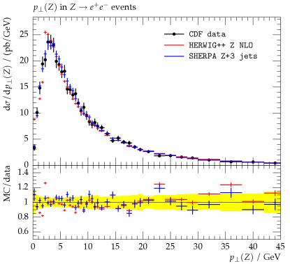
The Z analysis from CDF Run I [7] is a measurement of the cross section as a function of the transverse momentum of pairs in the Z boson mass region of from collisions at = 1.8 TeV, with the measured lepton acceptance extrapolated to with no cut. The analysis is also subject to ambiguities in the experimental Z definition [7].
Fig. 1 shows that the MC description for both Z NLO generation in the formalism and Z+3 jets in the PS+ME formalism agree with CDF data, inside the experimental uncertainties, except for the low Z region for .
D0 Run II results
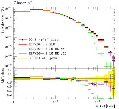
The D0 Z () analysis [8] is based on collisions at = 1.96 TeV, with a looser lepton pair mass cut of GeV. The measured differential spectrum is normalized to the total Z cross section, to reduce overall systematic uncertainties. The electrons were measured in || < 1.1 or 1.5 < || < 2.5, with > 25 GeV. The result was extrapolated to with no cut.
We can see in Fig. 2 (left) that the D0 analysis in the electron Z decay channel has a systematic behaviour in the region of medium Z , for both Z NLO ( formalism), Z LO with ME formalism and Z + 3 jets. The NLO plot shows slightly better behaviour in the mid region (30-60 GeV) than the LO with ME corrections, but no significant differences in the low region. The high region lacks the statistics to make a detailed comparison.
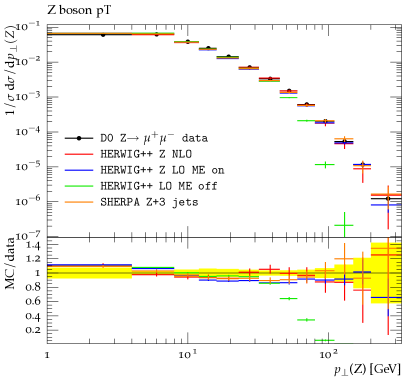
The middle region suggests a problem either with the the Monte Carlo or something in the analysis. We therefore looked also at a new D0 Z analysis [9] in the muon channel. The muons were measured in || < 1.7 and > 15 GeV. This new analysis has as an important development: the definition of the final observable is made at the level of particles entering the detector, while previous measurements have applied theoretical factors correcting for any final state radiation and for the measured lepton acceptance to full coverage. This new approach minimises the dependence on theoretical models, and therefore any biases in comparisons. The differential cross section is normalized to the total Z cross section, to reduce overall systematic uncertainties, as in the electron channel analysis [8].
We can see in Fig. 2 (right) that in the muon channel the discrepancy in the medium Z transverse momentum region is gone, and the ratio of MC to data does not show significant systematic discrepancies for both generators. So the Monte Carlo can better reproduce the analysis with the more limited lepton acceptance and without the model dependent corrections. For LO without ME corrections, the expected behaviour is to produce fewer events in the high transverse momentum region, as this is not fully populated by the PS formalism alone.
4.2.1 PDF and choice on
For the sake of using the best parameters for the description of Tevatron data, some other parameters were studied in the generator: the impact of the use of different PDFs and different values for intrinsic transverse momentum of the partons within the hadrons () and its gaussian width ().
The same Z () analysis [9] of the previous section is used, for the reasons discussed above.
Intrinsic Transverse Momentum of Partons Within the Hadrons
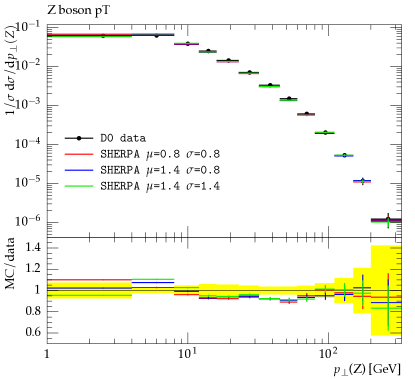
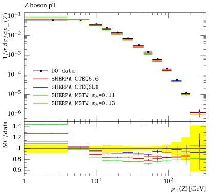
In Fig. 3 (left) we show the transverse momentum of the Z boson in Z+3 jets production with different values for the transverse momentum of the partons within the hadrons. We can see that the = 1.4 (the default value is 0.8) and = 0.8 (default value) shows a better agreement in the lowest Z bin.
PDF Set With Different Values
In order to show the impact of changing the PDF on the shape of the Z , the analysis was run with the [10] set, that is a set of PDFs fitted with different values of the strong coupling constant in the Z mass pole, . Fig. 3 shows the change introduced by varying . These were compared to two other PDFs: the default in , , and to . The last provides a better description of the Z data, especially in the low transverse momentum region. For with , a NLO PDF is necessary, and all the simulations used the default one, [11].
4.3 Multiple Parton Interactions
With both generators providing a reasonable description of the Z , we can study the rest of the event in more detail. However, before looking at the jets recoiling against the Z, we must first constrain the other source of hadronic activity, MPI.
4.3.1 Constraining UE/MPI
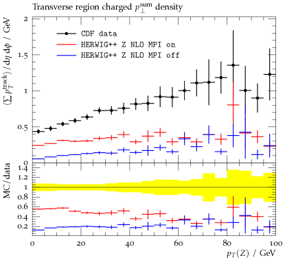
To study the model of the MPI in each of the generators used, the CDF underlying event analysis [12] was compared to both the and generators.
The analysis was made for Drell-Yan events with and . A mass cut GeV was applied at the generator level. The analysis is based on the observation that the hard interaction in an event typically falls along an axis, and activity from MPI is completely uncorrelated with this axis. Each event is therefore decomposed into regions in the azimuthal angle, . The "toward" region defined by the direction of the Z, which is used to set = 0. The opposite direction, the "away" region, is then dominated by the recoil to the Z. The "transverse" regions, defined by 60 < < 120, generally have little activity from the hard interaction, and so are most sensitive to MPI and the underlying event. In the analysis, the transverse region is defined for || < 1 [12].
Fig. 4 shows the comparison of to the CDF data with the MPI model turned on and off. There appears to be a disagreement in the observed UE, with always producing less activity than the data in the transverse region. The default settings for the MPI model in were tuned to provide the best fit to the jet data from Run I and Run II. Adjusting some of these parameters does not yield a significant improvement in the description of the Z data, however [3].
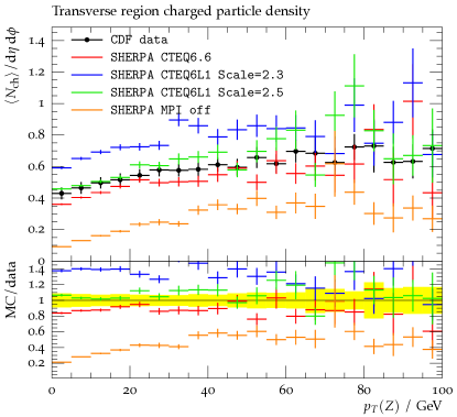
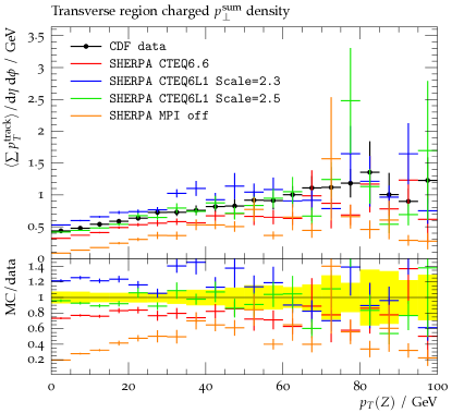
For the generator, comparisons are made with the default settings for MPI [13]. Changing the PDF to , which provided the best description of the Z , significantly degrades the MPI model performance, most probably due to the different value of () and running of between the two PDF sets. The most important parameter in tuning the MPI model is the scale of the transverse momentum cutoff, and three values are tested with the PDF: 2.1, 2.3 and 2.5 GeV. The plots in Fig. 5 show that the best settings for are the PDF with the scale set to 2.5 GeV.

4.4 Z + jets - and LO vs NLO
We now return to our main aim: to assess the impact of NLO matrix elements in the simulation of Z (+ jets) events. We use the following generator configurations: LO without ME correction, LO with ME correction and NLO ( formalism), for the generator; and Z + 3 jets at LO for the generator.
Table 1 shows a comparison of the total Z cross section measured at the Tevatron CDF experiment [14]. As expected, the NLO simulation has the best prediction of the cross section, while at LO, has a slightly better prediction than . Further comparisons between the ME+PS merging in and (besides and ) can be found in reference [15].
| Total [pb] | Uncertainty [pb] | |
|---|---|---|
| CDF data | 256.0 | 2.1 |
| LO ME on | 185.1 | 0.7 |
| LO ME off | 185.2 | 0.7 |
| NLO | 230.4 | 0.9 |
| Z + 1 jet | 171.5 | 0.3 |
| Z + 3 jets | 172.6 | 0.4 |
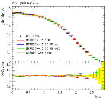
Z boson rapidity
Fig. 6 shows the D0 measurement of the Z cross section as a function of the Z boson rapidity [16]. All generators describe the data well. The differential cross section is also normalized to the total cross section for Z production.
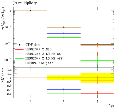
Jet multiplicity
In Fig. 7 (left) the CDF Z [10] analysis shows the cross section as a function of jet multiplicity. The jets are required to have > 30 GeV and to be within the rapidity range, . The plot is then normalized to the cross section of production of Z+1 jet (first bin) in data. This is useful to test the relative fraction of two and three jet events. We can see that the Z+3 jets generator can describe, inside data uncertainties, the expected number of events with two and three jets, while fails for jet multiplicities higher than one.
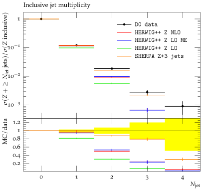
The D0 Z analysis [17] measures the -jet cross section ratios and is shown in Fig. 7 (right). The distribution is inclusive and normalized to the total Z data cross section (i.e., the bin of zero or more jets). Here we can see that the Z NLO , LO with ME corrections and Z + 3 jets predictions describe the first jet bin well. For higher jet multiplicities, the Z + 3 jets generator describes the data better, however it fails for four jets, as one may expect. LO without ME corrections does not describe the data in any bins.
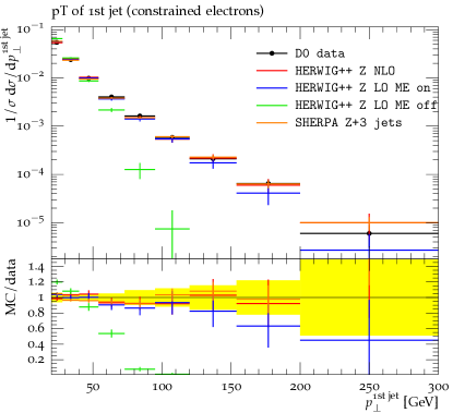
Jet transverse momentum
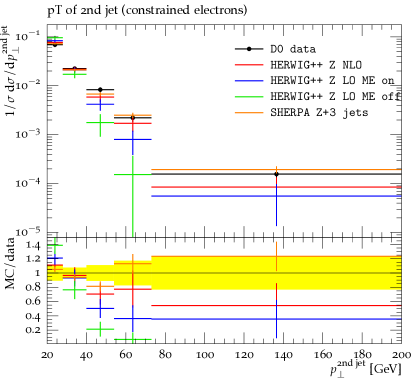
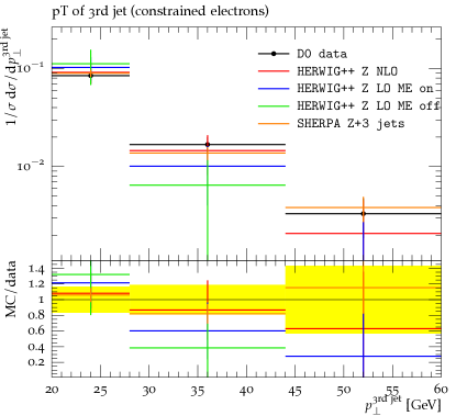
The D0 analysis in [18] measures the differential cross section as a function of the transverse momentum, of the three leading jets in the production of , normalized to the total cross section of production. Fig. 8 shows comparisons with the generator at NLO (POWHEG formalism) and at LO with and without ME corrections, and with Z + 3 jets. The LO without ME corrections shows the expected failure of the parton shower alone to populate the high region, because it corresponds to the phase space where the PS can’t fill properly. When the ME correction is turned on, the effect in correcting the high transverse momentum region can be seen. The behaviour for the NLO plot is more close to the data in the higher region (above 130 GeV), while it has similar results to LO with ME corrections at lower . However, for the second and third leading jets, the description is also not good - NLO Z production includes the LO matrix element for one jet production, but the second and third jets are produced only by the parton shower, which again underestimates the data. For the Z + 3 jets, the matrix element for the further jet emissions allows for a description similar to the NLO curve for the leading jet, and does a better job for the second and third leading jets.
D0 Analysis
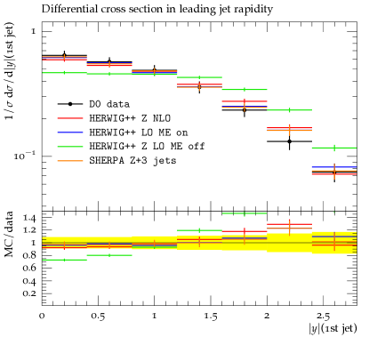
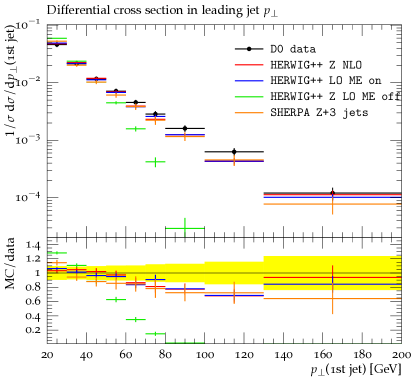
To further study the jet recoil and Z boson , the D0 analysis with Z () + jets [19] was used. It measures the cross sections as a function of the boson momentum, and as a function of momentum and rapidity of the leading jet. It is required at least one jet in the event, with > 20 GeV and < 2.8. This analysis doesn’t normalize the data by the Z total cross section production - the shape of the plots are normalized by their integral.
As can be seen in Fig. 9, the cross section in leading jet rapidity is well behaved inside the uncertainties, however Z LO without ME corrections tends to produce a wider distribution. The Z shows imprecisions in the low momentum region: for Z NLO the production in low Z is around 40% lower than data, and in it’s greater than data. This region is particularly sensitive to jets produced by MPI, which are not recoiling against the Z boson.
The leading jet does not show any significant discrepancy in both cases. However, a behaviour that one can see is the deficit of events in the Monte Carlo compared to the data in the range of 50 < < 120 GeV. The Z shows no such deficit (see Fig. 2), suggesting the MC is not fully describing the hadronic recoil of the Z, and this is studied in detail in the appendix.
LO with ME corrections show similar behaviour to the NLO prediction, and without the ME corrections has a completely different shape in all plots, due to the previously discussed issues in populating the high regions.

5 LHC Analyses Cuts
After choosing the Monte Carlo parameters for the Z NLO (in formalism) and Z + 3 jets (LO), comparison plots for in the LHC energy (first Run - 7 TeV) were performed, using the following kinematic cuts (taken from [20]):
-
•
Transverse momentum of the lepton ;
-
•
Absolute value of the lepton pseudorapidity ;
-
•
Transverse momentum of the jet ;
-
•
Absolute value of the jet pseudorapidity ;
-
•
Lepton isolation criteria: ; ;
The jets are reconstructed with the clustering algorithm, with cone radius R=0.7. A mass cut on the leptons invariant mass was applied. The events generated correspond to a integrated luminosity of 1 .
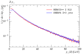
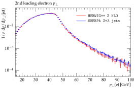
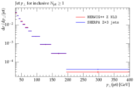
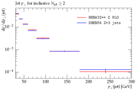
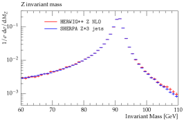
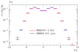
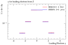
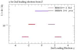
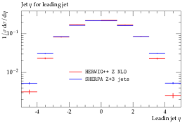
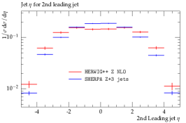
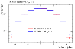
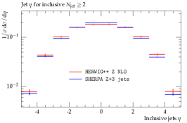
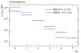
The kinematic variables plotted are shown in Figs. 10 to 15: the transverse momentum of the first, second and third leading jets, and the inclusive for 1 and 2 or more jets in the event; the transverse momentum of the two leptons used to reconstruct the Z boson, and of the Z; The pseudorapidity of Z and jets; the invariant mass of the Z; the jet multiplicity in the event. All the plots are normalized to their integral, except the jet multiplicity, that is the cross section of production of the event with -jets.
The Z (Fig. 10 left) shows a discrepancy in the low transverse momentum region: simulates fewer events in this region, compared to . However, for the leading electrons of the event (Fig. 10 center and right), the discrepancy isn’t as much as for the boson .
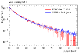
For the leading jet (Fig. 11 left), the behaviour is also discrepant - the generator simulates more events in the low transverse momentum region, and fewer events in medium and high transverse momentum, although in the later ones it agrees with inside the statistical uncertainties. For the second and third leading jets (Fig. 11 center and right), there is good agreement inside MC uncertainties.
The jet for and , that is the transverse momentum of all jets in the event that pass the cuts > 30 GeV and < 2.1 for events with at least one or two jets (Fig. 12 left and center, respectively) agree in both generators inside the errors, as well as the invariant mass of the Z boson (Fig. 12 right).
The pseudorapidity for the Z boson and leading electrons (Fig. 13) agree for the generators, inside the errors. However, for the leading jets, the behaviour is different: while for the leading jet (Fig. 14 left) the region in which < 3 is agreed, the region in the range shows fewer events for the generator than for . For the second leading jet (Fig. 14 center), has more events in the central region and fewer events in the range . For the third leading jet (Fig. 14 right), due to high statistical errors, both generators agree in full range. In the jet inclusive for (Fig. 15 left) the range of shows more events for generator, while for (Fig. 15 center) the generators agree inside errors.
For the cross section as a function of jet multiplicity (Fig. 15 right), the simulation of Z production at NLO ( formalism) has a greater cross section than Z+3 jets at LO for the production of one and two jets. However, because takes into account matrix elements up to 3 jets, the description for higher jet multiplicities have a greater cross section for the generator. The data will usually have greater cross sections than predicted with the generators, because for having equal cross sections one should simulate up to infinite orders of QCD.


6 Conclusions
We studied the effects of adding a next to leading order term in the Monte Carlo simulation for Z production in hadron colliders. In addition, the influence of adding a matrix element correction in the leading order calculations for improving the showering in the parton shower formalism, and the influence of some theoretical parameters that enter as input in the Monte Carlo programs.
We could see that the use of the NLO term, studied here in the formalism as implemented in the generator, improves the prediction of the cross sections of the processes, as well as the behaviour of the physics observables, specially in the region of higher transverse momentum. The implementation of the matrix element correction in the parton shower formalism also improves the description of the data in the region of high transverse momentum, compared to the calculations in leading order without the correction.
It was also seen that both and generators show a systematic behaviour lower than the Tevatron data in the region of mid-range transverse momentum of the Z boson. The D0 analysis performed in the muon channel has a better Monte Carlo description than the one performed in the electron channel, and doesn’t use any kind of extrapolation based in theory. According to the new muon analysis, if the same theory based corrections are applied, the muon data agree with the electron channel data. So, these theoretical dependent corrections could be responsible for the disagreement and the systematic behaviour between the Monte Carlo and the Tevatron data in mid range transverse momentum of the Z.
The underlying event analysis showed that it is possible to choose a good tune for the parameters in the multiple parton interactions model (Amisic) for the generator, using the PDF that best describes the Z data (). However, for the generator, there was no parameter selection that could describe well the underlying event data, and the setup used was the standard one, based in the best description of other physics observables by the authors.
In the analysis of the balance of the Z against the leading jet and the sum of of all jets in the event was possible to see the effects that the MPI model have in the region of low transverse momentum. This is done in the appendix.
The analysis for LHC first run energy (7 TeV) shows that some kinematic quantities have a different prediction from Z NLO when compared to Z+3 jets simulation, such as the low region of the Z boson transverse momentum and leading jet and leading jets pseudorapidity in the high absolute value of range. For the cross section of jet production, the Z NLO generator predicts a higher cross section for the first and second jets, while the Z+3 jets show higher cross sections for higher jet multiplicities. A full comparison once LHC has enough luminosity will show some features that the Monte Carlo generators will have to be able to deal with, implementing in their processes new information that the new data will provide.
Acknowledgements
We would like to thank Frank Siegert, Prof. F. Krauss, Prof. Peter Richardson, for many useful discussions.
This work was supported by the Marie Curie Research Training Network “MCnet” (contract number MRTN-CT-2006-035606).
Appendix
Jet Recoil
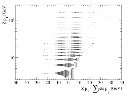
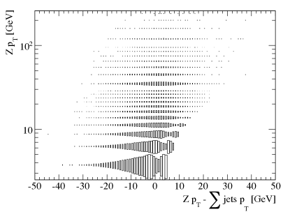
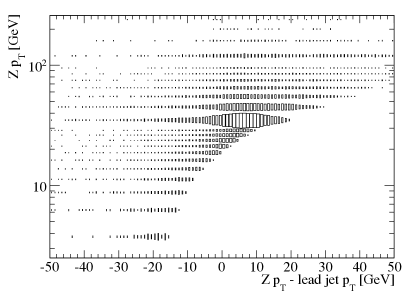
Because primarily the Z should be balanced in the event with the of the leading jet (or all jets in the event), the study of the shape of the jet should give some information about the systematic difference in the description of the , and the leading jet in Z events. With the data, it is impossible to isolate the different effects of MPI and hard scatters, or extend below the cuts used in analysis. So, we perform some studies to check the balance in the MC samples, to see if the Z was summing up to zero when added to the of the leading jet, the sum of the of all jets and, for a more fundamental check of balance, with the sum of the of all particles found in the event.
The first sanity check was done to assure that the sum of the transverse momentum of all particles in the event was balanced, so that both MC generators and were dealing with the events correctly. After this check, the Z balance against the sum of the of all jets in the event and leading jet was analyzed, for both and generators, with multiple parton interactions (MPI) turned on and off.
For the study of the balance of the leading jet, the Tevatron analysis cuts are used ((jet) > 20 GeV and || < 2.1), so it can be comparable to the jet and Z spectra. In the other hand, very loose cuts ((jet) > 5 GeV and || < 10) were applied to analyse the balance of the Z against the sum of all jets in the events, so it’s possible to truly test the balance between jets and Z at generator level.
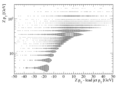
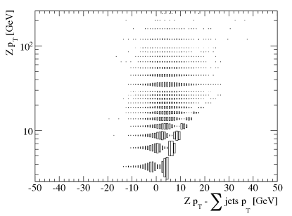
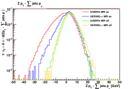
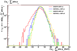
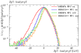
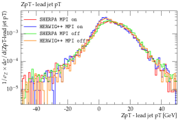
Fig. 16 shows that with the MPI model turned on, the and generators have different behaviour for low Z region: shows more events concentrated in the region of (Z - jets ) = -17 for the leading jet and (Z - jets ) in the range of [-5, 0] for the sum of jets, while shows a behaviour that is very similar to that without the MPI model, in Fig. 17, upper plots.
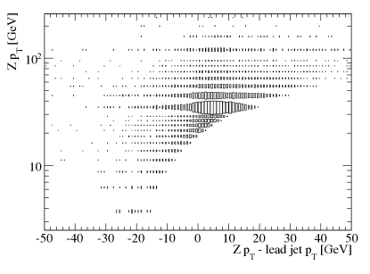
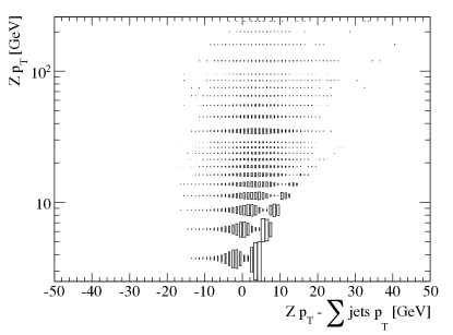
Fig. 17 shows that for the MPI model off in the generators, the behaviour is similar. However in Fig. 16 there is more in the jets, so this isn’t balancing exactly all the transverse momentum that comes from the Z boson. Specially in the low region of the boson , we are probably seeing additional particles from MPI that don’t contribute to the Z but do contribute to the jet .

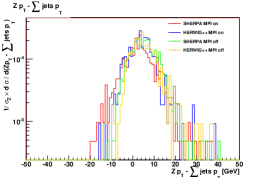
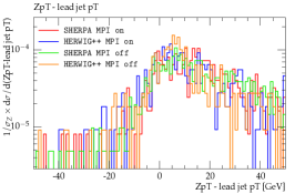
For a better comparison of the plots, we also make one-dimensional projections of the plots for three different Z regions (Z < 30 GeV, 30 GeV < Z < 100 GeV, Z > 100 GeV). These plots (Figs. 18 and 19) make more evident the difference that one can see, specially in the lower region, between the generators with MPI model turned on. and disagree from each other in the balance for both the sum of all jets and leading jet . However, they agree reasonably when there is no simulation of multiple parton interactions. This makes more evident that these models should be better studied and implemented in the context of the Drell Yan production, as have already been shown concerning the generator in the UE analysis.
Leading Jet Rapidity for jet GeV
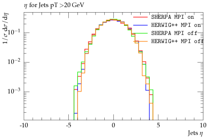
The MPI model in each simulation is clearly producing additional jets in Z events, and we may expect these MPI jets to have a different angular distribution to jets from the hard process. So finally we check the rapidity distribution of all jets with > 5 GeV. It can be seen that, when the MPI are turned on in the simulation, the shape is different in the central region: around the pseudorapidity zero, we have a low bump, when compared to the plots without MPI simulation (Fig. 20 left).
The behaviour is almost gone when the cut on the jets is that of the analysis (Fig. 20 right) - the MPI model affects specially the production of particles in low transverse momentum region. Once more, the MPI model in the generators disagree between themselves. While such a low region is experimentally difficult or impossible to access, it is clearly a very sensitive region for MPI tuning and data with cuts as low as possible are very interesting.

References
- [1] S. Hoeche, F. Krauss, S. Schumann and F. Siegert, “QCD matrix elements and truncated showers,” JHEP 0905 (2009) 053 [arXiv:0903.1219 [hep-ph]].
- [2] T. Gleisberg, S. Hoeche, F. Krauss et al., “Event generation with SHERPA 1.1,” JHEP 0902 (2009) 007. [arXiv:0811.4622 [hep-ph]].
- [3] M. Bahr, S. Gieseke, M. A. Gigg et al., “Herwig++ Physics and Manual,” Eur. Phys. J. C58 (2008) 639-707. [arXiv:0803.0883 [hep-ph]].
- [4] M. H. Seymour, “Matrix element corrections to parton shower algorithms,” Comput. Phys. Commun. 90 (1995) 95-101. [hep-ph/9410414].
- [5] S. Frixione, P. Nason, C. Oleari, “Matching NLO QCD computations with Parton Shower simulations: the POWHEG method,” JHEP 0711 (2007) 070. [arXiv:0709.2092 [hep-ph]].
- [6] A. Buckley, J. Butterworth, L. Lonnblad et al., “Rivet user manual,” [arXiv:1003.0694 [hep-ph]].
- [7] A. A. Affolder et al. [ CDF Collaboration ], “The Transverse momentum and total cross-section of e+ e- pairs in the Z-boson region from p anti-p collisions at S**(1/2) = 1.8-TeV,” Phys. Rev. Lett. 84 (2000) 845-850. [hep-ex/0001021].
- [8] V. M. Abazov et al. [ D0 Collaboration ], “Measurement of the shape of the boson transverse momentum distribution in p anti-p —> Z / gamma* —> e+ e- + X events produced at s**(1/2) = 1.96-TeV,” Phys. Rev. Lett. 100 (2008) 102002. [arXiv:0712.0803 [hep-ex]].
- [9] V. M. Abazov et al. [ D0 Collaboration ], “Measurement of the normalized transverse momentum distribution in collisions at TeV,” Phys. Lett. B693 (2010) 522-530. [arXiv:1006.0618 [hep-ex]].
- [10] A. D. Martin, W. J. Stirling, R. S. Thorne et al., “Parton distributions for the LHC,” Eur. Phys. J. C63 (2009) 189-285. [arXiv:0901.0002 [hep-ph]].
- [11] A. D. Martin, R. G. Roberts, W. J. Stirling et al., “Physical gluons and high E(T) jets,” Phys. Lett. B604 (2004) 61-68. [hep-ph/0410230].
- [12] A. A. Affolder et al. [ CDF Collaboration ], “Charged jet evolution and the underlying event in proton - anti-proton collisions at 1.8-TeV,” Phys. Rev. D65 (2002) 092002.
- [13] T. Sjostrand, M. van Zijl, “A Multiple Interaction Model for the Event Structure in Hadron Collisions,” Phys. Rev. D36 (1987) 2019.
- [14] T. A. Aaltonen et al. [ CDF Collaboration ], “Measurement of of Drell-Yan pairs in the Mass Region from Collisions at TeV,” Phys. Lett. B692 (2010) 232-239. [arXiv:0908.3914 [hep-ex], arXiv:0908.3914 [hep-ex]].
- [15] P. Lenzi, J. M. Butterworth, “A Study on Matrix Element corrections in inclusive Z/ gamma* production at LHC as implemented in PYTHIA, HERWIG, ALPGEN and SHERPA,” [arXiv:0903.3918 [hep-ph]].
- [16] V. M. Abazov et al. [ D0 Collaboration ], “Measurement of the shape of the boson rapidity distribution for p anti-p —> Z/gamma* —> e+ e- + X events produced at s**(1/2) of 1.96-TeV,” Phys. Rev. D76 (2007) 012003. [hep-ex/0702025 [HEP-EX]].
- [17] V. M. Abazov et al. [ D0 Collaboration ], “Measurement of the ratios of the Z/gamma* + >= n jet production cross sections to the total inclusive Z/gamma* cross section in p anti-p collisions at s**(1/2) = 1.96-TeV,” Phys. Lett. B658 (2008) 112-119. [hep-ex/0608052].
- [18] V. M. Abazov et al. [ D0 Collaboration ], “Measurements of differential cross sections of Z/gamma*+jets+X events in proton anti-proton collisions at s**(1/2) = 1.96-TeV,” Phys. Lett. B678 (2009) 45-54. [arXiv:0903.1748 [hep-ex]].
- [19] V. M. Abazov et al. [ D0 Collaboration ], “Measurement of differential Z / gamma* + jet + X cross sections in p anti-p collisions at s**(1/2) = 1.96-TeV,” Phys. Lett. B669 (2008) 278-286. [arXiv:0808.1296 [hep-ex]].
- [20] J. M. Campbell, R. K. Ellis, D. L. Rainwater, “Next-to-leading order QCD predictions for W + 2 jet and Z + 2 jet production at the CERN LHC,” Phys. Rev. D68 (2003) 094021. [hep-ph/0308195].