Multidimensional models of hydrogen and helium emission line profiles for classical T Tauri Stars: method, tests and examples

Abstract

We present multidimensional non-LTE radiative transfer models of hydrogen and helium line profiles formed in the accretion flows and the outflows near the star-disk interaction regions of classical T Tauri stars (CTTSs). The statistical equilibrium calculations, performed under the assumption of the Sobolev approximation using the radiative transfer code torus, has been improved to include He i and He ii energy levels. This allows us to probe the physical conditions of the inner wind of CTTSs by simultaneously modelling the robust wind diagnostic line He i $\lambda 10830$ and the accretion diagnostic lines such as Pa$\beta$, Br$\gamma$ and He i $\lambda 5876$. The code has been tested in one and two dimensional problems, and we have shown that the results are in agreement with established codes. We apply the model to the complex flow geometries of CTTSs. Example model profiles are computed using the combinations of (1) magnetospheric accretion and disc wind, and (2) magnetospheric accretion and the stellar wind. In both cases, the model produces line profiles which are qualitatively similar to those found in observations. Our models are consistent with the scenario in which the narrow blueshifted absorption component of He i $\lambda 10830$ seen in observations is caused by a disc wind, and the wider blueshifted absorption component (the P-Cygni profile) is caused by a bipolar stellar wind. However, we do not have a strong constraint on the relative importance of the wind and the magnetosphere for the ‘emission’ component. Our preliminary calculations suggest that the temperature of the disc wind and stellar winds cannot be much higher than $\sim$10,000 K, on the basis of the strengths of hydrogen lines. Similarly the temperature of the magnetospheric accretion cannot be much higher than $\sim$10,000 K. With these low temperatures, we find that the photoionzation by high energy photons (e.g. X-rays) is necessary to produce He i $\lambda 10830$ in emission and to produce the blueshifted absorption components.

1 Introduction

Mass-loss processes in young stellar objects (YSOs), such as the classical T Tauri stars (CTTSs), are a fundamental problem in the star formation process. The origin and the physical conditions of the wind from YSOs are crucial to our understanding of the protostellar phase and of the evolution of protostellar discs. The mass-loss process is closely related to the evolution of the stellar rotation since it is one of the possible mechanisms through which YSOs may lose their angular momentum (e.g. Hartmann & Stauffer 1989; Matt & Pudritz 2005; 2007a; 2008a). The mass-loss due to winds may solve the so-called ‘angular-momentum problem’, in which a large fraction of accreting CTTS have rather slow rotations (Herbst et al., 2007) at $\sim 10$ per cent of break-up speed (e.g.,  Matt & Pudritz 2007b) despite of a rather large amount of the angular momentum added to stars by accretion process.

Most likely, the outflows are formed in magnetohydrodynamics processes in which a large-scale open magnetic field is anchored to a rotating object; however, whether the object is the disk, central star or both is still unclear (Edwards et al. 2006; Ferreira, Dougados, & Cabrit 2006; Kwan, Edwards, & Fischer 2007). There are at least three possible configurations of the wind formation: (1) a disc wind in which one assumes a sufficient magnetic field and ionization fraction to launch magneto- centrifugal winds over a relatively wide range of disk radii, from an inner truncation radius out to a several au (e.g. Ustyugova et al. 1995; Romanova et al. 1997; Ouyed & Pudritz 1997; Ustyugova et al. 1999; Königl & Pudritz 2000; Krasnopolsky et al. 2003; Pudritz et al. 2007), (2) an X-wind in which the wind launching region is restricted to a narrow region near the inner edge of the accretion disk around the corotation radius where the disk interfaces with the stellar magnetosphere (Shu et al. 1994), and (3) a stellar wind in which outflows occurs along the open magnetic fields from the stellar surface (e.g., Hartmann, Avrett, & Edwards 1982; Kwan & Tademaru 1988; Hirose et al. 1997; Romanova et al. 2005; Cranmer 2009). Interestingly, recent MHD simulations by Romanova et al. (2009) found yet another type outflow called ‘conical winds’ which are produced when the stellar dipole magnetic field is squeezed by the disc into the X-wind type configuration. The resulting outflow occurs in rather narrow conical shapes with their half opening angles between $30^{\circ}$ to $40^{\circ}$. This conical wind is similar to the X-wind mentioned above, but the former is driven by the magnetic force and it does not required to have the magnetospheric radius matched with the corotation radius of the system. More recent simulations performed with larger radial domains have shown that the conical winds become strongly collimated by the magnetic force at larger distances (Lii, Romanova, & Lovelace 2011; Königl, Romanova, & Lovelace 2011).

In order to distinguish between the different theoretical models, and to understand the origin of the angular momentum transfer, constraints on the wind launching location are very important. Spectroscopic studies of strong emission lines in CTTSs may help to solve this problem. The observations by e.g. Takami et al. (2002), Edwards et al. (2003), Dupree et al. (2005) and Edwards et al. (2006) demonstrated a robustness of optically thick He i $\lambda 10830$ as a diagnostic of the inner wind from the accreting stars. Unlike other strong emission lines (e.g. H$\alpha$ and H$\beta$) which also often show a sign of the inner winds, He i $\lambda 10830$ from CTTS shows P-Cygni type profile (with deep blueshifted absorption below continuum level) which resembles that of the hot stellar winds expanding in radial direction (e.g., Kwan et al. 2007). Edwards et al. (2006) showed that about 70 per cent of CTTS exhibit a blueshifted absorption (below continuum) in contrast to H$\alpha$ which shows about only 10 per cent of stars show similar type of absorption component (e.g., Reipurth, Pedrosa, & Lago 1996). Edwards (2007) and Kwan et al. (2007) suggested that the blueshifted absorption component in the He i $\lambda 10830$ profiles is cased by a stellar wind in about 40 per cent, and by a disc wind in about 30 per cent of the samples in Edwards et al. (2006). Recent local excitation calculations of Kwan & Fischer (2011) in combination with the spectroscopic observations demonstrated the effectiveness of He i $\lambda 10830$ for probing the density and temperature of the inner wind.

In our previous radiative transfer models, (Harries 2000; Kurosawa et al. 2004; Symington, Harries, & Kurosawa 2005; Kurosawa, Harries, & Symington 2006; Kurosawa, Romanova, & Harries 2008), we have considered the statistical equilibrium of hydrogen atoms only. In light of the recent recognition of He i $\lambda 10830$ line as a useful wind diagnostic tool (e.g. Edwards et al. 2006; Kwan et al. 2007; Kwan & Fischer 2011), we improve our model to include helium ions (He i, He ii and He iii). This will allow as to investigate the physical conditions (e.g. geometry, temperature, density and kinematics) of the innermost part of the wind more effectively, and will be a significant improvement to the wind study of Kurosawa et al. (2006) who used only H$\alpha$. If we are to reliably determine mass loss rates and mass accretion rates of CTTSs, a more self-consistent modelling approach is required. This includes a multiple line fitting of observations including both hydrogen and helium to model the wind and magnetospheric accretion flows simultaneously.

Our main goals in this paper are to present the methods and tests for our improved radiative transfer code, and to demonstrate the capability of the code in the applications to the wind and magnetospheric accretion problems of CTTSs. Detailed investigations of the wind and accretions flows, e.g. constraining flow geometry, density, temperature and relative strength of the mass-loss to mass-accretion rates, will be presented in a future paper as these require a large parameter space survey.

In Section 2, the model assumption, the method of statistical equilibrium and the observed profile calculations are presented. The tests of the code in one and two dimensional (1D and 2D respectively) geometries will be given in Section 3. Simple kinematic models of a disc wind and a stellar wind in combinations with a magnetospheric accretion model will be presented in Section 4. Example profiles of hydrogen and helium are also given in the same section. Finally main findings and conclusions are given in Section 6.

2 Radiative transfer code

The radiative transfer code torus (Harries 2000; Kurosawa et al. 2004; Symington et al. 2005; Kurosawa et al. 2006; Kurosawa et al. 2008, but see also Acreman, Harries, & Rundle 2010; Rundle et al. 2010) is extended to include helium ions (He i, He ii and He iii). Our model uses the three-dimensional (3D) adaptive mesh refinement (AMR) grid, and it allows us an accurate mapping of an MHD simulation data on to the radiative transfer grid (without a loss of resolution). The code also works in 2D (axisymmetric) and 1D (spherically symmetric) cases. The basic steps for computing the line profiles are as follows: (1) mapping of the density, velocity and temperature, from either an MHD simulation output or an analytical model, to the radiative transfer grid, (2) the source function ($S_{\nu}$) calculation and (3) the observed flux/profile calculation. In the second step, we adopt the method described by Klein & Castor (1978) (see also Rybicki & Hummer 1978; Hartmann, Hewett, & Calvet 1994) in which the Sobolev approximation method is used. The Sobolev approximation, is valid when (1) a large velocity gradient is present in the gas flow, and (2) the intrinsic line width is negligible compared to the Doppler broadening of the line. In the following, we describe each step of the line profile computation in more detail.

2.1 Grid construction

Our radiative transfer code has been developed to handle length scales in many order of magnitudes and multi-dimensional problems without a particular symmetry (e.g., Kurosawa & Hillier 2001; Symington et al. 2005; Harries et al. 2004; Kurosawa et al. 2004). When the gradient or dynamical range of physical quantities such as density is very large, a logarithmic scale in the radial direction could be used to increase an accuracy of optical depth calculations if the system is spherically or axially symmetric. When a problem requires an arbitrary geometry, there is no simple way to construct a logarithmic scale. However, an efficient cubic or square grid (depending on the problem is 3D or 2D) can be constructed by subdividing a cube/square into smaller cubes/squares where the value of density or opacity is larger than a given threshold value. We use the 8-way/4-way tree (octal/quad tree) data structure to construct the grids and to store the physical quantities required in the radiative transfer calculations. The data structure used here is similar to a binary tree in which one node splits into two child nodes, but ours splits into eight (for 3D) or four (for 2D).

The algorithm used to construct the grid in this paper is very similar to that used in Kurosawa & Hillier (2001). Starting from a large cubic/square cell (with size $D$) which contains a whole computational domain, we first compute the average density of the cell by randomly choosing 100–1000 points in the cell and evaluating the density at each point. The average density is then multiplied by the volume of the cell ($D^{3}$) to find the total mass ($M_{\mathrm{cell}}$) in the cell. If the mass is larger than a threshold mass ($M_{\mathrm{th}}$), which is a user defined parameter, this cell is split into 8 or 4 subcells with size $D/2$. If the mass of the cell is less than the threshold, it will not be subdivided. The same procedure is applied to all the subcells recursively, until all the cells contain a mass less than the threshold ($M_{\mathrm{cell}}<M_{\mathrm{th}}$). Alternatively, if the opacity of the field is known prior to the construction of the grid (which is usually not the case), one can use the optical depth across a cell ($\tau_{\mathrm{cell}}$) and use the condition, $\tau_{\mathrm{cell}}<\tau_{\mathrm{th}}$ where $\tau_{\mathrm{th}}\approx 0.1$, as a condition for cell splitting. More complex algorithms could be used to optimise the computation for a specific problem. Once the data structure is built, the access/search for a given cell can be done recursively, resulting a faster code. Fig. 1 shows an example of the AMR grid constructed for the axisymmetric (dipolar) magnetospheric accretion columns from Hartmann et al. (1994).

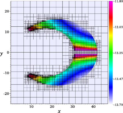
Figure 1: An example of the 2D AMR grid constructed for the density from the magnetospheric accretion model described by Hartmann et al. (1994). The grid structure is overlaid on the colour map of the input density. The density map are logarithmically scaled and in cgs units. The axes are in $10^{10}$ cm. Although not shown here, the accreting star is located at ($x$, $y$) = ($0$, $0$), and its radius is $1.4\times 10^{11}$ cm.

2.2 Statistical equilibrium

Our statistical equilibrium computation essentially follows the method described by Klein & Castor (1978) (hereafter KC78; see also Rybicki & Hummer 1978; Hartmann et al. 1994) who uses the Sobolev approximation. A main difference between the model of KC78 and ours is in the atomic model. Our atomic model consists of 20 bound levels for H i and the continuum level for H ii, 19 levels for He i (up to the principal quantum number $n=4$ level), 10 levels for He ii and the continuum level for He iii. The atomic data used for hydrogen are same as in Harries (2000) and Symington et al. (2005), and those for helium ions are adopted from Hillier & Miller (1998). Here, we have a rather small set of ions and levels; however, the method which are to be described next is not limited to these ions.

Since we intend to apply our model to multi-dimensional problems (2D and 3D), the main limiting factor of the size of the atomic model is computer memory, and CPU time. For example, our typical 2D model with CTTS accretion funnels and wind requires about $2\times 10^{4}$ grid points ($\sim 141^{2}$) and about $300$ Mb of RAM; hence adding more complicated atoms and levels will be not feasible without a major modification to the code. Note that our code is parallelised under Message Passing Interface (MPI), but the domain decomposition of the computational grid has not been implemented because the code is optimised for speed. Adding more ions and modification of the code to handle a grid with domain decomposition will be done in the future.

In the original model of KC78, a simpler atomic model was used. They assumed that a majority of the helium atoms were ionized, and excluded He i levels in their calculation. Their assumption is acceptable since their objective is to model emission lines in the hot wind of Of stars which have $T_{\mathrm{eff}}\gtrsim$30,000 K. The same assumption can not be applied to flows with much lower temperatures such as in the CTTS accretion flows and wind; hence, we have added those extra levels.

In the following, we summarise our computational steps. The following equation of statistical equilibrium is applied to each levels of H i, He i and He ii. The total rates for $j$-th level can be written as:

$$R_{j}^{L}-R_{j}^{U}+R_{j}^{R}-R_{j}^{I}=0,$$ (1)

where $R_{j}^{L}$ is the net transition rate between $j$-th level and the lower bound levels, and similarly $R_{j}^{U}$ is the net transition rate between $j$-th level and the upper bound levels. The last two terms, $R_{j}^{R}$ and $R_{j}^{I}$, are the net recombination and the ionization rates, respectively. The rates in equation (1) are:

$$R_{j}^{L} = \sum_{i<j}\left[n_{i}\left(B_{ij}\mathcal{J}_{ij}+n_{e}C_{ij}\right)\right.$$ (2)

$$\left.-n_{j}\left(A_{ji}+B_{ji}\mathcal{J}_{ij}+n_{e}C_{ji}\right)\right]\,,$$

$$R_{j}^{U} = \sum_{i>j}\Bigl{[}n_{i}\left(A_{ij}+B_{ij}\mathcal{J}_{ij}+n_{e}C_{ij}\right)$$ (3)

$$-n_{j}\left(B_{ji}\mathcal{J}_{ij}+n_{e}C_{ji}\right)\Bigr{]}\,,$$

$$R_{j}^{R} = n_{k}\left(\frac{n_{j}^{*}}{n_{k}^{*}}\right)\Bigl{[}4\pi\int_{\nu_{j}}^{\infty}\frac{a_{j}\left(\nu\right)}{h\nu}\left(\frac{2h\nu^{3}}{c^{2}}+J_{\nu}\right)$$ (4)

$$\times\exp\left(-\frac{h\nu}{kT}\right)d\nu+n_{e}C_{jk}\Bigr{]}\,,$$

and

$$R_{j}^{I}=n_{j}\left(4\pi\int_{\nu_{j}}^{\infty}\frac{a_{j}\left(\nu\right)}{h\nu}J_{\nu}d\nu+n_{e}C_{jk}\right),$$ (5)

where $A_{ij}$ and $B_{ij}$ are the Einstein coefficients between levels $i$ and $j$, and $C_{ij}$ is the collisional rate coefficient. The first and the second subscripts in $A$, $B$ and $C$ correspond to the initial and the final state of a transition, respectively. The subscript $k$ denotes the continuum state. The LTE and non-LTE populations of $i$-th level are written as $n_{i}^{*}$ and $n_{i}$, respectively. While $a_{j}\left(\nu\right)$ is the photoionization cross section of $i$-th level, $J_{\nu}$ is the mean (angle averaged) intensity of the continuum radiation. The symbol $\mathcal{J}_{ij}$ refers to the angle and line profile averaged intensity of the line transition between levels $i$ and $j$ (cf. Mihalas 1978). The electron number density and temperature are specified as $n_{e}$ and $T$. Other symbols have usual meaning. Using the Sobolev approximation (the escape probability theory), $\mathcal{J}_{ij}$, for the transitions with $i<j$, can be simplified as (see e.g. Castor 1970):

$$\mathcal{J}_{ij}=\left(1-\beta_{ij}\right)\frac{2h\nu_{ij}^{3}}{c^{2}}\left(\frac{g_{j}}{g_{i}}\frac{n_{j}}{n_{i}}-1\right)^{-1}+\beta_{c,ij}I_{c,ij},$$ (6)

where $I_{c,ij}$ is the intensity of the continuum around the line frequency $\nu_{ij}$. The symbols $g_{i}$ and $g_{j}$ denote the degeneracy (statistical weight) of the energy levels. Here, we assume that the ‘continuum emissivity and opacity of the gas are very small, and the photospheric photons are unaffected by continuum processes. In equation (6), we neglect the contribution from the non-local emission which are included in the models of Hartmann et al. (1994) and Muzerolle et al. (2001). The effect of this omission is very small as we will see later in Section 3.2. The escape probabilities $\beta_{ij}$ and $\beta_{c,ij}$ in equation (6) are (c.f. Castor 1970; Rybicki & Hummer 1978):

$$\beta_{ij}=\frac{1}{4\pi}\oint\frac{1-e^{-\tau_{ij}}}{\tau_{ij}}d\Omega,$$ (7)

and

$$\beta_{c,ij}=\int_{\Omega_{*}}\frac{1-e^{-\tau_{ij}}}{\tau_{ij}}d\Omega$$ (8)

respectively. In equation (8), the integration is performed over the solid angle of stellar photosphere ($\Omega_{*}$) as seen from the location where $\beta_{c,ij}$ is evaluated. The optical depth $\tau_{ij}$ is defined as

$$\tau_{ij}=c\frac{\chi_{ij}}{\nu_{ij}}\left|\frac{dv_{n}}{dl_{n}}\right|^{-1}.$$ (9)

Here, $dv_{n}/dl_{n}$ is the derivative of the velocity field projected in the direction $\hat{\boldsymbol{n}}$, i.e. $v_{n}=\boldsymbol{v}\cdot\hat{\boldsymbol{n}}$, and $dl_{n}$ is the line element in the direction of $\hat{\boldsymbol{n}}$. The line opacity $\chi_{ij}$ is:

$$\chi_{ij}=\frac{\pi e^{2}f_{ij}n_{j}}{m_{e}c}\left(1-\frac{g_{j}n_{i}}{g_{i}n_{j}}\right),$$ (10)

where $f_{ij}$ is the oscillator strength.

Since we assume that the gas is optically thin to the photospheric continuum radiation, the following simplifications are used for the continuum intensity in equation (6) and the mean intensity in equations (4) and (5). We use the plane-parallel model atmosphere (the Eddington flux $H_{\nu}$) of Kurucz (1979), then they become:

$$I_{c,ij}=4H_{\nu_{ij}}$$ (11)

and

$$J_{\nu}=4WH_{\nu},$$ (12)

where $W$ is the geometrical dilution factor $W=[1-\left(1-R_{*}^{2}/r^{2}\right)^{1/2}]/2$ (cf. Mihalas 1978). Alternatively, we can assume that the photosphere is a blackbody (as in Hartmann et al. 1994; Muzerolle et al. 2001), then we simply have $I_{c,ij}=B_{\nu}\left(T\right)$ and $J_{\nu}=WB_{\nu}\left(T\right)$ with an appropriate photospheric temperature $T$.

The hydrogen particle number conservation gives

$$\sum_{i=1}^{N_{\mathrm{HI}}}n_{i}\left(\mathrm{H\,I}\right)+n\left(\mathrm{H\,II}\right)=\frac{\rho\,X}{\left(X+4Y\right)m_{p}},$$ (13)

where $X$ and $Y$ are the abundances of hydrogen and helium (by number), and $m_{p}$ is the proton mass. The symbol $N_{\mathrm{HI}}$ denotes the number of H i levels (20). Similarly, the helium particle number conservation gives

$$\sum_{i=1}^{N_{\mathrm{HeI}}}n_{i}\left(\mathrm{He\,I}\right)+\sum_{i=1}^{N_{\mathrm{HeII}}}n_{i}\left(\mathrm{He\,II}\right)+n\left(\mathrm{He\,III}\right)$$

$$=\frac{\rho\,Y}{\left(X+4Y\right)m_{p}},$$ (14)

where the numbers of energy levels used here are $N_{\mathrm{HeI}}=19$ and $N_{\mathrm{HeII}}=10$. Unless specified otherwise, we use $X=0.9$ and $Y=0.1$ for the abundances. Finally, the charge conservation gives

$$n\left(\mathrm{H\,II}\right)+\sum_{i=1}^{N_{\mathrm{HeII}}}n_{i}\left(\mathrm{He\,II}\right)+2n\left(\mathrm{He\,III}\right)=n_{e}\,\,.$$ (15)

Equations (1), (13), (14) and (15) form a set of algebraic equations ($N_{\mathrm{HI}}+N_{\mathrm{HeI}}+N_{\mathrm{HeII}}+3$ equations) which contain $N_{\mathrm{HI}}+N_{\mathrm{HeI}}+N_{\mathrm{HeII}}+3$ unknowns. The unknowns here are the level populations of H i, He i, He ii respectively, and the last 3 unknowns are the continuum levels and the electron density, i.e. $n\left(\mathrm{H\,II}\right),$ $n\left(\mathrm{He\,III}\right)$ and $n_{e}$. The set of non-linear algebraic equations will be solved by using the Newton-Raphson iteration method. As a starting point on the iteration, we use either (1) a LTE population or (2) a set of non-LTE solutions from a nearby point which had converged prior to the current computation. The level populations normally converge within 30 iterations.

As mentioned earlier, in our models presented here, the gas temperature $T$ is given as an input because the exact physical processes that determine the plasma temperature of the accretion flow and outflow around CTTS (within a few stellar radii) are not well understood. We therefore hold the temperatures fixed and do not solve the equation of radiative equilibrium.

2.3 Observed profile calculations

The method for the profile calculation is essentially the same as in Kurosawa et al. (2006). Here, we briefly summarise the steps. Once the level populations of H and He are obtained (as in Section 2.2), the emissivity and opacities for the continuum and line ($\eta_{c}$, $\chi_{c}$, $\eta_{l}$ and $\chi_{l}$) can be readily obtained (e.g. equation 10). By following Mihalas (1978), the total source function ($S_{\nu}$) can be written in terms of the continuum and line source function which are defined as $S_{c}\equiv\eta_{c}/\chi_{c}$ and $S_{l}=\eta_{l}/\chi_{l}$, respectively, i.e.

$$S_{\nu}=\frac{\phi_{\nu}S_{l}+h\,S_{c}}{\phi_{\nu}+h},$$ (16)

where $h=\chi_{c}/\chi_{l}$ and $\phi_{\nu}$ is a normalized line profile. When a line broadening is negligible $\phi_{\nu}$ is a normal Doppler profile. However, as noted and demonstrated by Muzerolle et al. (2001) and Kurosawa et al. (2006), with a moderate mass-accretion rate ($~{}10^{-7}\,\mathrm{M_{\sun}\,yr^{-1}}$) of a CTTS, Stark broadening becomes important in the optically thick lines, e.g. in H$\alpha$ and possibly in He i $\lambda 10830$. For those lines, we adopt a Voigt profile to include the broadening effect. The normalized Voigt profile is written as $\phi_{\nu}=\pi^{-1/2}\,H\left(a,y\right)$ where

$$H\left(a,y\right)\equiv\frac{a}{\pi}\int_{-\infty}^{\infty}\frac{e^{-y^{\prime 2}}}{\left(y-y^{\prime}\right)^{2}+a^{2}}\,dy^{\prime}\,\,.$$ (17)

In the expression above, $a=\Gamma/4\pi\Delta\nu_{\mathrm{D}}$, $y=\left(\nu-\nu_{0}\right)/\Delta\nu_{\mathrm{D}}$, and $y^{\prime}=\left(\nu^{\prime}-\nu_{0}\right)/\Delta\nu_{\mathrm{D}}$ (c.f. Mihalas 1978). $\nu_{0}$ is the line centre frequency, and $\Delta\nu_{\mathrm{D}}$ is the Doppler line width of an atom (due to its thermal motion) which is given by $\Delta\nu_{\mathrm{D}}=\left(2kT/m_{\mathrm{i}}\right)^{1/2}\times\left(\nu_{0}/c\right)$ where $m_{\mathrm{i}}$ is either the mass of a hydrogen atom ($m_{\mathrm{H}}$) or that of a helium atom ($m_{\mathrm{He}}$). The damping constant $\Gamma$, which depends on the physical condition of the gas, is parametrised by Luttermoser & Johnson (1992) as follows:

$$\Gamma = C_{\mathrm{rad}}+C_{\mathrm{vdW}}\left(\frac{n_{\mathrm{HI}}}{10^{16}\,\mathrm{cm^{-3}}}\right)\left(\frac{T}{5,000\,\mathrm{K}}\right)^{0.3}$$ (18)

$$+\,C_{\mathrm{Stark}}\left(\frac{n_{e}}{10^{12}\,\mathrm{cm^{-3}}}\right)\,,$$

where $n_{\mathrm{H\,I}}$ and $n_{e}$ are the number density of neutral hydrogen atoms and that of free electrons. Also, $C_{\mathrm{rad}}$, $C_{\mathrm{vdW}}$ and $C_{\mathrm{Stark}}$ are natural broadening, van der Waals broadening, and linear Stark broadening constants respectively. We adopt this parametrisation along with the values of broadening constants from Luttermoser & Johnson (1992). For example, $C_{\mathrm{rad}}=8.2\times 10^{-3}$ Å, $C_{\mathrm{vdW}}=5.5\times 10^{-3}$ Å  and $C_{\mathrm{Stark}}=1.47\times 10^{-2}$ Å for H$\alpha$.

To find an observed line profile, we compute the flux as a function of frequency. The integration of the flux is performed in the cylindrical coordinate system $\left(p,\,q,\,t\right)$ which is obtained by rotating the original stellar coordinate system $\left(\rho,\,\phi,\,z\right)$ so that the $t$-axis coincides with the line of sight of an observer. The observed flux ($F_{\nu}$) is then given by:

$$F_{\nu}=\frac{1}{4\pi d^{2}}\int_{0}^{p_{\mathrm{max}}}\int_{0}^{2\pi}p\,\sin q\,I_{\nu}\,dq\,dp$$ (19)

where $d$, $p_{\mathrm{max}}$, and $I_{\nu}$ are the distance to an observer, the maximum extent to the model space in the projected (rotated) plane, and the specific intensity ($I_{\nu}$) in the direction on observer at the outer boundary. For a given ray along $t$ or alternatively using the optical depth ($\tau_{\nu}$ defined later in equation 21) as an integration variable, the specific intensity is given by:

$$I_{\nu}=I_{0}\,e^{-\tau_{\infty}}+\int_{0}^{\tau_{\infty}}S_{\nu}\left(\tau_{\nu}^{\prime}\right)\,e^{-\tau_{\nu}^{\prime}}\,d\tau_{\nu}^{\prime}$$ (20)

where $I_{0}$ and $S_{\nu}$ are the intensity at the boundary and the source function (equation 16) of the stellar atmosphere/wind at a frequency $\nu$. The upper integration limit $\tau_{\infty}$ is the total optical depth between an observer and the initial integration point. For a ray which intersects with the stellar core, $I_{0}$ is computed from the stellar atmosphere model of Kurucz (1979) (cf. Section 4.1.1), and $I_{0}=0$ otherwise. If the ray intersects with the hot ring on the stellar surface created by the accretion stream, we set $I_{0}=B_{\nu}\left(T_{\mathrm{ring}}\right)$ where $B_{\nu}$ is the Planck function and $T_{\mathrm{ring}}$ is the temperature of the hot ring. The initial position of each ray is assigned to be at the centre of the surface element ($dA=p\,\sin q\,dq\,dp$). We numerically integrate equation (19). A linearly spaced radial grid is used for the area where the ray intersects with magnetosphere, and a logarithmically spaced grid is used for the wind and the accretion disc regions. The numbers of grid points used for a typical integration are $n_{p}=180$, $n_{q}=100$, and $n_{\nu}=101$. The optical depth $\tau_{\nu}$ in equation 20 is defined as:

$$\tau_{\nu}\left(t\right)\equiv\int_{t}^{t_{\infty}}\chi_{\nu}\left(t^{\prime}\right)\,dt^{\prime}$$ (21)

where $\chi_{\nu}$ is the opacity of media, and $t_{\infty}$ is the total distance between the initial integration point and the observer (or to the outer boundary closer to the observer). Equation (21) is also numerically integrated by using the intersection points of a line along $t$ and the AMR grid cells, in which opacities values ($\chi_{\nu}$) are stored. For a high optical depth, additional points are inserted between the original points along the line, and emissivity and opacity are interpolated to those points to ensure $d\tau_{\nu}<0.05$ for the all line segments.

3 Code tests

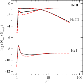
Figure 2: Left panel: The density (top), temperature (middle) and radial velocity (bottom) of the hot stellar wind model of AV 83 computed by cmfgen. The values are shown as a function of radius $r^{\prime}$, which is in the unit of stellar radius (19.6 $\mathrm{R_{\sun}}$). The same density, temperature and velocity distributions are used in torus for the calculation of the statistical equilibrium. Right panel: Comparison of the number fractions of helium ions as a function of radius, computed by cmfgen (solid) and torus (dashed). The fractions here are defined as $N_{\mathrm{ion}}/N_{\mathrm{total}}$ where $N_{\mathrm{ion}}$ is the number density of helium ions (He i, He ii or He iii), and $N_{\mathrm{total}}$ is the total number density of ions, including both hydrogen and helium. The fraction of He i is much smaller compared to those of He ii and He iii. Overall agreements of the two codes are very good.

3.1 1D test : comparison with cmfgen model of Hillier & Miller (1998)

We first test the validity of our statistical equilibrium calculation and the observed profile calculations in a simple geometry. For this purpose, we consider a case of spherical stellar wind from an Of supergiant star since it often exhibits hydrogen and helium in emission. A detail atmosphere model of AV 83 (an O7 Iaf+ supergiant) in the Small Magellanic Cloud (SMC) has been presented by Hillier et al. (2003). Their models are computed by the non-LTE line-blanketed atmosphere code cmfgen (Hillier & Miller 1998) in which the level populations are solved in the co-moving frame and in a spherical geometry. This code has been well-tested and used in numerous investigations of stellar winds of massive stars (e.g. Hillier & Miller 1999; Crowther et al. 1999; De Marco et al. 2000; Dessart et al. 2000; Herald et al. 2001; Martins, Schaerer, & Hillier 2005; Hillier et al. 2006). AV 83 is one of two O stars in the SMC which shows a normal Of spectrum (c.f. Walborn et al. 1995; Walborn et al. 2000). It has a relatively dense stellar wind, and consequently exhibits many wind features in their spectrum. The model presented by Hillier et al. (2003) suggests that AV 83 has the effective temperature of $\sim$32,800 K and the mass-loss rate of $7.3\times 10^{-7}\,\mathrm{M_{\sun}\,yr^{-1}}$.

In the following, we compare the results of the statistical equilibrium calculations and the line profiles computed by torus and cmfgen. Both models assume the hydrogen and helium abundances $X=0.834$ and $Y=0.167$ (by numbers), respectively. To match the same physical conditions in the stellar wind structure, torus adopts the temperature, density and velocity of the wind used in cmfgen, which are shown in Fig. 2. We also adopt the continuum flux from cmfgen in computing the radiation fields in equations 11 and 12. Further, we consider the case without the wind clumping, i.e. a smooth stellar wind case. The cmfgen model data of AV 83 used here for comparison are available on the web site with the address: http://kookaburra.phyast.pitt.edu/hillier/web/CMFGEN.htm.

Since our code torus has newly adopted helium ions in the statistical equilibrium calculation, here we concentrate on the comparisons of the helium calculations. The hydrogen level population calculations had been already tested elsewhere (Harries 1995; Harries 2000; Symington et al. 2005). Fig. 2 shows the number fractions of helium ions in three stages (He i, He ii and He iii) as a function of radial distance from the centre of the star ($r^{\prime}$). The dominating ions of helium are He ii and He iii, and the number fraction of He i typically $\sim 10^{4}$ to $\sim 10^{5}$ times smaller than those of other ions. The figure shows the agreement of the ion fractions computed by both codes is good at all radii, except at $r^{\prime}\sim 2$ (measured in stellar radius) where He i and He ii fractions of torus are smaller than those of cmfgen by a factor of a few.

As one can see in Fig. 2, in this particular model of AV 83, He ii is the most abundant ion up to a several radii. Correspondingly the optical thickness of the continuum photon beyond the He ii Lyman continuum is expected to be very high. This contradicts with our assumption made in Section 2.2 which stated that the gas is optically thin to the photospheric continuum radiation. Therefore, when the He ii Lyman continuum is optically thick, we introduce the following special treatment in the statistical equilibrium. We assume that the radiation field beyond the He ii Lyman edge will be reduced to the local source function, and there is radiative detail balance in the He ii Lyman continuum. In practice, we simply set the photorecombination and photoionization terms in equations 4 and 5 for the ground state of He i to negligibly small values. The atmosphere is still assumed to be optically thin to continuum in all other wavelengths. The same special treatment of the He ii Lyman continuum was used by KC78 who modelled the winds from Of stars. Without this treatment, our ionization fraction of helium ions will be very different from those of the cmfgen model at small radii (e.g.  $r^{\prime}<2$) .

Fig. 3 compares the line emissivity and opacity of He i $\lambda$10830 computed by torus and cmfgen as a function of radius. As mentioned earlier, this particular line has been identified as one of the important wind diagnostic lines in CTTSs (e.g. Edwards et al. 2006; Kwan et al. 2007). The figure also shows the electron scattering opacity, and the continuum opacity and emissivity at the line centre of He i $\lambda$10830. Overall agreement between the two codes is excellent for the continuum emissivity and opacities at all radii. The agreements are also good in the line opacity and emissivity except for the line emissivity ($\eta_{\mathrm{L}}$) at the inner most radii ($r^{\prime}<1.1$) where the outflow speed is subsonic; hence, the Sobolev approximation is not suitable there. The figure also shows the corresponding optical depth ($\tau_{L}$) evaluated at the line centre of He i $\lambda$10830.

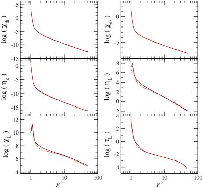
Figure 3: Comparison of opacities, emissivities and optical depth as a function of radius, computed by cmfgen (solid) and torus (dashed). The line opacity ($\chi_{\mathrm{L}}$) and emissivity ($\eta_{\mathrm{L}}$) are those of He i $\lambda$10830. The continuum emissivity ($\eta_{\mathrm{c}}$) and the thermal opacity ($\chi_{\mathrm{th}}$) are evaluated at the line frequency of He i $\lambda$10830. The electron scattering opacity is shown as $\chi_{\mathrm{es}}$. The opacities and emissivities shown are in arbitrary units. The optical depth ($\tau_{L}$) is evaluated at the line centre of He i $\lambda$10830, and it is the sum of the line and continuum optical depths. The radius ($r^{\prime}$) is in the unit of stellar radius which is 19.6 $\mathrm{R_{\sun}}$. The agreements between the two codes are excellent for the continuum emissivity and opacities at all radii. The agreements are also good in the line opacity and emissivity except for those at the inner most radii ($r^{\prime}<1.1$) where the optical depth is very high and the outflow speed is subsonic.

Using the opacities and emissivities above, we now compute the line profiles as seen by an observer. Fig. 4 shows the normalized profile of He i $\lambda$10830 and H$\alpha$ computed by torus and cmfgen. For a simplicity, the broadening effects such as the Stark broadening and rotational broadening are not included in these calculations. He i $\lambda$10830 shows a narrow emission near the line centre and a shallow but very wide wind absorption in the blue side. On the other hand, H$\alpha$ profiles show a wider emission and a relatively narrow wind absorption in the blue. The extent of the red wings in the He i $\lambda$10830 and H$\alpha$ lines is similar, and they both reach the velocity $\sim 800\,\mathrm{km~{}s^{-1}}$ which is very similar to the terminal velocity of the stellar wind ($900\,\mathrm{km~{}s^{-1}}$) used in the models. The figure shows the emission components of both H$\alpha$ and He i $\lambda$10830 profiles computed by torus are slightly stronger than those by cmfgen; however, overall agreement of the line profiles with those of cmfgen is very good.

Figure 4: Comparison of line profiles (He i $\lambda 10830$: right panel and H$\alpha$: left panel) computed by cmfgen (solid) and torus (dashed). The line strengths of the profiles computed by torus are slightly stronger than those of cmfgen; however, overall agreement of the models is excellent. In both lines, the broadening mechanisms such as the Stark broadening and the rotational broadening are not included.

3.2 2D test: comparison with models from Muzerolle et al. (2001)

Next, we examine a slightly more complex geometry, namely the axisymmetric magnetospheric accretion flows on to the CTTS as described by Hartmann et al. (1994). In this model, the gas accretion on to the stellar surface from the innermost part of the accretion disc occurs through a bipolar stellar magnetic field. The magnetic field and the gas stream lines are assumed to have the following simple form

$$r=r_{\mathrm{m}}\sin^{2}\theta$$ (22)

(cf. Ghosh, Pethick, & Lamb 1977) where $r$ and $\theta$ are the radial and the polar components of a position vector in the accretion stream. The symbol $r_{\mathrm{m}}$ is the radial distance to the field line on the equatorial plane ($\theta=\pi/2$), and its value is restricted to be between $r_{\mathrm{in}}$ and $r_{\mathrm{out}}$ (cf. Fig. 1 in Hartmann et al. 1994) which control the size and width of the magnetosphere. Using the field geometry above and conservation of energy, the velocity and the density of the accreting gas along the stream line are found as in Hartmann et al. (1994). We also adopt the temperature structure along the stream lines used by Hartmann et al. (1994). In fact, the flow geometry and the density structure described here are used to construct the AMR grid cells shown in Fig. 1 (Section 2.1). The same magnetospheric accretion structure is used in the radiative transfer models by Muzerolle et al. (2001), Symington et al. (2005) and Kurosawa et al. (2006).

Muzerolle et al. (2001) presented hydrogen line profiles of CTTS with many different combinations of magnetosphere geometries, flow temperatures and mass-accretion rates. As our test, we consider one representative model of Muzerolle et al. (2001), and compute line profiles to check if we can reproduce their results. The following model configuration is used in this test. The mass ($M_{*}$) and radius ($R_{*}$) of the central star are assumed to be 0.5 $\mathrm{M_{\sun}}$ and 2 $\mathrm{R_{\sun}}$, respectively. The effective temperature of the star is set to 4,000 K, and the maximum temperature in the magnetosphere ($T_{\max}$ in Hartmann et al. 1994) is 7,000 K. The geometry of the magnetosphere is determined by setting $r_{m}$ to $r_{\mathrm{in}}=2.2\,R_{*}$ and $r_{\mathrm{out}}=3.0\,R_{*}$ in equation 22. This corresponds to the “small/wide” model in Muzerolle et al. (2001). Finally, the mass-accretion rate is set to $10^{-7}\,\mathrm{M_{\sun}\,yr^{-1}}$.

Fig. 5 shows H$\alpha$ and Pa$\beta$ profiles computed with this model setup. The figure also shows the profile computed by Muzerolle et al. (2001) for comparison. In computing the H$\alpha$ profile, we have taken into account the line broadening effect as described in section 2.3. Although the line wings of our H$\alpha$ profiles are slightly wider than those of Muzerolle et al. (2001), overall agreement between our profiles and their model profiles is very good. A similar test can be also found in Symington et al. (2005).

We are not able to compare our model He i line profiles with the models of Muzerolle et al. (2001) since their model does not include helium atoms. In fact, He i lines would not be formed with this model configuration because of the low temperature in the accretion stream and/or the lack of high energy (photoionization) radiation source which could excite or ionize helium atoms. The importance of the photoionization by high energy photons will be discussed further in Sections 4.1.3, 4.2.2 and 4.3.2.

Figure 5: Comparison of H$\alpha$ (left) and Pa$\beta$ (right) profiles for an axisymmetric accretion flow as described by Hartmann et al. (1994). The profiles computed by torus (solid line) are compared with those from Muzerolle et al. (2001) (circles). The mass and radius of the central star are $M_{*}=0.5\,\mathrm{M_{\sun}}$ and $R_{*}=2\,\mathrm{R_{\sun}}$, respectively. The effective temperature of the star is 4,000 K. The accretion stream has and the maximum temperature $T_{\mathrm{max}}$=7,000K, and the mass-accretion rate $\dot{M}_{\mathrm{a}}=10^{-7}\,\mathrm{M_{\sun}\,yr^{-1}}$. The accretion stream starts in the disc plane between the radial distances $r_{\mathrm{in}}=2.2\,R_{*}$ and $r_{\mathrm{in}}=3.0\,R_{*}$ . The star is viewed at the inclination angle of $60^{\circ}$.

4 Applications to classical T Tauri Stars

We now apply the radiative transfer model, described and tested earlier, to more comprehensive flow configurations of CTTSs which include both a magnetospheric accretion and a wind. In the following, we briefly describe our model configurations including the sources of the continuum radiation, the disc wind model and the stellar wind model. The example profiles are computed with the combinations of (1) magnetospheric accretion and disc wind, and (2) magnetospheric accretion and the stellar wind. Here, we consider only the axisymmetric cases. In both cases (1) and (2), the magnetospheric accretion model of Hartmann et al. (1994) is adopted, which is briefly described in Section 3.2 and its accretion geometry is shown in Fig. 1.

4.1 Continuum sources

4.1.1 Photosphere

We adopt stellar parameters of a typical classical T Tauri star for the central continuum source, i.e.  its stellar radius $R_{*}=2.0\,\mathrm{R_{\sun}}$ and its mass $M_{*}=0.5\,\mathrm{M_{\sun}}$. Consequently, we adopt the effective temperature of photosphere $T_{\mathrm{ph}}=4,000\,\mathrm{K}$ and the surface gravity $\log g_{*}=3.5$ (cgs), and use the model atmosphere of Kurucz (1979) as the photospheric contribution to the continuum flux.

4.1.2 Hot spots/rings

Additional continuum sources to be included are the hot spots/rings formed by the infalling gas along the magnetic field on to the stellar surface. As the gas approaches the surface, it decelerates in a strong shock, and is heated to $\sim 10^{6}\,\mathrm{K}$. The X-ray radiation produced in the shock will be absorbed by the gas locally, and re-emitted as optical and UV light (Calvet & Gullbring 1998; Gullbring et al. 2000) – forming the high temperature regions on the stellar surface with which the magnetic field intersects. In this study, we adopt a single temperature model for hot spots/rings by assuming the free-falling kinetic energy is thermalised in the radiating layer, and is re-emitted as blackbody radiation, as described by Hartmann et al. (1994). The same model is used in the radiative transfer models by Muzerolle et al. (2001), Symington et al. (2005) and Kurosawa et al. (2006). The hot spot/ring temperature ($T_{\mathrm{hs}}$) in this model is summarised as:

$$T_{\mathrm{hs}}^{4}=\frac{L_{\mathrm{hs}}}{4\pi R_{*}^{2}\sigma\left(\cos\theta_{\mathrm{in}}-\cos\theta_{\mathrm{out}}\right)}\,,$$ (23)

where $L_{\mathrm{hs}}$ and $\sigma$ are the hot spot/ring luminosity and the Stefan-Boltzmann constant. The angles $\theta_{\mathrm{in}}$ and $\theta_{\mathrm{out}}$ represent the positions (the polar angles) where the innermost and outermost dipolar magnetic field line intersects with the stellar surface (cf. Figs 1, 6, 9). Using equation (22) along with the inner and outer radii of the magnetosphere ($R_{\mathrm{mi}}$ and $R_{\mathrm{mo}}$, respectively), we find $\theta_{\mathrm{in}}=\sin^{-1}\left[\left(R_{*}/R_{\mathrm{mi}}\right)\right]^{1/2}$ and $\theta_{\mathrm{out}}=\sin^{-1}\left[\left(R_{*}/R_{\mathrm{mo}}\right)\right]^{1/2}$. The hot spot/ring luminosity in this model can be written as

$$L_{\mathrm{hs}}=\frac{GM_{*}\dot{M}_{\mathrm{a}}}{R_{*}}\left[1-\frac{2R_{*}}{\left(R_{\mathrm{mi}}+R_{\mathrm{mo}}\right)}\right]\,,$$ (24)

where $\dot{M}_{\mathrm{a}}$ is the mass-accretion rate. Readers are referred to Hartmann et al. (1994) for details. With the stellar parameters used in Section 4.1.1 along with $\dot{M}_{\mathrm{a}}=10^{-7}\,\mathrm{M_{\sun}\,yr^{-1}}$, $R_{\mathrm{mi}}=2.2\,R_{*}$ and $R_{\mathrm{mo}}=3.0\,R_{\mathrm{*}}$, the corresponding hot spot/ring temperature and the accretion luminosity are $T_{\mathrm{hs}}=6,400\,\mathrm{K}$ and $L_{\mathrm{hs}}=1.9\times 10^{33}\,\mathrm{erg\,s^{-1}}=0.49\,\mathrm{L_{\sun}}$.

Alternatively, we can also construct the multi-temperature hot spot model obtained in the 3D MHD simulations by Romanova et al. (2004) in which the local hot spot luminosity is computed directly from the inflowing mass flux on the surface of the star. In this model, the temperature of the hot spots is determined by conversion of kinetic plus internal energy of infalling gas to a blackbody radiation. They obtained the position-dependent mass flux crossing the inner boundary; hence, achieving a position-dependent temperature of the hot spot, which can be written as

$$T_{\mathrm{hs}}=\left\{\frac{\rho\,\left|v_{r}\right|}{\sigma}\left(\frac{1}{2}v^{2}+w\right)^{2}\right\}^{1/4}\,,$$ (25)

where $\rho$, $v_{r}$ and $v$ are the density, the radial component of velocity and the speed of gas/plasma, respectively. The specific enthalpy of the gas is $w=\gamma\left(p/\rho\right)\left(\gamma-1\right)$ where $\gamma$ is the adiabatic index and $p$ is the gas pressure. This model is useful when the accretion flow from a MHD simulation (e.g. Romanova et al. 2003; Romanova et al. 2009) is used, as in Kurosawa et al. (2008).

We compare this temperature $T_{\mathrm{hs}}$ with the effective temperature of photosphere $T_{\mathrm{ph}}$ to determine the shape and the size of hot spots. When $T_{\mathrm{hs}}>T_{\mathrm{ph}}$, the location on the stellar surface is flagged as hot. For the hot surface, the total continuum flux is the sum of the blackbody radiation with $T_{\mathrm{hs}}$ and the flux from the model photosphere mentioned above. The contribution from the inflow gas is ignored when $T_{\mathrm{hs}}<T_{\mathrm{ph}}$.

4.1.3 X-ray emission

CTTSs show relatively strong X-ray emission with their luminosities $L_{\mathrm{X}}\left(0.3-10\,\mathrm{keV}\right)$ ranging from $\sim 10^{28}\,\mathrm{erg\,s^{-1}}$ to $\sim 10^{31}\,\mathrm{erg\,s^{-1}}$ (e.g. Telleschi et al. 2007; Güdel & Telleschi 2007; Güdel et al. 2010). The soft X-ray emission component (with the electron temperature $T_{\mathrm{e}}\sim$a few $10^{6}$ K) are possibly associated with the shock regions either near the base of the accretion columns (e.g. Calvet & Gullbring 1998; Lamzin 1998; Kastner et al. 2002; Orlando et al. 2010) or the base of the stellar wind/jet (e.g. Güdel et al. 2008; Schneider & Schmitt 2008). On the other hand, the higher temperature ($T_{\mathrm{e}}\sim 10\times 10^{6}$ K) emission may be associated with the flares and active coronal regions (e.g. Feigelson & Montmerle 1999; Gagné, Skinner, & Daniel 2004; Preibisch et al. 2005; Jardine et al. 2006; Stassun et al. 2006; Argiroffi, Maggio, & Peres 2007).

The coronal heating and the production of X-ray are closely related to the formation and the acceleration of the stellar wind from CTTSs (e.g. Cranmer 2009). Exploring possible formation mechanisms of the stellar wind is important because its mass-loss rate is directly related to the amount of the angular momentum that can be removed from the accreting CTTSs (e.g. Matt & Pudritz 2005; 2007a; 2008a). The X-ray irradiation on the accretion disc is also important for its thermodynamics, structure and chemistry, and it is the main source of ionization in the outer layers of the disc (e.g. Glassgold, Najita, & Igea 2004; Alexander 2008; Bergin 2009; see also Shang et al. 2002 for the X-ray heating of the X-wind). It can also assist a disc to lose its mass at large radii via photoevapolation (e.g. Ercolano, Clarke, & Drake 2009; Owen, Ercolano, & Clarke 2010). The importance of the X-ray radiation in determining the physical conditions of the circumstellar material of CTTSs is clear; however, so far, few spectroscopic models of optical and near-infrared He and H lines that include the effect of photoionization due to X-ray have been explored. For this reason, we will include the effect of the X-ray radiation in our calculations. Note that a recent local excitation model of Kwan & Fischer (2011) demonstrated that the photoionization of He due to ‘UV radiation’ might be also important for ionizing He. However, we concentrate on X-ray radiation here, and leave the investigation of the relative importance of X-ray and UV radiation as our future study.

Another important motivation for adding the X-ray source in our model comes from our initial investigation of the simultaneous modelling of H and He emission lines in the CTTSs. Although not shown here, we have found that the temperature of the flows (both accretion and wind) must be relatively low e.g. $T\lesssim$10,000 K for a system with the mass-accretion rate, and it could be slightly higher for a lower mass-accretion rate. The line strengths of hydrogen lines (e.g. H$\alpha$) will be unrealistically strong if the temperature is much above this temperature. However, at this relatively low temperature, the collisional rates of He i are low, and the normal continuum sources mentioned earlier (Sections 4.1.1 and 4.1.2) do not provide enough radiation to ionize/excite He i significantly. This results in no significant emission or absorption in He i $\lambda 10830$, and is inconsistent with the observations (e.g. Edwards et al. 2006). One way to overcome this problem is to introduce an extra source of He ionizing radiation, e.g. an X-ray emitting source. The X-ray radiation will photoionize He i and keeps its excited states populated.

Here, we take a simplest approach in implementing the X-ray radiation in our model. Firstly, we assume that the X-ray radiation arises uniformly from the stellar surface as though it were formed in the chromosphere. This assumption allows us to include the X-ray emission by simply adding it to the normal stellar continuum flux, discussed in Section 4.1.1. The dependency of the line formation on the different X-ray emission locations is beyond the scope of this paper, but will be explored in the future. Secondly, we assume that the energy distribution is flat in the energy range between 0.1 to 10 keV, and the X-ray flux is normalized according to the total X-ray luminosity $L_{\mathrm{X}}\left(0.1-10\,\mathrm{keV}\right)$, which we set as an input parameter. Alternatively, we could adopt a more realistic energy distribution similar to those used in the X-ray photoevapolation disc model of Ercolano et al. (2008), who used the synthetic X-ray spectra of a typical CTTS by assuming the coronal X-ray emission is produced in a collision dominated optically thin plasma. The attenuation of X-ray flux is not taken into account in our model; however, this can be improved in a future study. A further discussion of the X-ray flux attenuation is given in Section 5.2.

Using the X-ray emission as assumed above, we find a typical value of the He i photoionization rate ($\gamma_{\mathrm{He\,I}}$) from the ground state, at a typical distance from the star ($r=4.0\,R_{*}$), is $\gamma_{\mathrm{He\,I}}\sim 3\times 10^{-5}\,\mathrm{s^{-1}}$ when the X-ray luminosity is assumed to be $L_{\mathrm{X}}=2\times 10^{30}\,\mathrm{erg\,s^{-1}}$. Interestingly, this is very similar to the values used in the local excitation calculations of Kwan & Fischer (2011), i.e. $\gamma_{\mathrm{He\,I}}=10^{-4}$ and $10^{-5}\,\mathrm{s^{-1}}$.

4.2 Disc wind model

4.2.1 Configuration

The disc wind model used in this analysis is essentially same as in Kurosawa et al. (2006), who adopted a simple kinematical wind model of Knigge, Woods, & Drew (1995) and follows the basic ideas of the magneto-centrifugal wind paradigm (e.g. Blandford & Payne 1982). The model is designed to broadly represent the MHD wind models (e.g. Shu et al. 1994; Ustyugova et al. 1995; Ouyed & Pudritz 1997; Romanova et al. 1997; Ustyugova et al. 1999; Königl & Pudritz 2000; Krasnopolsky et al. 2003; Romanova et al. 2009; Murphy, Ferreira, & Zanni 2010). In the following, we briefly describe our disc wind model which is an adaptation of the “split-monopole” wind model by Knigge et al. (1995). In this model, the outflow arises from the surface of the rotating accretion disc, and has a biconical geometry. The specific angular momentum is assumed to be conserved along a stream line, and the poloidal velocity component is assumed to be simply a radial from “sources” vertically displaced from the central star. Readers are referred to Knigge et al. (1995) and Long & Knigge (2002) for details. See Alencar et al. (2005) and Lima et al. (2010) for an alternative disc wind model.

There are four basic parameters: (1) the mass-loss rate, (2) the degree of the wind collimation, (3) the velocity gradient, and (4) the wind temperature. The basic configuration of the disc-wind model is shown in Fig. 6. The disc wind originates from the disc surface, but the “source” point ($S$), from which the stream lines diverge, are placed at distance $d$ above and below the centre of the star. The angle of the mass-loss launching from the disc is controlled by changing the value of $d$. The mass-loss launching occurs between $R_{\mathrm{wi}}$ and $R_{\mathrm{wo}}$ where the former is set to be equal to the outer radius of the closed magnetosphere ($R_{\mathrm{mo}}$) and the latter is set to $0.5$ au.

The local mass-loss rate per unit area ($\dot{m}$) is assumed to be proportional to the mid-plane temperature of the disc, and is a function of the cylindrical radius $w=\left(x^{2}+y^{2}\right)^{1/2}$, i.e.

$$\dot{m}\left(w\right)\propto\left[T\left(w\right)\right]^{4\alpha}\,\,.$$ (26)

The mid-plane temperature of the disc is assumed to be expressed as a power-law in $w$; thus, $T\propto w^{q}$. Using this in the relation above, one finds

$$\dot{m}\left(w\right)\propto w^{p}\,,$$ (27)

where $p=4\alpha\times q$. The index of the mid-plane temperature power law is adopted from the dust radiative transfer model of Whitney et al. (2003) who found the innermost part of the accretion disc has $q=-1.15$. To be consistent with the collimated disc-wind model of Krasnopolsky et al. (2003) who used $p=-7/2$, the value of $\alpha$ is set to 0.76. The constant of proportionality in equation 27 is found by integrating $\dot{m}$ from $R_{\mathrm{wi}}$ to $R_{\mathrm{wo}}$, and normalising the value to the total mass-loss rate $\dot{M}_{\mathrm{dw}}$.

The azimuthal/rotational component of the wind velocity $v_{\phi}\left(w,z\right)$ is computed from the Keplerian rotational velocity at the emerging point of the stream line i.e. $v_{\phi}\left(w_{i},0\right)=\left(GM_{*}/w_{i}\right)^{1/2}$ where $w_{i}$ is the distance from the rotational axis ($z$) to the emerging point on the disc, and by assuming the conservation of the specific angular momentum along a stream line:

$$v_{\phi}\left(w,z\right)\,=v_{\phi}\left(w_{i},0\right)\,\left(\frac{w_{i}}{w}\right)\,\,.$$ (28)

Based on the canonical $\beta$ velocity law of hot stellar winds (c.f. Castor, Abbott, & Klein 1975), the poloidal component of the wind velocity ($v_{p}$) parametrised as:

$$v_{p}\left(w_{i},l\right)=c_{\mathrm{s}}\left(w_{i}\right)+\left[f\,v_{\mathrm{esc}}-c_{\mathrm{s}}\left(w_{i}\right)\right]\left(1-\frac{R_{s}}{l+R_{s}}\right)^{\beta}\,,$$ (29)

where $c_{\mathrm{s}}$, $f$, and $l$ are the sound speed at the wind launching point on the disc, the constant scale factor of the asymptotic terminal velocity to the local escape velocity ($v_{\mathrm{esc}}$ from the wind emerging point on the disc), and the distance from the disc surface along stream lines respectively. $R_{s}$ is the wind scale length, and its value is set to 10 $R_{\mathrm{wi}}$ by following Long & Knigge (2002). We set $f=2$ in the models presented in this paper.

Assuming mass-flux conservation and using the velocity field defined above, the disc wind density as a function of $w_{i}$ and $l$ can be written as

$$\rho\left(w_{i},l\right)=\frac{\dot{m}\left(w_{i}\right)}{v_{p}\left(w_{i},l\right)\,\left|\cos\delta\right|}\,\left\{\frac{d}{D\left(w_{i},l\right)\,\cos\delta}\right\}^{2}\,,$$ (30)

where $D$ and $\delta$ are the distance from the source point ($S$) to a point along the stream line and the angle between the stream line and the disc normal, respectively. The dependency of the density and the poloidal velocity on the wind acceleration parameter $\beta$ is shown in Fig. 2 of Kurosawa et al. (2006). Although the outer radius ($R_{\mathrm{wo}}$) of the disc wind could extend to a large radius, most of the mass-loss occurs near the inner radius ($R_{\mathrm{wi}}$) of the disc wind because of the rather steep radial dependency of the local mass-loss rate ($p=-7/2$ in equation 27) adopted here. This concentration of the mass-loss near the disc-magnetosphere interaction region resembles that of the conical wind model of Romanova et al. (2009). Further, by restricting the outer disc radius ($R_{\mathrm{wo}}$) to a smaller radius, our disc wind model can mimic the conical wind model even better. Lastly, the temperature of the disc wind ($T_{\mathrm{dw}}$) is assumed isothermal as in Kurosawa et al. (2006).

Figure 6: Basic model configuration of the disc-wind-magnetosphere hybrid model. The system consists of four components: (1) the continuum source located at the origin of the cartesian coordinates $\left(x,y,z\right)$ – the $y$-axis is into the paper, (2) the magnetospheric accretion flow, (3) the disc wind, and (4) the optically thick but geometrically thin accretion disc. The disc wind originates from the disc surface between $w_{i}=R_{\mathrm{wi}}$ and $R_{\mathrm{wo}}$ where $w_{i}$ is the distance from the $z$ axis on the equatorial plane. The wind source points ($S$), from which the stream lines diverge, are placed at distance $d$ above and below the star. The degree of wind collimation is controlled by changing the value of $d$. The figure is not to scale.

4.2.2 Example profiles

Fig. 7 shows the example helium and hydrogen profiles computed for the standard axisymmetric magnetospheric accretion funnels ($R_{\mathrm{mi}}=2.2\,R_{*}$, $R_{\mathrm{mo}}=3.0\,R_{*}$, $\dot{M}_{\mathrm{a}}=10^{-7}\,\mathrm{M_{\sun}\,yr^{-1}}$ and $T_{\mathrm{max}}=7,500\,\mathrm{K}$) and the disc wind with the following parameters: $T_{\mathrm{dw}}=9,000\,\mathrm{K}$, $\dot{M}_{\mathrm{dw}}=10^{-8}\,\mathrm{M_{\sun}\,yr^{-1}}$, $\beta=0.5$, $R_{\mathrm{wi}}=3.0\,R_{*}$, $R_{\mathrm{wo}}=54\,R_{*}$, $d=14\,R_{*}$ (cf. Fig. 6). The parameters for the central star are as described in Section 4.1.1. The effective temperature of the hotspot, as described in Section 4.1.2, is approximately 6,400 K. The X-ray luminosity of the chromosphere (cf. Section 4.1.3) is assumed to be $L_{\mathrm{X}}=2\times 10^{29}\,\mathrm{erg\,s^{-1}}$. The profiles shown here are computed for the system with the inclination angle of $i=45^{\circ}$. The stellar and disk occultations are taken into account in our profile calculations.

We have adopted a relatively low disc wind temperature ($9,000\,\mathrm{K}$) here to avoid unrealistically strong emission in the hydrogen lines, produced at the base of the wind. For the same reason, the temperature of the magnetosphere cannot be much higher than $T_{\mathrm{max}}=7,500\,\mathrm{K}$ (for the system with $\dot{M}_{\mathrm{a}}=10^{-7}\,\mathrm{M_{\sun}\,yr^{-1}}$ or for the corresponding density in the accretion flow). As mentioned earlier, at these relatively low kinetic temperatures of the gas, the collisional rates of He i are not strong enough to populate the excited states; hence, an important wind diagnostic line such as He i $\lambda$10830 will not be formed in emission nor in absorption without an additional source of excitation/ionization mechanism. For this reason, we have added the X-ray continuum (as described in Section  4.1.3) which can photoionize He i. We find that in general the line strength of He i $\lambda$10830 is sensitive to the amount of the X-ray luminosity ($L_{\mathrm{X}}$) adopted in our model. The model profiles computed at three different inclination angles ($i=20^{\circ}$, $50^{\circ}$ and $80^{\circ}$) are summarised in Fig. 7.

At an intermediate inclination angle ($i=50^{\circ}$), the He i $\lambda$10830 profile in Fig. 7 shows the absorption features in both red and blue wings. The relatively narrow blueshifted absorption component is caused by the disc wind (outflow), and the absorption in the red wing is caused by the magnetospheric accretion funnel (inflow). The narrow blueshifted absorption component is commonly found in the observed He i $\lambda$10830 (e.g. $\sim 30$ per cent of the sample in Edwards et al. 2006). Similarly, the redshifted absorption component is also commonly (47 per cent) seen in the observed He i $\lambda 10830$ profiles of Edwards et al. (2006).

The figure shows that He i $\lambda$5876 profiles are much weaker than He i $\lambda 10830$ profiles, with this particular set of model parameters. The line ratio of He i $\lambda$5876 and He i $\lambda 10830$ (using their peak fluxes) is about $\sim 0.07$ for the line profiles computed at the intermediate inclination angle $i=50^{\circ}$. This is very similar to the line ratios found in the low temperature gas models of Kwan & Fischer (2011) (e.g. see their Figure 9). The relative strength of He i $\lambda$5876 is expected to be greater in a model with higher temperature gas and higher density than those used here. Our model profiles show the redshifted absorption components for all the inclination angles even although the absorption is very weak for a low inclination angle model. On the other hand, the observations of He i $\lambda$5876 profiles, from 31 CTTSs obtained by Beristain et al. (2001), show that the redshifted absorption is rather rare (3 out 31). The occurrence of the redshifted absorption in the model may be decreased when a smaller mass-accretion rate was used (e.g. $10^{-8}\,\mathrm{M_{\sun}\,yr^{-1}}$). Both our models and the observations do not show the blueshifted absorption in He i $\lambda$5876.

The H$\alpha$ profile shows broad wings (extending up to $\pm 400\,\mathrm{\mathrm{km~{}s^{-1}}}$) which are mainly caused by the broadening mechanism explained in Section 2.3. It also shows a relatively narrow blueshifted absorption component, caused by the disc wind. However, unlike He i $\lambda$10830, the redshifted absorption below the continuum is not seen in this H$\alpha$ profile. Based on the morphology of the profile, the profile is classified as ‘Type III-B’ according the classification scheme of Reipurth et al. (1996). This type of line profile is found in about 33 per cent of the observed H$\alpha$ (Reipurth et al. 1996).

Interestingly, the wind signature (the blueshifted absorption component) is absent in the model profiles of Pa$\beta$ and Br$\gamma$. In both lines, only the redshifted absorption component, caused by the accreting gas in the magnetosphere, is present. This type of line profile is often referred to as the inverse P-Cygni (IPC) profiles, and is well reproduced by the magnetospheric accretion model of Hartmann et al. (1994) (see also Muzerolle, Calvet, & Hartmann 1998; Muzerolle et al. 2001; Symington et al. 2005; Kurosawa, Harries, & Symington 2005; Kurosawa et al. 2006). This is consistent with the near infrared spectroscopic observations of 50 T Tauri stars by Folha & Emerson (2001) who found an almost complete absence of blueshifted absorption components and a relatively high frequency of IPC profiles in Pa$\beta$ and Br$\gamma$. Similarly, the wind signature is absent in Pa$\gamma$ profiles shown in Fig. 7. This agrees with the observation of Edwards et al. (2006) who presented the atlas of Pa$\gamma$ profiles from 38 CTTSs, which also shows little or no signature of wind absorption components. The morphology of the Pa$\gamma$ model profiles shown here overall agrees with the ranges of the profile shapes found in the observation of Edwards et al. (2006).

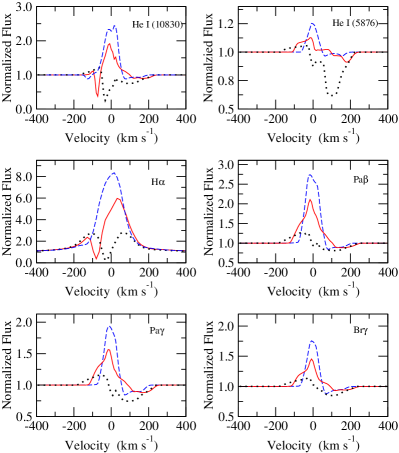
Figure 7: An example model calculation with a combination of axisymmetric magnetosphere and disc wind. The normalized model profile are shown as a function of velocity. The model parameters adopted here are: $T_{\mathrm{max}}=$7,500 K, $T_{\mathrm{dw}}=$9,000 K, $L_{\mathrm{X}}=2\times 10^{29}\,\mathrm{ergs^{-1}}$, and $\dot{M}_{\mathrm{a}}=10^{-7}\,\mathrm{M_{\sun}\,yr^{-1}}$, $\dot{M}_{\mathrm{dw}}=10^{-8}\,\mathrm{M_{\sun}\,yr^{-1}}$ (see text for other parameters). The profiles are computed at inclination angles $i=20^{\circ}$ (dashed), $50^{\circ}$ (solid) and $80^{\circ}$ (dotted). N.B. the lower limits of the vertical axis for He i (10830) and H$\alpha$ are set to 0, but those for He i (5876), Pa$\beta$, Pa$\gamma$ and Br$\gamma$ are set to 0.5.

As mentioned earlier, the sensitivity of He i $\lambda 10830$ to the innermost winds of CTTSs and its usefulness for proving the physical conditions of the winds have been well demonstrated in the past (e.g. Edwards et al. 2006; Kwan et al. 2007; Edwards 2009; Kwan & Fischer 2011). To test whether the magnetosphere–disc wind hybrid model can account for the types of He i $\lambda 10830$ profiles seen in the observations, we have run a small set of profile models for a various combinations of $\dot{M}_{\mathrm{dw}}$, $T_{\mathrm{dw}}$ and $i$. The rest of the parameters are kept same as in our canonical model shown in Fig. 7. We then examined if there is a resemblance between any of our model profiles to a set of He i $\lambda 10830$ line observations in Edwards et al. (2006). In the following, we present an example case in which the model profile morphology resembles that of an observation.

Fig. 8 shows a simple comparison of a He i $\lambda 10830$ line profile from our magnetosphere–disc wind hybrid model with the observed He i $\lambda 10830$ profile of UY Aur (CTTS; M0) obtained by Edwards et al. 2006. The model profile in the figure is computed with the following parameters: $T_{\mathrm{dw}}=$ 9,000 K, $\dot{M}_{\mathrm{dw}}=2.5\times 10^{-9}\,\mathrm{M_{\sun}\,yr^{-1}}$ and $i=48^{\circ}$. The mass-accretion rate for UY Aur adopted here ($\log\dot{M}_{\mathrm{a}}=-7.0$) is similar to the observationally estimated value of $\log\dot{M}_{\mathrm{a}}=-7.2$ (Edwards et al. 2006), but the adopted wind mass-loss rate is slightly smaller than the observed value of $\log\dot{M}_{\mathrm{w}}=-8.2$ (Edwards et al. 2006). The model reproduces the basic features of the observed He i $\lambda 10830$ line profile remarkably well. We find good matches of the model and the observation in: (1) the location and the narrowness of the blueshifted absorption line (caused by the disc wind), (2) the line strength, and (3) the depth and the width of the redshifted absorption (caused by the magnetospheric accretion). This clearly demonstrates the plausibility of our model (magnetosphere + disc wind) in explaining the type of line profile exhibited by UY Aur. Our model agrees with the earlier finding by Kwan et al. (2007) and Edwards (2009) who suggest that the relatively narrow blueshifted absorption seen in the observed He i $\lambda 10830$ line of UY Aur is likely caused by a disc wind.

In addition to He i $\lambda 10830$, we have also computed Pa$\gamma$ profile for UY Aur since the observation presented by Edwards et al. (2006) also includes Pa$\gamma$ (which is obtained simultaneously with He i $\lambda 10830$). The result is shown also in Fig. 8. Both model and the observation shows no sign of blueshifted wind absorption. A small amount of redshifted absorption is seen in both model and the observation. The overall agreement between the model and observed Pa$\gamma$ profiles is very good. An important difference between the model and observation is in the strength of the blue wing emission. The observation shows a very notable amount of emission in the wing ($V<-100\,\mathrm{km~{}s^{-1}}$). However, the model do not show this emission. This may suggest that the emission from the wind in UY Aur is much stronger than that of our model. To match the extended blue wing, we may need to adjust the wind temperature to a higher value. A further discussion on the blue wing emission will be given in Section 5.1.

Again, our main objective here is to test whether the magnetosphere–disc wind hybrid model can roughly account for the types of He i $\lambda 10830$ profiles seen in the observations, but is not to derive a set of physical parameters that is required to reproduce the observed line profile as this requires more careful analysis. In other words, the model profile shown here is not a strict fit to the observation. However, given the similarity of our model profiles with those of UY Aur, we should be able to derive the physical parameters of the accretion flow and wind around the object by performing the fine grid parameter search and performing the $\chi^{2}$ fitting to not only He i $\lambda 10830$ line but also to other hydrogen and helium lines, simultaneously. This is beyond the scope of this paper, but shall be left for a future investigation.

Figure 8: Example model calculations with a combination of axisymmetric magnetosphere and disc wind. The normalized model profiles (right panels) are compared with the observed line profiles (left panels) of UY Aur obtained by Edwards et al. (2006). The upper and lower panels show He i $\lambda$10830 and Pa$\gamma$ profiles, respectively. The observed profiles are obtained simultaneously (see Edwards et al. 2006 for detail). The inclination angle used for computing the model profiles is $i=48^{\circ}$. The model parameters adopted here are: $T_{\mathrm{max}}=$7,500 K, $T_{\mathrm{dw}}=$9,000 K, $L_{\mathrm{X}}=2\times 10^{29}\,\mathrm{ergs^{-1}}$, $\dot{M}_{\mathrm{a}}=10^{-7}\,\mathrm{M_{\sun}\,yr^{-1}}$, and $\dot{M}_{\mathrm{dw}}=2.5\times 10^{-9}\,\mathrm{M_{\sun}\,yr^{-1}}$. N.B. the model line profiles shown here are not strict fits to the observations, but are simple comparisons of the profile morphology.

4.3 Stellar wind model

4.3.1 Configuration

As shown in the observations of He i $\lambda 10830$ by Edwards et al. (2006), about 40 per cent of the CTTSs in their sample exhibit P-Cygni profiles. The observations indicate a possible presence of rapidly expanding stellar winds, in some of CTTSs. The stellar wind threaded by the open magnetic field in the polar region is a possible mechanism for angular momentum loss (e.g. Hartmann & MacGregor 1982; Mestel 1984; Hartmann & Stauffer 1989; Tout & Pringle 1992; Paatz & Camenzind 1996; Matt & Pudritz 2005; Matt & Pudritz 2008a; Matt & Pudritz 2008b; Matt et al. 2010). Recent work by Cranmer (2008) and Cranmer (2009) have shown a possible mechanism of heating and acceleration of the stellar wind, in the context of CTTSs, driven by accretion.

We replace the disc wind, described in Section 4.2.1, with the stellar wind, which arises only in the polar directions as shown in Fig. 9. Our stellar wind model consists of narrow cones with the half-opening angle $\theta_{\mathrm{sw}}$ in the polar directions ($\pm z$ direction as shown in the figure). The wind is assumed to be propagating only in the radial direction, and its velocity is described by the classical beta-velocity law (cf. Castor & Lamers 1979) i.e.

$$v_{r}\left(r\right)=v_{0}+\left(v_{\infty}-v_{0}\right)\left(1-\frac{R_{0}}{r}\right)^{\beta}\,,$$ (31)

where $v_{\infty}$ and $v_{0}$ are the terminal velocity and the velocity of the wind at the base ($r=R_{0}$). Assuming the mass-loss rate by the wind is $\dot{M}_{\mathrm{sw}}$ and using the mass-flux conservation in the flows in cones, the density $\rho_{\mathrm{sw}}$ of the wind can be written as:

$$\rho_{\mathrm{sw}}\left(r\right)=\frac{\dot{M}_{\mathrm{sw}}}{4\pi r^{2}v_{r}\left(r\right)\left(1-\cos\theta_{\mathrm{sw}}\right)}\,,$$ (32)

where $\theta_{\mathrm{sw}}>0$, and $\rho_{\mathrm{sw}}$ becomes that of a spherical wind when $\theta_{\mathrm{sw}}=90^{\circ}$. The temperature of the stellar wind ($T_{\mathrm{sw}}$) here is also assumed isothermal, as in the case for the disc wind model (Section 4.2.1).

When the wind is launched from the stellar surface (i.e. $R_{0}=R_{*}$), the half-opening angle $\theta_{\mathrm{sw}}$ is restricted to be less than $\sim 35^{\circ}$ to avoid an overlapping of the wind with the accretion funnels (cf. Fig. 9). On the other hand, if we assume that the wind is launched at a slightly larger, e.g. at the outer radius of the magnetosphere $R_{0}=R_{\mathrm{mo}}$, the opening angle of the wind is not restricted by the geometry of the accretion funnels. In the models presented in this paper, we adopt $R_{0}=R_{\mathrm{mo}}(=3.0\,R_{*})$ and $\theta_{\mathrm{sw}}=50^{\circ}$.

4.3.2 Example profiles

Fig. 10 shows the example helium and hydrogen profiles computed for the standard axisymmetric magnetospheric accretion funnels ($R_{\mathrm{mi}}=2.2\,R_{*}$, $R_{\mathrm{mo}}=3.0\,R_{*}$, $\dot{M}_{\mathrm{a}}=10^{-7}\,\mathrm{M_{\sun}\,yr^{-1}}$ and $T_{\mathrm{max}}=7,500\,\mathrm{K}$) and the stellar wind with the following parameters: $T_{\mathrm{sw}}=8,000\,\mathrm{K}$, $\dot{M}_{\mathrm{sw}}=10^{-8}\,\mathrm{M_{\sun}\,yr^{-1}}$, $\theta_{\mathrm{sw}}=50^{\circ}$, $v_{0}=10\,\mathrm{km~{}s^{-1}}$, $v_{\infty}=400\,\mathrm{km~{}s^{-1}}$, $R_{0}=3.0\,R_{*}$, and $\beta=0.5$ (cf. Section 4.3.1 and Fig. 9). The parameters for the central star are as described in Section 4.1.1. The effective temperature of the hotspot, as described in Section 4.1.2, is approximately 6,400 K. The X-ray luminosity of the chromosphere (cf. Section 4.1.3) is assumed to be $L_{\mathrm{X}}=2\times 10^{29}\,\mathrm{erg\,s^{-1}}$. The profiles shown here are computed for the system with the inclination angle of $i=53^{\circ}$. Note that the wind half opening angle $\theta_{\mathrm{sw}}$ here is much wider ($\sim 50^{\circ}$) than the one shown in Fig. 9 since the base of the stellar wind in this particular model is set to be at the outer radius of the magnetosphere ($R_{\mathrm{0}}=R_{\mathrm{mo}}$) instead of the stellar surface ($R_{\mathrm{0}}=R_{\mathrm{*}}$). The stellar and disk occultations are taken into account in our profile calculations.

As in the disc wind cases (Section 4.2.2), we have adopted a relatively low stellar wind temperature (8,000 $\mathrm{K}$) here to avoid unrealistically strong emission in the hydrogen lines, produced at the base of the wind. Again, for the same reason, the temperature of the magnetosphere cannot be much higher than $T_{\mathrm{max}}=7,500\,\mathrm{K}$ (for the system with $\dot{M}_{\mathrm{a}}=10^{-7}\,\mathrm{M_{\sun}\,yr^{-1}}$). As done for the disc wind case, we have added the X-ray flux (as described in Section  4.1.3) in the stellar radiation as an additional source of photoionization. This helps to populate the excited states of He i and to produce a reasonable line strength in He i $\lambda$10830. The resulting profiles are shown in Fig. 10.

The He i $\lambda$10830 profiles (Fig. 10), computed at the low and intermediate inclination angles ($i=20^{\circ}$ and $50^{\circ}$), show the absorption features in both red and blue wings. However, unlike the disc wind case, the blueshifted absorption is much wider and it extends almost to the terminal velocity of the wind, $v_{\infty}=400\,\mathrm{km~{}s^{-1}}$. This is the classical P-Cygni profile which is caused by the expanding stellar wind. As mentioned earlier, about 40 per cent of the CTTSs in the observations of Edwards et al. (2006) show the P-Cygni profiles in He i $\lambda 10830$. The model profile of the He i $\lambda 10830$ also shows the absorption in the red wing, which is caused by the magnetospheric accretion funnel (inflow). Again, the redshifted absorption component is also commonly (47 per cent) found in the observed He i $\lambda 10830$ profiles of Edwards et al. (2006).

The model line profiles of He i $\lambda$5876 (Fig. 10) are very similar to those computed with the disc wind (Fig. 7). Again, there is no clear sign of a blueshifted wind absorption in the models. The similarity of the profiles here with those of the disk wind model (Fig. 7) and the fact that the physical conditions (the density, temperature and velocity) of the magnetospheres used here are exactly the same as in the models with the disc wind (Fig. 7) suggests that, at least with this particular set of model parameters, the emission in He i $\lambda$5876 mainly occurs in the magnetosphere. As in the disc wind case, He i $\lambda$5876 profiles are much weaker than He i $\lambda 10830$ profiles. The line ratio of He i $\lambda$5876 and He i $\lambda 10830$ (using their peak fluxes) is about $\sim 0.07$ for the line profiles computed at the intermediate inclination angle $i=50^{\circ}$. As mentioned earlier, the redshifted absorption in He i $\lambda$5876 is rather rare (about 10 per cent) in the observation of Beristain et al. (2001) (see also Alencar & Basri 2000).

The H$\alpha$ profile here also shows a broad wing in red, extending up to $+400\,\mathrm{\mathrm{km~{}s^{-1}}}$. The blue wing is strongly affected by the presence of the wind absorption component for the models computed at $i=50^{\circ}$ and $80^{\circ}$. Similar to He i $\lambda$10830, the blueshifted absorption in the H$\alpha$ profile is wide and it extends almost to $v_{\infty}=400\,\mathrm{km~{}s^{-1}}$. This profile can be also classified as a P-Cygni profile. Unlike He i $\lambda$10830, the redshifted absorption does not go below the continuum level in this H$\alpha$ profile. Based on the morphology of the profile, it is classified as ‘Type IV-B’ according the classification scheme of Reipurth et al. (1996). This type of line profile is relatively rare ($\sim$7 per cent) in the observed H$\alpha$ profiles of Reipurth et al. (1996).

As we found in the disc wind case (Section 4.2), the wind signature (the blueshifted absorption component) is absent in the model profiles of Pa$\beta$ and Br$\gamma$. Only the redshifted absorption component cased by the accreting gas in the magnetosphere is present (the IPC profiles). This is consistent with the near infrared spectroscopic observations of 50 T Tauri stars by Folha & Emerson (2001). The model profiles of Pa$\beta$ and Br$\gamma$ shown here are very similar to those of the disc wind model (in Fig. 7) because these lines are not affected by the presence of the wind, and the inclinations ($i$) used in both models are same. The wind signature is also absent in Pa$\gamma$ profiles shown in Fig. 10. As mentioned earlier, this is consistent with the observation of Edwards et al. (2006). Again, the morphology of the Pa$\gamma$ model profiles shown here overall agrees with the ranges of the profile shapes found in the observation of Edwards et al. (2006).

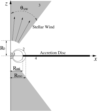
Figure 9: Same as in Fig. 6, but for the (bipolar) stellar wind and magnetospheric accretion hybrid model. The system consists of four components: (1) the continuum source located at the origin of the cartesian coordinates $\left(x,y,z\right)$ – the $y$-axis is into the paper, (2) the magnetospheric accretion flow, (3) the stellar wind, and (4) the optically thick but geometrically thin accretion disc. The wind is launched from a sphere with radius $R_{0}$, but is restricted within the cones with the half opening angle $\theta_{\mathrm{sw}}$. We adopt $R_{0}=R_{\mathrm{mo}}(=3.0~{}R_{*})$ and $\theta_{\mathrm{sw}}=50^{\circ}$ for the models presented in this paper. The density distribution is symmetric around the $z$-axis. The figure is not to scale.

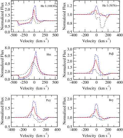
Figure 10: An example model calculation with a combination of axisymmetric magnetosphere and a stellar wind. The normalized model profile are shown as a function of velocity. The model parameters adopted here are: $T_{\mathrm{max}}=$ 7,500 K, $T_{\mathrm{sw}}=$ 8,000 K, $\dot{M}_{\mathrm{a}}=10^{-7}\,\mathrm{M_{\sun}\,yr^{-1}}$, $\dot{M}_{\mathrm{sw}}=10^{-8}\,\mathrm{M_{\sun}\,yr^{-1}}$, and $L_{\mathrm{X}}=2\times 10^{29}\,\mathrm{erg\,s^{-1}}$. The profiles are computed at inclination angles $i=20^{\circ}$ (dashed), $50^{\circ}$ (solid) and $80^{\circ}$ (dotted). N.B. the lower limits of the vertical axis for He i (10830) and H$\alpha$ are set to 0, but those for He i (5876), Pa$\beta$, Pa$\gamma$ and Br$\gamma$ are set to 0.5.

As in the disc wind case, we now test whether the magnetosphere–stellar wind hybrid model can roughly account for the types of He i $\lambda 10830$ profiles seen in the observations. We have run a small set of profile models for a various combinations of $\dot{M}_{\mathrm{sw}}$, $T_{\mathrm{sw}}$, $i$, and the turbulence velocity in the magnetosphere and the wind. Note that no turbulence velocity is included in the previous models. The rest of the parameters are kept same as in our canonical model shown in Fig. 10. We then examined if there is a resemblance between any of our model profiles to a set of He i $\lambda 10830$ line observations in Edwards et al. (2006).

Fig. 11 shows a simple comparison of a He i $\lambda 10830$ line profile from our magnetosphere–stellar wind hybrid model with the observed He i $\lambda 10830$ profile of AS 353 A (CTTS; K5) from Edwards et al. (2006). The model profile in the figure is computed with the following parameters: $T_{\mathrm{sw}}=$ 8,000 K, $\dot{M}_{\mathrm{\mathrm{sw}}}=2.5\times 10^{-8}\,\mathrm{M_{\sun}\,yr^{-1}}$, $L_{\mathrm{X}}=1\times 10^{29}\,\mathrm{erg\,s^{-1}}$, $i=10^{\circ}$, and the turbulence velocity of 80 $\mathrm{km~{}s^{-1}}$ in both the magnetosphere and the wind. The rest of the parameters are same as those used in Fig. 10. Note that the mass-accretion rate for AS 353 A adopted here ($\log\dot{M}_{\mathrm{a}}=-7.0$) is much smaller than the observationally estimated value of $\log\dot{M}_{\mathrm{a}}=-5.4$ (Edwards et al. 2006), but the adopted wind mass-loss rate is very smaller to the observed value of $\log\dot{M}_{\mathrm{w}}=-7.6$ (Edwards et al. 2006).

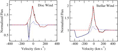
Figure 12: Comparisons of model He i $\lambda 10830$ line profiles computed with different flow elements in the disc wind + magnetosphere configuration (left panel) and in the stellar wind + magnetosphere configuration (right panel). The profiles are computed with (1) the magnetosphere only (dashed), (2) the disc/stellar wind only (dotted), and (3) the combination of the magnetosphere and disc/stellar wind (solid). The physical parameters used here are the same as those in Figs. 7 and 10 for the models with the disc wind and that with the stellar wind, respectively. The inclination angle $i=50^{\circ}$ is used for all the models.

By following Kwan et al. (2007), to match the location of the emission peak in red ($\sim 200\,\mathrm{km~{}s^{-1}}$), a relatively high turbulence velocity (80 $\mathrm{km~{}s^{-1}}$ in both the magnetosphere and the wind) is added to the model. Note that Kwan et al. (2007) applied a high turbulence velocity in the wind only, but not in the magnetosphere — their model does not include a magnetosphere at all. As we demonstrate later in Section 5.1 (Fig. 12), the line ‘emission’ mainly arises from the magnetosphere in the models presented in this paper; therefore, it is not possible to match the peak of the observed profile without invoking a significant (80 $\mathrm{km~{}s^{-1}}$) turbulence velocity also in the magnetospheric accretion funnels. This essentially arbitrary line-broadening (over-and-above thermal and pressure broadening) may have a physical basis in the magnetically-channelled nature of the inflows and outflows, and further radiative transfer models will be necessary to investigate whether it would be possible to determine whether the different turbulent broadening may apply in both the wind and the accretion streams. If one could find a solution in which the wind emission dominates, the high turbulence velocity in the magnetosphere assumed here might not be necessary.

The figure shows that the magnetosphere–stellar wind hybrid model reproduces the basic features of the observed He i $\lambda 10830$ line profile relatively well. The model profile shows a clear P-Cygni profile, and the overall agreement of the model and the observational line profile morphology is very well. Again, this demonstrates the plausibility of our model (magnetosphere + stellar wind) in explaining the type of line profile exhibited by AS 353 A. Our model agrees with the earlier finding by Kwan et al. (2007) and Edwards (2009) who suggest that the relatively wide blueshifted absorption (the P-Cygni profile) seen in the observed He i $\lambda 10830$ line of AS 353 A is likely caused by a stellar wind.

We have also computed Pa$\gamma$ profile for AS 353 A, and compared it with the observed profile from Edwards et al. (2006). The data is acquired simultaneously with the He i $\lambda 10830$ line. The profiles are also shown in Fig. 11. No clear sign of wind absorption is seen in both model and observed Pa$\gamma$ profiles. Note that the line width of the model Pa$\gamma$ profile in Fig. 11 is much larger than that of the Pa$\gamma$ profile in Fig. 10 (for $i=20^{\circ}$ case) because of the high turbulence velocity (80 $\mathrm{km~{}s^{-1}}$) in the magnetosphere used in the model for AS 353 A. The model shows a weak redshifted absorption, but the observation does not. The line strength of the model is noticeably weaker than the observed profile. Another important difference between the model and observation is in the amount of the emission in the wings of the profiles. The observation shows significant emissions in the wing extending up to $V\sim\pm 400\,\mathrm{km~{}s^{-1}}$. On the other hand, our model do not show strong wing emissions. This difference was also found in the comparison of Pa$\gamma$ profiles in UY Aur (Fig. 8). To produce the extended wing emission and a stronger line centre flux in our model, a higher wind temperature may be needed. A further discussion on the extended wing emissions will be given in Section 5.1.

Once again, our main objective here is to demonstrate whether the magnetosphere–stellar wind hybrid model can roughly account for the types of He i $\lambda 10830$ profiles seen in the observations, but is not to derive a set of physical parameters that is required to reproduce the observed line profile as this requires more careful analysis. For example, the mass-accretion rate used here is much smaller than the observed value and it should not be considered as a derived model parameter. However, the resemblance of the model profiles to those of AS 353 A suggests a possibility for deriving the physical parameters of the accretion flow and wind around the object by performing the fine grid parameter search and performing the $\chi^{2}$ fitting to a set of (preferably) simultaneously observed multiple hydrogen and helium lines (including He i $\lambda 10830$).

Figure 11: Example model calculations with a combination of axisymmetric magnetosphere and a stellar wind. The normalized model profiles (right panels) are compared with the observed line profiles (left panels) of AS 353 A obtained by Edwards et al. (2006). The upper and lower panels show He i $\lambda$10830 and Pa$\gamma$ profiles, respectively. The observed profiles are obtained simultaneously (see Edwards et al. 2006 for detail). The inclination angle used for computing the model profiles is $i=10^{\circ}$. The model parameters adopted here are: $T_{\mathrm{max}}=$7,500 K, $T_{\mathrm{sw}}=$8,000 K, $L_{\mathrm{X}}=1\times 10^{29}\,\mathrm{ergs^{-1}}$, $\dot{M}_{\mathrm{a}}=10^{-7}\,\mathrm{M_{\sun}\,yr^{-1}}$, and $\dot{M}_{\mathrm{sw}}=2\times 10^{-9}\,\mathrm{M_{\sun}\,yr^{-1}}$. N.B. the model line profiles shown here are not strict fits to the observations, but are simple comparisons of the profile morphology.

5 Discussions

5.1 Some unresolved issues

While the blue and redshifted absorption components in the model line profiles (e.g. in Figs. 7 and 10) could provide us the physical conditions and locations of line ‘absorption’, the locations of line ‘emission’ are not so straightforwardly understood from the model profiles. To demonstrate which gas flow component (magnetosphere or wind) contributes to the emission part of the profiles, we compare the He i $\lambda 10830$ line profiles computed using (1) the magnetosphere only, (2) the disc/stellar wind only, and (3) the combination of the magnetosphere and disc/stellar wind. The results are placed in Fig. 12. The physical parameters used here are the same as those in Figs. 7 and 10 for the models with the disc wind and that with the stellar wind, respectively. As one can see from the figure, with these particular sets of model parameters, mainly the magnetospheres contribute to the emission. The wind emission is relatively low, and the winds mainly contribute to blueshifted absorptions. Although not shown here, the magnetosphere is also a main emission contributor in other lines shown in Figs. 7 and 10. Since we have not yet surveyed a large parameter space for the wind and magnetosphere in our models, we cannot generalise the statement above. The relative importance of the wind and magnetospheric emission and the determination of the emission location require further investigation which we defer to a future study.

There are at least two important differences between the model profiles, computed with the magnetosphere as a main line emitter, and observed profiles. Firstly, the line widths of Pa$\beta$ and Br$\gamma$ in our models (e.g. Figs. 7 and 10) are much narrower than those from the observation by Folha & Emerson (2001). The full width half-maxima (FWHM) of Pa$\beta$ and Br$\gamma$ are about 200 $\mathrm{km~{}s^{-1}}$ in Folha & Emerson (2001), but those in our model are $\sim 100$ or less. Since the maximum infall velocity in our model is essentially limited to the escape velocity from the star ($\sim 300\,\mathrm{km~{}s^{-1}}$ with $R_{*}=2\,R_{\odot}$ and $M_{*}=0.5\,M_{\odot}$), it is hard to achieve the FWHM values found in the observation without an additional form of line broadening (e.g. turbulence broadening). Kurosawa et al. (2006) also discuss a similar problem. The emission from a stronger wind may also help to make the lines broader, but the stronger wind would also cause a blueshifted absorption.

Secondly, the extent of the blue wing emission in the model profiles are much smaller than those found in observations. In the comparison of the model profiles with the observation of UY Aur (Fig. 8), we found the blue wings of the observed He i $\lambda 10830$ and Pa$\gamma$ extend up to $\sim 300\,\mathrm{km~{}s^{-1}}$ while our models show the blue wings only up to $\sim 130\,\mathrm{km~{}s^{-1}}$. Similarly for AS 353 A (see Fig. 11), the blue wing of the observed Pa$\gamma$ profile extends up to $\sim 400\,\mathrm{km~{}s^{-1}}$ while that of the model extends only up to $~{}200\,\mathrm{km~{}s^{-1}}$, even with a large turbulence velocity ($80\,\mathrm{km~{}s^{-1}}$) included. As mentioned earlier, in the models considered here, the line emission mainly arises in the magnetosphere. Hence, with this set up, the models have difficulties in producing the blue wing emission extending to such high velocity. This discrepancy may suggest that the emission from a fast wind (a disc or stellar wind) may be necessary to reproduce the extended blue wing emission seen in the emission. Whether one can reproduce the strong blue wing emission by a wind without causing a strong blueshifted absorption and a (too) strong central emission component is still unknown. This issue will be investigated further in a future study.

As we have briefly mentioned in Section 4.3.2, H$\alpha$ lines computed with the stellar wind + magnetospheric accretion (see Fig. 10) exhibit strong P-Cygni like blueshifted absorptions; however, this type of profile (Type IV-B in the classification by Reipurth et al. 1996) is rare in the observations. In our model configuration (with a stellar wind), it is difficult not to produce a P-Cygni like absorption when we require a P-Cygni like absorption in He i $\lambda 10830$. In other words, whenever a P-Cygni like absorption is present in He i $\lambda 10830$, it also appears in H$\alpha$. One possible way to avoid this problem is to use a lower wind temperature which reduces the ionization level of hydrogen in the wind, but not that of helium since the helium ionization level is mainly controlled by the X-ray flux. Another possibility is to increase the temperature of the magnetosphere which would increase the emission in the wings of H$\alpha$ and would suppress the strong blue absorption features. This point shall also be investigated further in a future study.

5.2 X-ray optical depths

When computing the statistical equilibrium of the atomic population levels, we have neglected the attenuation of X-ray emission by implicitly assuming the radiation is optically thin. Here we examine whether this assumption is reasonable, by computing the X-ray optical depth (continuum) using the ionization structure found in the disc wind plus magnetospheric accretion model shown in Fig. 7 (Section 4.2.2) and also the stellar wind plus magnetospheric accretion model shown in Fig. 10 (Section 4.3.2). Note that the optical depths computed from these models are not self-consistent since the inclusion of the X-ray attenuation should, in principle, alter the ionization structures itself, especially for He i. Hence, the following optical depth values are merely rough estimates.

For the photon energy $\epsilon=0.1$ keV and along a line of sight to an observer at $i=50^{\circ}$, the optical depth across the magnetospheric accretion stream is $\tau_{\mathrm{X}}\approx 10^{3}$, and that across the wind is $\tau_{\mathrm{X}}\approx 20$ and $\approx 40$ for the disc wind and stellar winds, respectively. On the other hand, for $\epsilon=1.0$ keV, $\tau_{\mathrm{X}}\approx 1$ for the magnetosphere, and $\tau_{\mathrm{X}}\approx 0.01$ and $\approx 0.02$ for the disc and stellar winds respectively. The optical depths are computed with the models with the mass-accretion $\dot{M}_{\mathrm{a}}=10^{-7}\,\mathrm{M_{\sun}\,yr^{-1}}$ and the wind mass-loss rate $\dot{M}_{\mathrm{w}}=10^{-8}\,\mathrm{M_{\sun}\,yr^{-1}}$, which are about 10 times higher than those of a typical CTTS. If more typical values are used (i.e. $\dot{M}_{\mathrm{a}}=10^{-8}\,\mathrm{M_{\sun}\,yr^{-1}}$ and $\dot{M}_{\mathrm{w}}=10^{-9}\,\mathrm{M_{\sun}\,yr^{-1}}$), the optical depths would be about 10 times lower than the values shown above. In our model, the main source of the continuum opacity around the photon energy 0.1 keV is the bound-free opacity of He i.

The high optical depths at 0.1 keV indicates that the most of the X-ray at this energy could not penetrate the high density magnetospheric accretion streams. On the other hand, the optical depth across the magnetosphere at 1.0 keV is marginal ($\tau_{\mathrm{X}}\sim 1.0$), and may penetrate the accretion streams, after its intensity being reduced by a factor of $e^{\tau_{\mathrm{X}}}\sim 2.7$. This suggests that our He i line strength may be overestimated for a given amount of X-ray luminosity. In reality, the magnetospheric accretion may not be completely axisymmetric, and the accretion would occur only in two or more funnel streams as shown by 3D MHD simulations (e.g. Romanova et al. 2003). This indicates a presence of large gaps between the funnel flows; hence, a significant fraction of the X-ray produced near the stellar surface could still reach to the stellar or disc wind by escaping though the gaps, and ionize He i in the wind. We plan to implement a proper treatment of X-ray attenuation effect in a future model.

6 Summary and conclusions

The radiative transfer code torus (Harries 2000; Kurosawa et al. 2004; Symington et al. 2005: Kurosawa et al. 2006; Kurosawa et al. 2008) is extended to include helium atoms (19 levels for He i, 10 levels for He ii and the continuum level for He iii). Only hydrogen atoms (up to 20 levels) are included in the previous versions of the code. The addition of helium atoms in our code is motivated by the recent observations of Edwards et al. (2003), Dupree et al. (2005) and Edwards et al. (2006) who demonstrated a robustness of optically thick He i $\lambda 10830$ as a diagnostic tool for probing the innermost wind of CTTSs.

We have tested our new implementation of the statistical equilibrium routine which simultaneously solves H and He level populations (Section 3.1) by comparing the model with the non-LTE line-blanketed atmosphere code cmfgen (Hillier & Miller 1998) in which the level populations are solved in a spherical geometry (1D). For the case of spherically expanding hot stellar wind (AV 83), we have found a good agreement between torus and cmfgen in computing the number fractions of He ions (Fig. 2), opacities (Fig. 3), and observed line profiles (Fig. 4). The code has been also tested in a 2D (axisymmetric) geometry (Section 3.2). The emission line profile models of Muzerolle et al. (2001), who used the axisymmetric magnetospheric accretion model of Hartmann et al. (1994), have been well reproduced with our model (Fig. 5).

We have also demonstrated the capabilities of our newly implemented code in the line formation problems of CTTSs (Section 4). We have considered two different combinations of the inflow and outflow geometries: (1) the magnetospheric accretion and the disc wind (Section 4.2), and (2) the magnetospheric accretion and the bipolar stellar wind (Section 4.3). In both cases, our models are able to produce line profiles similar to the observed ones (e.g. Edwards et al. 1994; Reipurth et al. 1996; Folha & Emerson 2001; Edwards et al. 2006), in the morphology and the line strengths (Figs. 7 and 10). In particular, the comparison of the model He i $\lambda 10830$ profiles with with the observations of Edwards et al. (2006) (Figs. 8 and 11) suggests that the relatively deep and wide blueshifted absorption component found in some CTTSs is most likely caused by the bipolar stellar wind while the narrower blueshifted absorption is caused by the disc wind (cf. Kurosawa et al. 2006; Kwan et al. 2007).

During our initial investigation of the simultaneous modelling of H and He emission lines, we found (in both the disc wind and stellar wind cases) the temperature of the wind must be relatively low e.g. $T\sim$10,000 K (for $\dot{M}_{\mathrm{a}}=10^{-7}\,\mathrm{M_{\sun}\,yr^{-1}}$ and it could be slightly higher for a lower mass-accretion rate), and it is likely below 20,000 K. The line strengths of hydrogen lines (e.g. H$\alpha$) will be unrealistically strong if the temperature is much higher. On the other hand, at this relatively low wind temperature ($T\sim$10,000 K), the collisional rates of He i are too low, and the normal continuum sources (the photosphere with $T_{\mathrm{eff}}\sim$4,000 K and the hot spot with $T_{\mathrm{hs}}\sim$6,400 K or even with $T_{\mathrm{hs}}\sim$8,000 K) do not provide enough radiation to ionize/excite He i significantly. To populate the excited states of He i and hence to produce He i $\lambda 10830$ with a realistic line strength (c.f. Figs. 8 and 11), one requires a high energy radiation source such as X-ray radiation. Interestingly, a recent work by Kwan & Fischer (2011) has shown that UV photoionization is also a probable excitation mechanism for generating He i $\lambda 10830$ opacities. From the observations of TW Hya and RU Lup, Johns-Krull & Herczeg (2007) also reached a similar conclusion. Both our model and the work by Kwan & Fischer (2011) suggest a need for the extra photoionizing radiation sources. The relative importance of the UV and X-ray luminosity is not known at this moment.

The following is the list of a several key questions which are yet to be answered: Do the stellar wind and disc wind coexist? In which physical condition, one dominates the other? What are the possible ranges of temperature and density in the winds? Must the winds of CTTS be clumpy (inhomogeneous), as suggested by Kwan & Fischer (2011)? What is the relative importance of the UV and X-ray? Where exactly is the location of X-ray emission? We intent to investigate and provide answers to some or most of the questions mentioned above in our subsequent papers in the future.

Finally, we also plan to apply our radiative transfer model to the results of 2D and 3D MHD simulations of the (innermost) conical wind and magnetospheric accretion of CTTSs by Romanova et al. (2009). A direct comparison of the MHD simulations with observations is difficult, but it can be mediated by modelling emission line profiles which could constrain some basic physical parameters of the flow such as the geometry, temperature and mass accretion and outflow rates. In turn, these parameters can provide constraints on the amount of angular momentum transfer to and out of the stars. By using the different time slices of the MHD simulations, we will be also able to address the issues of the time-variability in the line and continuum by comparing the models with observations (e.g. Kurosawa et al. 2008).

References

- Acreman et al. (2010) Acreman D. M., Harries T. J., Rundle D. A., 2010, MNRAS, 403, 1143
- Alencar & Basri (2000) Alencar S. H. P., Basri G., 2000, AJ, 119, 1881
- Alencar et al. (2005) Alencar S. H. P., Basri G., Hartmann L., Calvet N., 2005, A&A, 440, 595
- Alexander (2008) Alexander R., 2008, New Astron. Rev., 52, 60
- Argiroffi et al. (2007) Argiroffi C., Maggio A., Peres G., 2007, A&A, 465, L5
- Bergin (2009) Bergin E. A., 2009, preprint (astro-ph/0908.3708)
- Beristain et al. (2001) Beristain G., Edwards S., & Kwan J., 2001, ApJ, 551, 1037
- Blandford & Payne (1982) Blandford R. D., Payne D. G., 1982, MNRAS, 199, 883
- Calvet & Gullbring (1998) Calvet N., Gullbring E., 1998, ApJ, 509, 802
- Castor (1970) Castor J. I., 1970, MNRAS, 149, 111
- Castor et al. (1975) Castor J. I., Abbott D. C., Klein R. I., 1975, ApJ, 195, 157
- Castor & Lamers (1979) Castor J. I., Lamers H. J. G. L. M., 1979, ApJS, 39, 481
- Cranmer (2008) Cranmer S. R., 2008, ApJ, 689, 316
- Cranmer (2009) —, 2009, ApJ, 706, 824
- Crowther et al. (1999) Crowther P. A., Pasquali A., De Marco O., Schmutz W., Hillier D. J., de Koter A., 1999, A&A, 350, 1007
- De Marco et al. (2000) De Marco O., Schmutz W., Crowther P. A., Hillier D. J., Dessart L., de Koter A., Schweickhardt J., 2000, A&A, 358, 187
- Dessart et al. (2000) Dessart L., Crowther P. A., Hillier D. J., Willis A. J., Morris P. W., van der Hucht K. A., 2000, MNRAS, 315, 407
- Dupree et al. (2005) Dupree A. K., Brickhouse N. S., Smith G. H., Strader J., 2005, ApJ, 625, L131
- Edwards (2007) Edwards S., 2007, in IAU Symp., Vol. 243, Star-Disk Interaction in Young Stars, Bouvier J., Appenzeller I., eds., p. 171
- Edwards (2009) Edwards S., 2009, in American Institute of Physics Conference Series, Vol. 1094, American Institute of Physics Conference Series, E. Stempels, ed., pp. 29–38
- Edwards et al. (2006) Edwards S., Fischer W., Hillenbrand L., Kwan J., 2006, ApJ, 646, 319
- Edwards et al. (2003) Edwards S., Fischer W., Kwan J., Hillenbrand L., Dupree A. K., 2003, ApJ, 599, L41
- Edwards et al. (1994) Edwards S., Hartigan P., Ghandour L., Andrulis C., 1994, AJ, 108, 1056
- Ercolano et al. (2009) Ercolano B., Clarke C. J., Drake J. J., 2009, ApJ, 699, 1639
- Ercolano et al. (2008) Ercolano B., Drake J. J., Raymond J. C., Clarke C. C., 2008, ApJ, 688, 398
- Feigelson & Montmerle (1999) Feigelson E. D., Montmerle T., 1999, ARA&A, 37, 363
- Ferreira et al. (2006) Ferreira J., Dougados C., Cabrit S., 2006, A&A, 453, 785
- Folha & Emerson (2001) Folha D. F. M., Emerson J. P., 2001, A&A, 365, 90
- Gagné et al. (2004) Gagné M., Skinner S. L., Daniel K. J., 2004, ApJ, 613, 393
- Ghosh et al. (1977) Ghosh P., Pethick C. J., Lamb F. K., 1977, ApJ, 217, 578
- Glassgold et al. (2004) Glassgold A. E., Najita J., Igea J., 2004, ApJ, 615, 972
- Güdel et al. (2010) Güdel M., Lahuis F., Briggs K. R., Carr J., Glassgold A. E., Henning T., Najita J. R., van Boekel R., van Dishoeck E. F., 2010, A&A, 519, 113
- Güdel et al. (2008) Güdel M., Skinner S. L., Audard M., Briggs K. R., Cabrit S., 2008, A&A, 478, 797
- Güdel & Telleschi (2007) Güdel M., Telleschi A., 2007, A&A, 474, L25
- Gullbring et al. (2000) Gullbring E., Calvet N., Muzerolle J., Hartmann L., 2000, ApJ, 544, 927
- Harries (1995) Harries T. J., 1995, PhD thesis, , University College, London, (1995)
- Harries (2000) —, 2000, MNRAS, 315, 722
- Harries et al. (2004) Harries T. J., Monnier J. D., Symington N. H., Kurosawa R., 2004, MNRAS, 350, 565
- Hartmann et al. (1982) Hartmann L., Avrett E., Edwards S., 1982, ApJ, 261, 279
- Hartmann et al. (1994) Hartmann L., Hewett R., Calvet N., 1994, ApJ, 426, 669
- Hartmann & MacGregor (1982) Hartmann L., MacGregor K. B., 1982, ApJ, 259, 180
- Hartmann & Stauffer (1989) Hartmann L., Stauffer J. R., 1989, AJ, 97, 873
- Herald et al. (2001) Herald J. E., Hillier D. J., Schulte-Ladbeck R. E., 2001, ApJ, 548, 932
- Herbst et al. (2007) Herbst W., Eislöffel J., Mundt R., Scholz A., 2007, in Protostars and Planets V, Reipurth B., Jewitt D., Keil K., eds., pp. 297–311
- Hillier et al. (2006) Hillier D. J. et al., 2006, ApJ, 642, 1098
- Hillier et al. (2003) Hillier D. J., Lanz T., Heap S. R., Hubeny I., Smith L. J., Evans C. J., Lennon D. J., Bouret J. C., 2003, ApJ, 588, 1039
- Hillier & Miller (1998) Hillier D. J., Miller D. L., 1998, ApJ, 496, 407
- Hillier & Miller (1999) —, 1999, ApJ, 519, 354
- Hirose et al. (1997) Hirose S., Uchida Y., Shibata K., Matsumoto R., 1997, PASJ, 49, 193
- Jardine et al. (2006) Jardine M., Cameron A. C., Donati J., Gregory S. G., Wood K., 2006, MNRAS, 367, 917
- Johns-Krull & Herczeg (2007) Johns-Krull C. M., Herczeg G. J., 2007, ApJ, 655, 345
- Kastner et al. (2002) Kastner J. H., Huenemoerder D. P., Schulz N. S., Canizares C. R., Weintraub D. A., 2002, ApJ, 567, 434
- Klein & Castor (1978) Klein R. I., Castor J. I., 1978, ApJ, 220, 902
- Knigge et al. (1995) Knigge C., Woods J. A., Drew E., 1995, MNRAS, 273, 225
- Königl & Pudritz (2000) Königl A., Pudritz R. E., 2000, Protostars and Planets IV, 759
- Königl et al. (2011) Königl A., Romanova M. M., Lovelace R. V. E., 2011, submitted to MNRAS
- Krasnopolsky et al. (2003) Krasnopolsky R., Li Z.-Y., Blandford R. D., 2003, ApJ, 595, 631
- Kurosawa et al. (2004) Kurosawa R., Harries T. J., Bate M. R., Symington N. H., 2004, MNRAS, 351, 1134
- Kurosawa et al. (2005) Kurosawa R., Harries T. J., Symington N. H., 2005, MNRAS, 358, 671
- Kurosawa et al. (2006) Kurosawa R., Harries T. J., Symington N. H., 2006, MNRAS, 370, 580
- Kurosawa & Hillier (2001) Kurosawa R., Hillier D. J., 2001, A&A, 379, 336
- Kurosawa et al. (2008) Kurosawa R., Romanova M. M., Harries T. J., 2008, MNRAS, 385, 1931
- Kurucz (1979) Kurucz R. L., 1979, ApJS, 40, 1
- Kwan et al. (2007) Kwan J., Edwards S., Fischer W., 2007, ApJ, 657, 897
- Kwan & Fischer (2011) Kwan J., Fischer W., 2011, MNRAS, 411, 2383
- Kwan & Tademaru (1988) Kwan J., Tademaru E., 1988, ApJ, 332, L41
- Lamzin (1998) Lamzin S. A., 1998, Astronomy Reports, 42, 322
- Lii et al. (2011) Lii P., Romanova M., Lovelace R., 2011, preprint (astro-ph/1104.4374)
- Lima et al. (2010) Lima G. H. R. A., Alencar S. H. P., Calvet N., Hartmann L., Muzerolle J., 2010, A&A, 522, A104
- Long & Knigge (2002) Long K. S., Knigge C., 2002, ApJ, 579, 725
- Luttermoser & Johnson (1992) Luttermoser D. G., Johnson H. R., 1992, ApJ, 388, 579
- Martins et al. (2005) Martins F., Schaerer D., Hillier D. J., 2005, A&A, 436, 1049
- Matt & Pudritz (2005) Matt S., Pudritz R. E., 2005, ApJ, 632, L135
- Matt & Pudritz (2007a) —, 2007a, in IAU Symp., Vol. 243, Star-Disk Interaction in Young Stars, Bouvier J., Appenzeller I., eds., p. 299
- Matt & Pudritz (2007b) —, 2007b, preprint (astro-ph/0701648)
- Matt & Pudritz (2008a) —, 2008a, ApJ, 678, 1109
- Matt & Pudritz (2008b) —, 2008b, ApJ, 681, 391
- Matt et al. (2010) Matt S. P., Pinzón G., de la Reza R., Greene T. P., 2010, ApJ, 714, 989
- Mestel (1984) Mestel L., 1984, in Lecture Notes in Physics, Berlin Springer Verlag, Vol. 193, Cool Stars, Stellar Systems, and the Sun, S. L. Baliunas & L. Hartmann, ed., p. 49
- Mihalas (1978) Mihalas D., 1978, Stellar atmospheres, 2nd edn. W. H. Freeman and Co., San Francisco
- Murphy et al. (2010) Murphy G. C., Ferreira J., Zanni C., 2010, A&A, 512, A82
- Muzerolle et al. (1998) Muzerolle J., Calvet N., Hartmann L., 1998, ApJ, 492, 743
- Muzerolle et al. (2001) —, 2001, ApJ, 550, 944
- Orlando et al. (2010) Orlando S., Sacco G. G., Argiroffi C., Reale F., Peres G., Maggio A., 2010, A&A, 510, A71
- Ouyed & Pudritz (1997) Ouyed R., Pudritz R. E., 1997, ApJ, 482, 712
- Owen et al. (2010) Owen J. E., Ercolano B., Clarke C. J., 2010, preprint (astro-ph/1010.0826)
- Paatz & Camenzind (1996) Paatz G., Camenzind M., 1996, A&A, 308, 77
- Preibisch et al. (2005) Preibisch T. et al., 2005, ApJS, 160, 401
- Pudritz et al. (2007) Pudritz R. E., Ouyed R., Fendt C., Brandenburg A., 2007, in Protostars and Planets V, Reipurth B., Jewitt D., Keil K., eds., University of Arizona Press, p. p. 277
- Reipurth et al. (1996) Reipurth B., Pedrosa A., Lago M. T. V. T., 1996, A&AS, 120, 229
- Romanova et al. (1997) Romanova M. M., Ustyugova G. V., Koldoba A. V., Chechetkin V. M., Lovelace R. V. E., 1997, ApJ, 482, 708
- Romanova et al. (2004) Romanova M. M., Ustyugova G. V., Koldoba A. V., Lovelace R. V. E., 2004, ApJ, 610, 920
- Romanova et al. (2005) —, 2005, ApJ, 635, L165
- Romanova et al. (2009) —, 2009, MNRAS, 399, 1802
- Romanova et al. (2003) Romanova M. M., Ustyugova G. V., Koldoba A. V., Wick J. V., Lovelace R. V. E., 2003, ApJ, 595, 1009
- Rundle et al. (2010) Rundle D., Harries T. J., Acreman D. M., Bate M. R., 2010, MNRAS, 407, 986
- Rybicki & Hummer (1978) Rybicki G. B., Hummer D. G., 1978, ApJ, 219, 654
- Schneider & Schmitt (2008) Schneider P. C., Schmitt J. H. M. M., 2008, A&A, 488, L13
- Shang et al. (2002) Shang H., Glassgold A. E., Shu F. H., Lizano S., 2002, ApJ, 564, 853
- Shu et al. (1994) Shu F. H., Najita J., Ostriker E., Wilkin F., Ruden S., Lizano S., 1994, ApJ, 429, 781
- Stassun et al. (2006) Stassun K. G., van den Berg M., Feigelson E., Flaccomio E., 2006, ApJ, 649, 914
- Symington et al. (2005) Symington N. H., Harries T. J., Kurosawa R., 2005, MNRAS, 356, 1489
- Takami et al. (2002) Takami M., Chrysostomou A., Bailey J., Gledhill T. M., Tamura M., Terada H., 2002, ApJ, 568, L53
- Telleschi et al. (2007) Telleschi A., Güdel M., Briggs K. R., Audard M., Scelsi L., 2007, A&A, 468, 443
- Tout & Pringle (1992) Tout C. A., Pringle J. E., 1992, MNRAS, 256, 269
- Ustyugova et al. (1995) Ustyugova G. V., Koldoba A. V., Romanova M. M., Chechetkin V. M., Lovelace R. V. E., 1995, ApJ, 439, L39
- Ustyugova et al. (1999) —, 1999, ApJ, 516, 221
- Walborn et al. (1995) Walborn N. R., Lennon D. J., Haser S. M., Kudritzki R., Voels S. A., 1995, PASP, 107, 104
- Walborn et al. (2000) Walborn N. R., Lennon D. J., Heap S. R., Lindler D. J., Smith L. J., Evans C. J., Parker J. W., 2000, PASP, 112, 1243
- Whitney et al. (2003) Whitney B. A., Wood K., Bjorkman J. E., Wolff M. J., 2003, ApJ, 591, 1049