Ultraslow Convergence to Ergodicity in Transient Subdiffusion

Abstract

We investigate continuous time random walks with truncated $\alpha$-stable trapping times. We prove distributional ergodicity for a class of observables; namely, the time-averaged observables follow the probability density function called the Mittag–Leffler distribution. This distributional ergodic behavior persists for a long time, and thus the convergence to the ordinary ergodicity is considerably slower than in the case in which the trapping-time distribution is given by common distributions. We also find a crossover from the distributional ergodic behavior to the ordinary ergodic behavior.

The ergodic theorem ensures that time averages of observables converge to their ensemble averages as the averaging time tends to infinity. On the other hand, a distributional ergodic theorem states that the probability density functions (PDFs) of time averages converge to the Mittag–Leffler (ML) distribution. This property is called infinite ergodicity in dynamical system theory, because it is associated with infinite invariant measures Aaronson (1997); *akimoto10. Furthermore, in recent years, the distributional ergodic property has been found for some observables in stochastic models such as continuous time random walks (CTRWs) He et al. (2008); *lubelski08; *miyaguchi11b. For example, the time-averaged mean square displacement (TAMSD) [Eq. (12)] for CTRWs is a random variable even in the long measurement time limit and its PDF follows the ML distribution. It has been pointed out that this distributional ergodic behavior is reminiscent of the observations in biological experiments that showed that TAMSDs of macromolecules are widely distributed depending on trajectories Golding and Cox (2006); *bronstein09; *wang06; *graneli06. In addition to these biological systems, CTRW-type systems are used to explain a broad range of phenomena such as charge carrier transport in amorphous materials Scher and Montroll (1975), tracer particle diffusion in an array of convection rolls Young et al. (1989), and human mobility Song et al. (2010).

One of the important problems on stochastic models such as CTRWs is to clarify the condition of the distributional ergodicity. It has already been known that a few observables including the TAMSD show the distributional ergodicity in CTRWs. But any general criterion for an observable to satisfy the distributional ergodicity is still unknown. Another important problem to elucidate is finite size effects Burov et al. (2011). For CTRW-type systems, a power law trapping-time distribution is usually assumed, and thus rare events—long-time trappings—characterize the long-time behavior. These rare events, however, are often limited by finite size effects. For example, if the random trappings are caused by an energetic effect in complex energy landscapes, the most stable state has the longest trapping time, thereby causing a cutoff in the trapping-time distribution. In fact, for the case of macromolecules in cells, the origin of trappings is considered to be energetic disorder: strong bindings to the target site, weak bindings to non-specific sites, and intermediate bindings to sites that are similar to the target site Saxton (2007). Because the binding to the target site should be most stable with the longest trapping time, there must be a cutoff Saxton (2007). Similarly, if the trappings are due to an entropic effect such as diffusion in inner degrees of freedom (diffusion on comb-like structures is a simple example Bouchaud and Georges (1990); see also Goychuk and Hänggi (2002)), the finiteness of the phase space of inner degrees of freedom results in a cutoff. The CTRWs with such a trapping-time cutoff show distributional ergodic features for short-time measurements, and become ergodic in the ordinary sense for long-time measurements. But this transition from distributional ergodic regime to ordinary ergodic regime has not been elucidated.

In this study, we employ a truncated one-sided stable distribution Mantegna and Stanley (1994) as the trapping-time distribution, and show that the distributional ergodic behavior persists for a remarkably long time compared to the case of common distributions with the same mean trapping time. We also show that the time-averaged quantities for a large class of observables exhibit the distributional ergodicity. As an example, numerical simulations for a diffusion coefficient are presented. We use the exponentially truncated stable distribution (ETSD) proposed in Koponen (1995); *nakao00 and the numerical method presented in Gajda and Magdziarz (2010). This ETSD is useful for rigorous analysis of transient behavior, because it is an infinitely divisible distribution Feller (1971) and thus its convoluted distribution or characteristic function can be explicitly derived [Eqs. (7) and (8)].

Truncated one-sided stable distribution.—In this study, we investigate CTRWs on $d$-dimensional hypercubic lattices. The lattice constant is set to unity, and for simplicity, the jumps are allowed only to the nearest-neighbor sites without preferences. Let $\mbox{\boldmath$r$}(t^{\prime})\in\mathbb{Z}^{d}$ be the position of the particle at time $t^{\prime}$. Moreover, we assume that the successive trapping times $\tau_{k}~{}(k=1,2,...)$ between jumps are mutually independent and the trapping-time distribution is the ETSD $P_{\rm TL}(\tau,\lambda)$ defined by the canonical form of the infinitely divisible distribution Feller (1971):

$$e^{\psi(\zeta,\lambda)} = \int_{-\infty}^{\infty}P_{\rm TL}(\tau,\lambda)e^{i\zeta\tau}d\tau,$$ (1)

$$\psi(\zeta,\lambda) = \int_{-\infty}^{\infty}\left(e^{i\zeta\tau}-1\right)f(\tau,\lambda)d\tau,$$ (2)

The function $f(\tau,\lambda)$ is defined by Koponen (1995); *nakao00

$$f(\tau,\lambda)=\left\{\begin{array}[]{ll}0,&~{}~{}~{}(\tau<0)\\[2.84544pt] \displaystyle-c\,\frac{\tau^{-1-\alpha}e^{-\lambda\tau}}{\Gamma(-\alpha)},&~{}~{}~{}(\tau>0),\end{array}\right.$$ (5)

where $\Gamma(x)$ is the gamma function, $c>0$ is a scale factor, and $\alpha\in(0,1)$ is a constant. The parameter $\lambda\geq 0$ characterizes the exponential cutoff [Eq. (8)]. When $\lambda=0$, $P_{\rm TL}(\tau,\lambda)$ is the one-sided $\alpha$-stable distribution with a power law tail $P_{\rm TL}(\tau,0)\sim 1/\tau^{1+\alpha}$ as $\tau\to\infty$ Feller (1971). The function $\psi(\zeta,\lambda)$ can be expressed as follows:

$$\psi(\zeta,\lambda)=-c\left[(\lambda-i\zeta)^{\alpha}-\lambda^{\alpha}\right].$$ (6)

Hence, we obtain $n\psi(\zeta,\lambda)=\psi(n^{1/\alpha}\zeta,n^{1/\alpha}\lambda)$, where $n\geq 0$ is an integer. Therefore, if $\tau_{k}~{}(k=1,2,...)$ are mutually independent random variables each following $P_{\rm TL}(\tau_{k},\lambda)$, then the $n$-times convoluted PDF $P_{\rm TL}^{n}(\tau,\lambda)$, i.e., the PDF of the summation $T_{n}=\sum_{k=1}^{n}\tau_{k}$, is given by

$$P_{\rm TL}^{n}(\tau,\lambda)=n^{-1/\alpha}P_{\rm TL}(n^{-1/\alpha}\tau,n^{1/\alpha}\lambda).$$ (7)

This is an important outcome of the infinite divisibility and makes it possible to analyze transient behavior of CTRWs. Moreover, from Eq. (6) and the inverse transform of Eq. (1), we obtain an explicit form of $P_{\rm TL}(\tau,\lambda)$ through the similar calculation shown in Feller (1971):

$$P_{\rm TL}(\tau,\lambda)=-\frac{e^{c\lambda^{\alpha}-\lambda\tau}}{\pi\tau}\sum_{k=1}^{\infty}\frac{\Gamma(k\alpha+1)}{k!}\left(-c{\tau}^{-\alpha}\right)^{k}\sin(\pi k\alpha).$$

(8)

CTRWs with truncated $\alpha$-stable trapping times.—Now, we consider the time average of an observable $h(t^{\prime})$: $\overline{h}_{t}\equiv\int_{0}^{t}dt^{\prime}h(t^{\prime})/t$, where $t$ is the total measurement time. We assume that $h(t^{\prime})$ can be expressed as

$$h(t^{\prime})=\sum_{k=1}^{\infty}H_{k}\delta(t^{\prime}-T_{k}),$$ (9)

where $T_{k}>0~{}(k=1,2,...)$ is the time when the $k$-th jump occurs, and $H_{k}~{}(k=1,2,...)$ are random variables satisfying $\left\langle H_{k}\right\rangle=\left\langle H\right\rangle$ and the ergodicity with respect to the operational time $k$,

$$\frac{1}{n}\sum_{k=1}^{n}H_{k}\simeq\left\langle H\right\rangle,~{}~{}~{}{\rm as}~{}~{}~{}n\to\infty.$$ (10)

To satisfy Eq. (10), the correlation function $\left\langle H_{k}H_{k+n}\right\rangle-\left\langle H_{k}\right\rangle\left\langle H_{k+n}\right\rangle$ should decay more rapidly than $n^{-\gamma}$ with some constant $\gamma>0$ Bouchaud and Georges (1990); Burov et al. (2010). It follows from Eqs. (9) and (10) that

$$\overline{h}_{t}=\frac{1}{t}\sum_{k=1}^{N_{t}}H_{k}\simeq\frac{N_{t}}{t}\left\langle H\right\rangle,$$ (11)

for long $t$, where $N_{t}$ is the number of jumps until time $t$. From this equation, we find that $\overline{h}_{t}$ behaves similarly to $N_{t}$. It is important that many time-averaged observables for CTRWs can be defined by Eqs. (9) and (10). For example, the TAMSD,

$$\overline{(\delta\mbox{\boldmath$r$})^{2}}(\Delta,t)\equiv\frac{1}{t-\Delta}\int_{0}^{t-\Delta}|\mbox{\boldmath$r$}(t^{\prime}+\Delta)-\mbox{\boldmath$r$}(t^{\prime})|^{2}dt^{\prime},~{}~{}~{}$$ (12)

can be approximately obtained by the time average of $h(t^{\prime})$ with $H_{k}$ defined as $H_{k}\equiv\Delta+2\sum_{l=1}^{k-1}(d\mbox{\boldmath$r$}_{k}\cdot d\mbox{\boldmath$r$}_{l})\theta(\Delta-(T_{k}-T_{l}))$, where $d$-dimensional vector $d\mbox{\boldmath$r$}_{k}$ is the displacement at the time $T_{k}$, and $\theta(t)$ is defined by $\theta(t)=t$ for $t\geq 0$, otherwise $\theta(t)=0$. It is easy to see that $\left\langle H_{k}\right\rangle=\Delta$ and $\left\langle H_{k}H_{k+n}\right\rangle-\left\langle H_{k}\right\rangle\left\langle H_{k+n}\right\rangle=0$ for $n\geq 1$. Using Eq. (11), we have

$$\overline{(\delta\mbox{\boldmath$r$})^{2}}(\Delta,t)\simeq\Delta{N_{t}}/{t}.$$ (13)

From Eq. (13), we obtain a relation between $N_{t}$ and the diffusion coefficient of TAMSD as

$$D_{t}\simeq{N_{t}}/{t}.$$ (14)

In Fig.1, TAMSDs calculated from 17 different trajectories are displayed as functions of time interval $\Delta$. This figure shows that the TAMSD grows linearly with $\Delta$, and the diffusion coefficient $D_{t}$ is distributed depending on the trajectories.

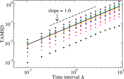
Figure 1: (Color online) TAMSD $\overline{(\delta x)^{2}}(\Delta,t)$ vs time interval $\Delta$ (log–log plot) for the one-dimensional system ($d=1$). Total measurement time $t$ is set as $t=10^{5}$ and other parameters as $\lambda=10^{-5},~{}\alpha=0.75$, and $c=1$. The TAMSDs are calculated for 17 different realizations of trajectories; a different symbol corresponds to a different realization. The solid line is their ensemble average.

PDF of time-averaged observables.—In this section, we derive the PDF of time-averaged observables $\overline{h}_{t}$. Because $\overline{h}_{t}$ and $N_{t}$ have the same PDF [Eq. (14)], we can study $N_{t}$ instead of $\overline{h}_{t}$. We have the following relations:

$$G(n;t) \equiv \mathrm{Prob\,}(N_{t}<n)=\mathrm{Prob\,}(T_{n}>t)$$ (15)

$$= \mathrm{Prob}\left(\sum_{k=1}^{n}\tau_{k}>t\right),$$

where $\mathrm{Prob\,}(\cdot)$ is the probability and $\tau_{k}$ is the trapping time between $(k-1)$-th and $k$-th jumps $(k=1,2,...)$. From Eq. (15), we obtain

$$G(n;t) = \int_{n^{-1/\alpha}t}^{\infty}d\tau~{}P_{\rm TL}(\tau,n^{1/\alpha}\lambda),$$ (16)

where we have used Eq. (7) and the fact that $\tau_{k}~{}(k=1,2,...)$ are mutually independent. Furthermore, we change the variables from $n$ to $z$ as $n=t^{\alpha}z$ with $t$ being set. Then, by using Eqs. (8), (15) and (16), we have

$$\mathrm{Prob}\left(\frac{N_{t}}{t^{\alpha}}<z\right) = -\frac{e^{c(t\lambda)^{\alpha}z}}{\alpha\pi}\sum_{k=1}^{\infty}\frac{\Gamma(k\alpha+1)}{k!k}$$ (17)

$$\times(-cz)^{k}\sin(\pi k\alpha)a_{k}(t),~{}~{}~{}~{}~{}$$

where $a_{k}(t)~{}(k=1,2,...)$ is defined by $a_{k}(t)\equiv\int_{0}^{1}d\tau e^{-t\lambda\tau^{-1/(\alpha k)}}.$ Differentiating Eq. (17) with respect to $z$, we have the PDF of $z=N_{t}/t^{\alpha}$:

$$f_{\lambda}(z;t) = -\frac{e^{c(t\lambda)^{\alpha}z}}{\alpha\pi}\sum_{k=1}^{\infty}\frac{\Gamma(k\alpha+1)}{k!}(-c)^{k}$$ (18)

$$\times\left[\frac{c(t\lambda)^{\alpha}z}{k}+1\right]z^{k-1}\sin(\pi k\alpha)a_{k}(t).~{}~{}~{}~{}~{}$$

Because of Eq. (11), Eq. (18) is the PDF of the time-averaged observables $\overline{h}_{t}t^{1-\alpha}/\left\langle H\right\rangle$ including the diffusion constant $D_{t}t^{1-\alpha}$ [Eq. (14)] as a special case. When $\lambda=0$, the PDF $f_{0}(z)$, which is the ML distribution Aaronson (1997); Akimoto and Miyaguchi (2010), is time-independent. Namely, the time-averaged observables are random variables even in the limit $t\to\infty$; this property is called the distributional ergodicity. On the other hand, when $\lambda>0$, the PDF tends to a delta function. Thus, the time-averages converge to constant values as is expected from the ordinary ergodicity. The PDF of $D_{t}$ is shown in Fig. 2 for three different measurement times $t$. It is clear that the PDF becomes narrower for a longer $t$. The analytical result given by Eq. (18) is also illustrated by the lines.

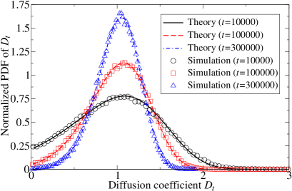
Figure 2: (Color online) The PDF of the diffusion coefficient $D_{t}$ for $d=1$. Each PDF is normalized so that its mean value equals unity. $D_{t}$ is calculated from TAMSD $\overline{(\delta x)^{2}}(\Delta,t)$ by least square fitting over the interval $0<\Delta<10$. The results for three different values of measurement times are presented: $t=10^{4}$ (circles), $10^{5}$ (squares), and $3\times 10^{5}$ (triangles). The other parameters are set as $\lambda=10^{-5},\alpha=0.75$, and $c=1$. The lines correspond to the theoretical predictions given by Eq. (18). Note that no adjustable parameters were used to obtain these figures.

Relative standard deviation.—Next, in order to quantify a deviation from the ordinary ergodicity, we study a relative standard deviation (RSD) of time-averaged observables $R(t)=\sqrt{\langle(\overline{h}_{t})^{2}\rangle_{c}}/\left\langle\overline{h}_{t}\right\rangle$, where $\left\langle\cdot\right\rangle$ is the ensemble average over trajectories and $\left\langle\cdot\right\rangle_{c}$ is the corresponding cumulant. If $R(t)\approx 0$, the system can be considered to be ergodic in the ordinary sense, whereas if $R(t)>0$, the system is not ergodic. To derive an analytical expression for $R(t)$, we take the Laplace transform of Eq (16) with respect to $t$:

$$\tilde{G}(n;s)=\frac{1-e^{-nc[(\lambda+s)^{\alpha}-\lambda^{\alpha}]}}{s},$$ (19)

where we have defined $\tilde{G}(n;s)$ as $\tilde{G}(n;s)\equiv\int_{0}^{\infty}dte^{-ts}G(n;t)$ and used Eq. (6). Next, we define a function $g(n;s)$ by $g(n;s):=\tilde{G}(n+1;s)-\tilde{G}(n;s)$. Then, by taking a (discrete) Laplace transform with respect to $n$, $\sum_{n=0}^{\infty}e^{-n\nu}g(n;s)\equiv\tilde{g}(\nu;s)$, we have

$$\tilde{g}(\nu;s)\simeq\frac{1}{s}\sum_{k=0}^{\infty}\left(-\frac{\nu}{c}\right)^{k}\left[(\lambda+s)^{\alpha}-\lambda^{\alpha}\right]^{-k},$$ (20)

where we used an approximation by assuming $s,\lambda\ll 1$. From Eq. (20), we can derive arbitrary order of moments of $N_{t}$. For example, the first moment $\left\langle N_{t}\right\rangle$ is given by

$$\left\langle N_{t}\right\rangle\simeq\left\{\begin{array}[]{ll}\displaystyle\frac{t^{\alpha}}{c\Gamma(\alpha+1)},&\hskip 8.5359ptt\ll 1/\lambda\\[7.11317pt] \displaystyle\frac{t}{c\lambda^{\alpha-1}\alpha}+\frac{1-\alpha}{2c\lambda^{\alpha}\alpha},&\hskip 8.5359ptt\gg 1/\lambda.\end{array}\right.$$ (23)

The ensemble-averaged mean square displacement (EAMSD) for CTRWs is known to be proportional to $\left\langle N_{t}\right\rangle$ Bouchaud and Georges (1990): $\left\langle(\delta\mbox{\boldmath$r$})^{2}\right\rangle(t)\sim\left\langle N_{t}\right\rangle$. Thus, the EAMSD of the present model shows transient subdiffusion, i.e., subdiffusion for short time scales and normal diffusion for long timescales Saxton (2007). Similarly, the second moment can be derived and we have the RSD for $N_{t}$ as follows:

$$\frac{\sqrt{\left\langle N_{t}^{2}\right\rangle_{c}}}{\left\langle N_{t}\right\rangle}\simeq\left\{\begin{array}[]{ll}\sqrt{\frac{2\Gamma^{2}(\alpha+1)}{\Gamma(2\alpha+1)}-1},&\hskip 8.5359ptt\ll 1/\lambda\\[0.0pt] (1-\alpha)^{1/2}\lambda^{-1/2}t^{-1/2},&\hskip 8.5359ptt\gg 1/\lambda.\end{array}\right.$$ (26)

Note that the RSDs for $\overline{h}_{t}$ and $D_{t}$ also follow the same relations, because they differ only in the scale factor [Eqs. (11) and (14)]. From these results, the crossover time $t_{c}$ between the distributional and ordinary ergodic regimes is given by

$$t_{c}=\frac{(1-\alpha)}{{2\Gamma^{2}(\alpha+1)}/{\Gamma(2\alpha+1)}-1}\lambda^{-1}.$$ (27)

As shown in Fig. 3, the RSD remains almost constant before the crossover time $t_{c}$, and starts to decay rapidly after the crossover. In Fig. 3, the RSD for the exponential trapping-time distribution which has the same mean trapping time $\left\langle\tau\right\rangle$ as the ETSD with $\lambda=10^{-6}$ is also shown by pluses. It is clear that the RSD for exponential distribution (pluses) decays much more rapidly than that for the ETSD (triangles).

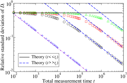
Figure 3: (Color online) RSD $\sqrt{\left\langle D_{t}^{2}\right\rangle_{c}}/\left\langle D_{t}\right\rangle$ vs total measurement time $t$ for $d=1$. $D_{t}$ is calculated from the TAMSD $\overline{(\delta x)^{2}}(\Delta,t)$ by least square fitting over the interval $0<\Delta<1$. Three different values of $\lambda$ are used: $\lambda=10^{-4}$ (circles), $10^{-5}$ (squares), and $10^{-6}$ (triangles), and $\alpha$ and $c$ are set as $\alpha=0.75$ and $c=1$, respectively. The lines correspond to the theoretical prediction given by Eq. (26); the solid line is the result for short time scales $t\ll t_{c}$, whereas the dashed lines are for long time scales $t\gg t_{c}$. The intersections of the solid and dashed lines correspond to the crossover times $t_{c}$ given by Eq. (27). The pluses are the RSD for the case of the exponential distribution $P(\tau)=\exp(\tau/\left\langle\tau\right\rangle)/\left\langle\tau\right\rangle$ with the same mean trapping time as the ETSD with $\lambda=10^{-6}$ (triangles): $\left\langle\tau\right\rangle=c\lambda^{\alpha-1}\alpha$. The dot-dashed line is a theoretical prediction for the exponential distribution: $R(t)=(c\alpha\lambda^{\alpha-1}/t)^{1/2}$.

Summary.—In this study, we have investigated the CTRWs with truncated $\alpha$-stable trapping times. The three main results are as follows: (i) We proved the distributional ergodicity for short measurement times; namely, the time averages of observables behave as random variables following the ML distribution. Moreover, we derived the PDF at arbitrary measurement times. It is very interesting to compare this analytical formula [Eq. (18)] with the results for lipid granules reported recently Jeon et al. (2011). We should also note that the limit distributions, the ML distribution for the case of observables studied in this paper, depends on the definition of observables Rebenshtok and Barkai (2007); *rebenshtok08; *akimoto08b. (ii) We found that the distributional ergodic behavior persists for a long time. In other words, the convergence to the ordinary ergodicity is remarkably slow in contrast to the case in which the trapping-time distribution is given by common distributions such as the exponential distribution. This indicates that, in real experiments, the time-averaged quantities could behave as random variables even for considerably long measurement times. (iii) We found a crossover from the distributional ergodicity in the short-time regime to the ordinary ergoodicity in the long-time regime. Finally, it is worth mentioning that these three main results are valid for a large class of observables. This implies that it is possible to choose an observable which is easy to measure experimentally. Then, the system parameters $\alpha$ and $\lambda$ can be experimentally determined by the short– and long–time behavior of the RSD $R(t)$ [Eq. (26)], respectively.

References

- Aaronson (1997) J. Aaronson, An Introduction to Infinite Ergodic Theory (American Mathematical Society, Province, 1997).
- Akimoto and Miyaguchi (2010) T. Akimoto and T. Miyaguchi, Phys. Rev. E 82, 030102 (2010).
- He et al. (2008) Y. He, S. Burov, R. Metzler, and E. Barkai, Phys. Rev. Lett. 101, 058101 (2008).
- Lubelski et al. (2008) A. Lubelski, I. M. Sokolov, and J. Klafter, Phys. Rev. Lett. 100, 250602 (2008).
- Miyaguchi and Akimoto (2011) T. Miyaguchi and T. Akimoto, Phys. Rev. E 83, 031926 (2011).
- Golding and Cox (2006) I. Golding and E. C. Cox, Phys. Rev. Lett. 96, 098102 (2006).
- Bronstein et al. (2009) I. Bronstein, Y. Israel, E. Kepten, S. Mai, Y. Shav-Tal, E. Barkai, and Y. Garini, Phys. Rev. Lett. 103, 018102 (2009).
- Wang et al. (2006) Y. M. Wang, R. H. Austin, and E. C. Cox, Phys. Rev. Lett. 97, 048302 (2006).
- Granéli et al. (2006) A. Granéli, C. C. Yeykal, R. B. Robertson, and E. C. Greene, Proc. Natl. Acad. Sci. U.S.A 103, 1221 (2006).
- Scher and Montroll (1975) H. Scher and E. W. Montroll, Phys. Rev. B 12, 2455 (1975).
- Young et al. (1989) W. Young, A. Pumir, and Y. Pomeau, Phys. Fluids A 1, 462 (1989).
- Song et al. (2010) C. Song, T. Koren, P. Wang, and A. Barabasi, Nat Phys 6, 818 (2010).
- Burov et al. (2011) S. Burov, J. Jeon, R. Metzler, and E. Barkai, Physical Chemistry Chemical Physics 13, 1800 (2011).
- Saxton (2007) M. J. Saxton, Biophys. J. 92, 1178 (2007).
- Bouchaud and Georges (1990) J. Bouchaud and A. Georges, Phys. Rep. 195, 127 (1990).
- Goychuk and Hänggi (2002) I. Goychuk and P. Hänggi, Proc. Natl. Acad. Sci. USA 99, 3552 (2002).
- Mantegna and Stanley (1994) R. N. Mantegna and H. E. Stanley, Phys. Rev. Lett. 73, 2946 (1994).
- Koponen (1995) I. Koponen, Phys. Rev. E 52, 1197 (1995).
- Nakao (2000) H. Nakao, Phys. Lett. A 266, 282 (2000).
- Gajda and Magdziarz (2010) J. Gajda and M. Magdziarz, Phys. Rev. E 82, 011117 (2010).
- Feller (1971) W. Feller, An Introduction to Probability Theory and its Applications, 2nd ed., Vol. II (Wiley, New York, 1971) Chap. 17.
- Burov et al. (2010) S. Burov, R. Metzler, and E. Barkai, Proc. Natl. Acad. Sci. U.S.A 107, 13228 (2010).
- Jeon et al. (2011) J.-H. Jeon, V. Tejedor, S. Burov, E. Barkai, C. Selhuber-Unkel, K. Berg-Sørensen, L. Oddershede, and R. Metzler, Phys. Rev. Lett. 106, 048103 (2011).
- Rebenshtok and Barkai (2007) A. Rebenshtok and E. Barkai, Phys. Rev. Lett. 99, 210601 (2007).
- Rebenshtok and Barkai (2008) A. Rebenshtok and E. Barkai, J. Stat. Phys. 133, 565 (2008).
- Akimoto (2008) T. Akimoto, ibid. 132, 171 (2008).