Damping of Electron Density Structures and Implications for Interstellar Scintillation

Abstract

The forms of electron density structures in kinetic Alfvén wave turbulence are studied in connection with scintillation. The focus is on small scales $L\sim 10^{8}-10^{10}$ cm where the Kinetic Alfvén wave (KAW) regime is active in the interstellar medium, principally within turbulent HII regions around bright stars. MHD turbulence converts to a KAW cascade, starting at 10 times the ion gyroradius and continuing to smaller scales. These scales are inferred to dominate scintillation in the theory of Boldyrev et al. (Boldyrev & Gwinn, 2003a, b, 2005; Boldyrev & Konigl, 2006). From numerical solutions of a decaying kinetic Alfvén wave turbulence model, structure morphology reveals two types of localized structures, filaments and sheets, and shows that they arise in different regimes of resistive and diffusive damping.  Minimal resistive damping yields localized current filaments that form out of Gaussian-distributed initial conditions.  When resistive damping is large relative to diffusive damping, sheet-like structures form.  In the filamentary regime, each filament is associated with a non-localized magnetic and density structure, circularly symmetric in cross section.  Density and magnetic fields have Gaussian statistics (as inferred from Gaussian-valued kurtosis) while density gradients are strongly non-Gaussian, more so than current.  This enhancement of non-Gaussian statistics in a derivative field is expected since gradient operations enhance small-scale fluctuations.  The enhancement of density gradient kurtosis over current kurtosis is not obvious, yet it suggests that modest fluctuation levels in electron density may yield large scintillation events during pulsar signal propagation in the interstellar medium.  In the sheet regime the same statistical observations hold, despite the absence of localized filamentary structures.  Probability density functions are constructed from statistical ensembles in both regimes, showing clear formation of long, highly non-Gaussian tails.

1 Introduction

Models of scintillation have a long history. Many (Lee & Jokipii, 1975a, b; Sutton, 1971) carry an implicit or explicit assumption of Gaussian statistics, applying to either the electron density field itself or its autocorrelation function (herein referred to as “Gaussian Models”). Lee & Jokipii (1975a) is a representative approach. The statistics of the two-point correlation function of the index of refraction $\epsilon(\mathbf{r})$, $A(\rho)=\int{dz^{\prime}\left<\epsilon(x,z)\epsilon(x+\rho,z^{\prime})\right>}$ determines, among other effects, the scaling of pulsar signal width $\tau$ with dispersion measure $DM$. The index of refraction $\epsilon(\mathbf{r})$ is a function of electron density fluctuation $n(\mathbf{r})$. The quantity $A(0)$ enters the equations, representing the second moment of the index of refraction. If the distribution function of $\epsilon(\mathbf{r})$ has no second-order moment (as in a Lévy distribution) $A(0)$ is undefined. The assumption of Gaussian statistics leads to a scaling of $\tau\sim DM^{2}$, which contradicts observation for pulsars with $DM>30$ cm^-3 pc. For these distant pulsars, $\tau\sim DM^{4}$ (Sutton, 1971; Boldyrev & Gwinn, 2003a, b).

To explain the anomalous $DM^{4}$ scaling, Sutton (1971) argued that the pulsar signal encounters strongly scattering turbulent regions for longer lines of sight, essentially arguing that the statistics, as sampled by a pulsar signal, are nonstationary. Considering the pulse shape in time, Williamson (1972, 1973, 1974) is unable to match observations with a Gaussian Model of scintillation unless the scattering region is confined to $1/4$ of the line of sight between the pulsar and Earth. These assumptions may have physical basis, since the ISM may not be statistically stationary, being composed of different regions with varying turbulence intensity (Boldyrev & Gwinn, 2005).

The theory of Boldyrev & Gwinn (2003a, b, 2005); Boldyrev & Konigl (2006) takes a different approach to explain the anomalous $DM^{4}$ scaling by considering Lévy statistics for the density difference (defined below). Lévy distributions are characterized by long tails with no defined moments greater than first-order [i.e., $A(0)$ is undefined for a Lévy distribution]. The theory recovers the $\tau\sim DM^{4}$ relation with a statistically stationary electron density field. This theory also does not constrain the scattering region to a fraction of the line-of-sight distance.

The determinant quantity in the theory of Boldyrev et al. is the density difference, $\Delta n=n(\mathbf{x}_{1},z)-n(\mathbf{x}_{2},z)$. According to this model, if the distribution function of $\Delta n$ has a power-law decay as $|\Delta n|\rightarrow\infty$ and has no second moment, then it is possible to recover the $\tau\sim DM^{4}$ scaling (Boldyrev & Gwinn, 2003b). Assuming sufficiently smooth fluctuations, $\Delta n$ can be expressed in terms of the density gradient, $\mathbf{\sigma}(z)$: $n(\mathbf{x}_{1})-n(\mathbf{x}_{2})\simeq\mathbf{\sigma}(z)\cdot(\mathbf{x}_{1}-\mathbf{x}_{2})$. Perhaps more directly, the density gradient enters the ray tracing equations [Eqns. (7) in Boldyrev & Gwinn (2003a)], and is seen to be central to determining the resultant pulsar signal shape and width. This formulation of a scintillation theory does not require the distribution of $\Delta n$ to be Gaussian or to have a second-order moment.

The notion that the density difference is characterized by a Lévy distribution is a constraint on dynamical models for electron density fluctuations in the ISM.  Consequently the question of how a Lévy distribution can arise in electron density fluctuations assumes considerable importance in understanding the ISM.

Previous work has laid the groundwork for answering this question. It has been established that electron density fluctuations associated with interstellar magnetic turbulence undergo a significant change in character near the scale $10\rho_{s}$, where $\rho_{s}$ is the ion sound gyroradius (Terry et al., 2001).  At larger scales, electron density is passively advected by the turbulent flow of an MHD cascade mediated by nonlinear shear Alfvén waves (Goldreich & Sridhar, 1995).  At smaller scales the electron density becomes compressive and the turbulent energy is carried into a cascade mediated by kinetic Alfvén waves (KAW) (Terry et al., 2001).  The KAW cascade brings electron density into equipartition with the magnetic field, allowing for a significant increase in amplitude.  The conversion to a KAW cascade has been observed in numerical solutions of the gyrokinetic equations (Howes et al., 2006), and is consistent with observations from solar wind turbulence (Harmon & Coles, 2005; Bale et al., 2005; Leamon et al., 1998).  Importantly, it puts large amplitude electron density fluctuations (and large amplitude density gradients) at the gyroradius scale ($\sim 10^{8}-10^{10}$ cm), a desirable set of conditions for pulsar scintillation (Boldyrev & Konigl, 2006).  It is therefore appropriate to consider whether large-amplitude non-Gaussian structures can arise in KAW turbulence.

This question has been partially answered in a study of current filament formation in decaying KAW turbulence (Terry & Smith, 2007, 2008).  In numerical solutions to a two-field model with broadband Gaussian initial conditions large amplitude current filaments spontaneously arose.  Each filament was associated with a large-amplitude electron density structure, circular in cross-section, that persisted in time.  These electron density structures were not as localized as the corresponding current filaments, but were coherent and not mixed by surrounding turbulence.  The observation of large amplitude current filaments is similar to the large-amplitude vortex filaments found in decaying 2D hydrodynamic turbulence (McWilliams, 1984).  Counterparts of such structures in 3D are predicted to be the dominant component for higher order structure functions (She & Leveque, 1994).

Terry & Smith (2007) proposed that a nonlinear refractive magnetic shear mechanism prevents the structures from mixing with turbulence.  Radial shear in the azimuthally directed magnetic field associated with each large-amplitude current filament decreases the radial correlation length of the turbulent eddies and enhances the decorrelation rate.  Eddies are unable to persist long enough to penetrate the shear boundary layer and disrupt the structure core.  The structure persistence mechanism allows large-amplitude fluctuations to persist for many eddy-turnover times.  As the turbulent decays these structures eventually dominate the statistics of the system.  The spatial structure of the density field associated with localized circularly symmetric current filaments was shown from analytical theory (Terry & Smith, 2007) to yield a Lévy-distributed density gradient field.  The kurtosis for the current field was significantly larger than the Gaussian-valued kurtosis of 3, indicating enhanced tails.  The electron density and magnetic field kurtosis values were not significantly greater than 3.  However, just as the current is non-Gaussian when the magnetic field is not, it is expected that numerical solutions should show non-Gaussian behavior for the density gradient.  In the present paper, density gradient statistics are measured and found to be non-Gaussian.  Rather than relying on kurtosis values alone, the probability density functions (PDFs) are computed from ensembles of numerical solutions, showing non-Gaussian PDFs for the density gradient field.

The previous studies of filament generation in KAW turbulence leave significant unanswered questions relating to structure morphology and its effect on scintillation.  It is well established that MHD turbulence admits structures that are both filament-like and sheet-like.  Can sheet-like structures arise in KAW turbulence?  If so, what are the conditions or parameters favoring one type of structure versus the other?  If sheet-like structures dominate in some circumstances, what are the statistics of the density gradient?  Can they be sufficiently non-Gaussian to be compatible with pulsar scintillation scaling? It is desirable to consider such questions prior to calculation of rf wave scattering properties in the density gradient fields obtained from numerical solutions.

In this paper, we show that both current filaments and current sheet structures naturally arise in numerical solutions of a decaying KAW turbulence model.  Each has a structure of the same type and at the same location in the electron density gradient.  These structures become prevalent as the numerical solutions progress in time, and each is associated with highly non-Gaussian PDFs. Moreover, we show that small-scale current filaments and current sheets, along with their associated density structures, are highly sensitive to the magnitude of resistive damping and diffusive damping of density fluctuations. Current filaments persist provided that resistivity $\eta$ is small; similarly, electron density fluctuations and gradients are diminished by large diffusive damping in the electron continuity equation. The latter results from collisions assuming density fluctuations are subject to a Fick’s law for diffusion. The magnitude of the resistivity affects (1) whether current filaments can become large in amplitude, (2) their spatial scale, and (3) the preponderance of these filaments as compared to sheets. The magnitude of the diffusive damping parameter, $\mu$, similarly influences the amplitude of density gradients and, to a lesser degree, influences the extent to which electron density structures are non-localized.

In the ISM resistive and diffusive damping become important near resistive scales. However, it is well known that collisionless damping effects are also present (Lysak & Lotko, 1996; Bale et al., 2005), and quite possibly dominate over collisional damping in larger scales near the ion Larmor radius. The collisional damping in the present work is understood as a heuristic approach that facilitates analysis of the effects of different damping regimes on the statistics of electron density fluctuations. By varying the ratio of resistive and diffusive damping we can, as suggested above, control the type of structure present in the turbulence. This allows us to isolate and study the statistics associated with each type of structure. It also allows us to assess and examine the type of environment conducive to formation of the structure. We consider regimes with large and small damping parameters, enabling us to explore damping effects on structure formation across a range from inertial to dissipative. Future work will address collisionless damping in greater detail.

1.1 Background Considerations for Structure Formation

The coherent structures observed in numerical solutions of decaying KAW turbulence, whether elongated sheets or localized filaments, are similar to structures observed in decaying MHD turbulence, as in Kinney & McWilliams (1995). In that work, the flow field initially gives rise to sheet-like structures. After selective decay of the velocity field energy, the system evolves into a state with sheets and filaments. During the merger of like-signed filaments, large-amplitude sheets arise, limited to the region between the merging filaments. These short-lived sheets exist in addition to the long-lived sheets not associated with the merger of filaments. In the two-field KAW system, however, there is no flow; the sheet and filament generation is due to a different mechanism, of which the filament generation has previously been discussed (Terry & Smith, 2007).

Other work (Biskamp & Welter, 1989; Politano et al., 1989) observed the spontaneous generation of current sheets and filaments in numerical solutions, with both Orszag-Tang vortex and randomized initial conditions. These 2D reduced MHD numerical solutions modeled the evolution of magnetic flux and vorticity with collisional dissipation coefficients $\eta$, the resistivity, and $\nu$, the kinematic viscosity. The magnetic Prandtl number, $\nu/\eta$, was set to unity. These systems are incompressible and not suitable for modeling the KAW system we consider here – they do however illustrate the ubiquity of current sheets and filaments, and serve as points of comparison. For Orszag-Tang-like initial conditions with large-scale flux tubes smooth in profile, current sheets are preferred at the interfaces between tubes. Tearing instabilities can give rise to filamentary current structures that persist for long times, but the large-scale and smoothness of flux tubes do not give rise to strong current filaments localized at the center of the tubes. To see this, consider a given flux tube, and model it as cylindrically symmetric and monotonically decreasing in $r$ with characteristic radial extent $a$,

$$\psi(r)=\psi_{0}\left(1-(\frac{r}{a})^{2}\right),$$ (1)

for $0\leq r\leq a$. The current is localized at the center with magnitude

$$J=-4\frac{\psi_{0}}{a^{2}}.$$ (2)

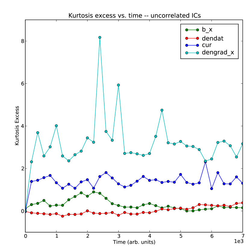
Figure 10: Kurtosis excess for a numerical solution with phase-uncorrelated initial conditions and $\eta/\mu=1$.

Thus flux tubes with large radial extent $a$ have a corresponding small current filament at their center. Hence, initial conditions dominated by a few large-scale flux tubes are not expected to have large amplitude current filaments at the flux tube centers, but favor current sheet formation and filaments associated with tearing instabilities in those sheet regions. At X points current sheet folding and filamentary structures can arise (see, e.g. Biskamp & Welter, 1989, Fig. 10), but these regions are small in area compared to the quiescent flux-tube regions. Note that if, instead of Orszag-Tang-like initial conditions, the initial state is random, one expects some regions with flux tubes that have $a$ small, and therefore a sizable current filament at the center.

Consider now the effect of comparatively large or small $\eta$. In the case of large $\eta$, the central region of a flux tube is smoothed by the collisional damping, thus having a strong suppressive effect on the amplitude of the current filament associated with such a flux tube. Large-amplitude current structures are localized to the interfaces between flux tubes. In the process of mergers between like-signed filaments (and repulsion between unlike-signed), large current sheets are generated at these interfaces, similar to the large-amplitude sheets generated in MHD turbulence during mergers (Kinney & McWilliams, 1995). For small $\eta$, relatively little suppression of isolated current filaments should occur; if these filaments are spatially separated owning to the buffer provided by their associated flux tube, they can be expected to survive a long time and only be disrupted upon the merger with another large-scale flux tube. Large $\eta$, then, allows current sheets to form at the boundaries between flux tubes while suppressing the spatially-separated current filaments at flux tube centers. Small $\eta$ allows interface sheets and spatially separated filaments to exist.

These simple arguments suggest that the evolution of the large-amplitude structures and their interaction with turbulence is thus strongly influenced by the damping parameters. As such, the magnitudes of the damping parameters are expected to affect the resultant pulsar scintillation scalings. The present paper considers the effect of variations of these damping parameters, $\eta$ and $\mu$. In the KAW model, the (unnormalized) resistivity takes the form $\eta=m_{e}\nu_{e}/ne^{2}$ and the density diffusion coefficient is $\mu=\rho_{e}^{2}\nu_{e}$, where $m_{e}$ is the electron mass, $\nu_{e}$ is the electron collision frequency, $n$ is the electron density, $e$ is the electron charge, and $\rho_{e}=v_{Te}/\omega_{ce}$, with $v_{Te}$ the electron thermal velocity, and $\omega_{ce}$ the electron gyrofrequency. The ratio of these terms, $c^{2}\eta/4\pi\mu=2/\beta$, where $\beta=8\pi nkT/B^{2}$ is the ratio of plasma to magnetic pressures. When we vary this ratio, as we will do in the numerical solutions presented here, we have in mind that we are representing regions of different $\beta$. However, as a practical matter in the numerical solutions, we must vary the damping parameters independently of the variation of $\beta$, since the kinetic Alfvén wave dynamics require a small $\beta$ to propagate. For the warm ionized medium, typical parameters are $T_{e}=8000\;\mathrm{K}$, $n=0.08\;\mathrm{cm}^{-3}$, $|B|=1.4\;\mu\mathrm{G}$, $\delta B=5.0\;\mu\mathrm{G}$ (Ferrière, 2001). With these parameters, the plasma $\beta$ formally ranges from $0.05-1.2$, spanning a range of plasma magnetization.

We present the results of numerical solutions of decaying KAW turbulence to ascertain the effect of different damping regimes on the statistics of the fields of interest, in particular the electron density and electron density gradient. In the $\eta\ll\mu$ regime (using normalized parameters), previous work (Craddock et al., 1991) had large-amplitude current filaments that were strongly localized with no discernible electron density structures ($\mu$ was large to preserve numerical stability). This regime is unable to preserve density structures or density gradients. The numerical solutions presented here have $\eta\sim\mu$ and $\eta\gg\mu$; in each limit the damping parameters are minimized so as to allow structure formation to occur, and are large enough to ensure numerical stability for the duration of each numerical solution. We investigate the statistics of both filaments and sheets in the context of scintillation in the warm ionized medium.

The paper is arranged as follows: section 2 gives an overview of the KAW model and normalizations, its regime of validity, and its dispersion relation. Section 3 discusses the numerical method used and the field initializations. The negligible effect of initial cross-correlation between fields is discussed. Results for the two damping regimes are given in section 4, where the type of structures that form, whether sheets-and-filaments or predominantly sheets, are seen to be dependent on the values of $\eta$ and $\mu$. PDFs from ensemble numerical solutions are presented in section 5, illustrating the strongly non-Gaussian statistics in the electron density gradient field for both the $\eta\sim\mu$ and $\eta\gg\mu$ regimes. This suggests that non-Gaussian electron-density gradients are robust to variation in $\eta$, as long as the overall damping in the continuity equation is not too large. Some discussions regarding the limitations of numerical approximation for this work and possible enhancements–particularly a model that addresses driven KAW turbulence–are given in concluding remarks.

2 Kinetic Alfvén Wave Model

The kinetic Alfvén wave (KAW) model used in this paper is the same model used in theories of pulsar scintillation through the ISM (Terry & Smith, 2007, 2008) and in earlier work (Craddock et al., 1991). It is a reduced, two-field, small-scale limit of a more general reduced three-field MHD system (Hazeltine, 1993; Rahman & Wieland, 1983; Fernandez & Terry, 1997) that accounts for electron dynamics parallel to the magnetic field.

The 3-field model applies to large and small-scale fluctuations as compared to $\rho_{s}$, the ion gyroradius evaluated at the electron temperature. In large-scale strong turbulence magnetic and kinetic fluctuations are in equipartition, with electron density passively advected. In the limit of small spatial scales ($\leq 10\rho_{s}$) the roles of kinetic and internal fluctuations are reversed – magnetic fluctuations are in equipartition with density fluctuations, and kinetic energy experiences a go-it-alone cascade without participating in the magnetic-internal energy interaction. The shear-Alfvén physics at large scale is supplanted by kinetic-Alfvén physics at small scale (Terry et al., 2001).

In the Boldyrev et al. theory, the length scales that dominate scintillation for pulsars with $DM>30\;\mathrm{pc}\;\mathrm{cm}^{-3}$ are small, around $10^{8}-10^{10}\;\mathrm{cm}$. This motivates our focus on the small-scale regime of the more general 3-field system. The dominant interactions are between magnetic and internal fluctuations, via kinetic Alfvén waves. In these waves, electron density gradients along the magnetic field act on an inductive electric field in Ohm’s law. The electron continuity equation serves to close the system. The normalized equations are

$$\partial_{t}\psi=\nabla_{\|}n+\eta_{0}J-\eta_{2}\nabla^{2}J,$$ (3)

$$\partial_{t}n=-\nabla_{\|}J+\mu_{0}\nabla^{2}n-\mu_{2}\nabla^{2}\nabla^{2}n,$$ (4)

$$\nabla_{\|}=\partial_{z}+\nabla\psi\times\mathrm{z}\cdot\nabla,$$ (5)

$$J=\nabla^{2}\psi,$$ (6)

with $\psi=(C_{s}/c)eA_{z}/T_{e}$, the normalized parallel component of the vector potential and $n=(C_{s}/V_{A})\tilde{n}/n_{0}$ the normalized electron density. The normalized resistivity is $\eta_{0}=(c^{2}/4\pi V_{A}\rho_{s})\eta_{sp}$, with $\eta_{sp}$ the Spitzer resistivity, given in the introduction. The normalized diffusivity is $\mu=\rho_{e}^{2}\nu_{e}/\rho_{s}V_{A}$. The time and space normalizations are $\tau_{A}=\rho_{s}/V_{A}$ and $\rho_{s}=C_{s}/\Omega_{i}$. Here $C_{s}=(T_{e}/m_{i})^{1/2}$ is the ion acoustic velocity, $V_{A}=B/(4\pi m_{i}n_{0})^{1/2}$ is the Alfvén speed, and $\Omega_{i}=eB/m_{i}c$ is the ion gyrofrequency. Electron density diffusion is presumed to follow Fick’s law; more detailed damping would necessarily consider kinetic effects and cyclotron resonances. The $\eta_{2}$ and $\mu_{2}$ terms (hyper-resistivity and hyper-diffusivity) are introduced to mitigate large-scale Fourier-mode damping by the linear diffusive terms. Throughout the remainder of the paper, we drop the $2$ subscript from $\eta_{2}$ and $\mu_{2}$ and refer to the hyper-dissipative terms as $\eta$ and $\mu$.

Three ideal invariants exist: total energy $E=\int d^{2}x[(\nabla\psi)^{2}+\alpha n^{2}]$; flux $F=\int d^{2}x\;\psi^{2}$ and cross-correlation $H_{c}=\int d^{2}x\;n\psi$. Energy cascades to small scale (large $k$) while the flux and cross-correlation undergo an inverse cascade to large-scale (small $k$) (Fernandez & Terry, 1997). The inverse cascades require the initialized spectrum to peak at $k_{0}\neq 0$ to allow for buildup of magnetic flux at large-scales for later times.

Linearizing the system yields a (dimensional) dispersion relation $\omega=V_{A}k_{z}k_{\perp}\rho_{s}$. The mode combines perpendicular oscillation associated with a finite gyroradius with fluctuations along a mean field ($z$-direction). The oscillating quantities are magnetic field and density, out of phase by $\pi/2$ radians.

In the limit of strong mean field, quantities along the mean field ($z$-direction) equilibrate quickly, which allows $\partial/\partial z\rightarrow 0$, or $k_{z}\rightarrow 0$. Kinetic Alfvén waves still propagate, as long as there are a broad range of scales that are excited, as in fully developed turbulence. As $k_{z}\rightarrow 0$, all gradients are localized to the plane perpendicular to the mean field. Presuming a large-scale fluctuation at characteristic wavenumber $\mathbf{k}_{0}$, smaller-scale fluctuations propagate linearly along this larger-scale fluctuation so long as their characteristic scale $k$ satisfies $k\gg k_{0}$. In this reduced, two dimensional system, the above dispersion relation is modified to be $\omega=V_{A}(\mathbf{b}_{k_{0}}\cdot\mathbf{k}/B)k\rho_{s}$ which is still Alfvénic but with respect to a perturbed large-scale amplitude perpendicular to the mean field. Relaxing the scale separation criterion yields $\omega\propto k^{2}$ for the general case.

3 Numerical Solution Method

We evolve Eqs. (3) and (4) in a 2D periodic box, size $[2\pi]\times[2\pi]$ on a mesh of resolution $512\times 512$. The $\psi$ and $n$ scalar fields are evolved in the Fourier domain, with the nonlinearities advanced pseudospectrally and with full $2/3$ dealiasing in each dimension (Orszag, 1971). The diffusive and resistive terms normally introduce stiffness into the equations; using an integrating factor removes any stability constraints stemming from these terms. Following the scheme outlined in Canuto et al. (1990), we start with the semi-discrete formulation of Eqs. (3) and (4):

$$\frac{d\psi_{k}}{dt}=-\eta k^{4}\psi_{k}+\mathcal{F}\left[\nabla_{\|}n\right]$$ (7)

$$\frac{dn_{k}}{dt}=-\mu k^{4}n_{k}-\mathcal{F}\left[\nabla_{\|}J\right],$$ (8)

where $\mathcal{F}[\cdot]$ denotes the discrete Fourier transform. We do not explicitly expand the nonlinear terms as they will be integrated separately. The hyper-damping terms (proportional to $k^{4}$) are included above. Damping terms corresponding to the Laplacian operator (proportional to $k^{2}$) are not included in this section for clarity, but are trivial to incorporate. Equations 7 and 8 can be put in the form

$$\frac{d}{dt}\left[e^{\eta k^{4}t}\psi_{k}\right]=e^{\eta k^{4}t}\mathcal{F}\left[\nabla_{\|}n\right]$$ (9)

$$\frac{d}{dt}\left[e^{\mu k^{4}t}n_{k}\right]=-e^{\mu k^{4}t}\mathcal{F}\left[\nabla_{\|}J\right].$$ (10)

A second-order Runge-Kutta scheme for the $\psi_{k}$ difference equation is

$$\psi_{k}^{m+1/2}=e^{-\eta k^{4}\Delta t/2}\left[\psi_{k}^{m}+\Delta t/2\mathcal{F}\left[\nabla_{\|}n^{m}\right]\right]$$ (11)

$$\psi_{k}^{m+1}=e^{-\eta k^{4}\Delta t}\left[\psi_{k}^{m+1/2}+\Delta t\mathcal{F}\left[\nabla_{\|}n^{m+1/2}\right]\right]$$ (12)

with a similar form for the $n_{k}$ scheme.

3.1 Initial conditions

The $\psi_{k}$ and $n_{k}$ fields are initialized such that the energy spectra are broad-band with a peak near $k_{0}\sim 6-10$ and a power law spectrum for $k>k_{0}$. The falloff in $k$ is predicted to be $k^{-2}$ for small-scale turbulence. Craddock et al. (1991) use $k^{-3}$, between the current-sheet limit of $k^{-4}$ and the kinetic-Alfvén wave strong-turbulence limit of $k^{-2}$. The numerical solutions considered here have either $k^{-2}$ or $k^{-3}$. The only qualitative difference between the two spectra is the scale at which structures initially form. The $k^{-2}$ spectra has more energy at smaller scales, leading to smaller characteristic structure size. After a few tens of Alfvén times these smaller-scale structures merge and the system resembles the initial $k^{-3}$ spectra.

The $n_{k}$ and $\psi_{k}$ phases can be either cross-correlated or uncorrelated. By cross-correlated we mean that the phase angle for each Fourier component of the $n_{k}$ and $\psi_{k}$ fields are equal. In general,

$$n_{k}=|A_{k}|e^{i\theta_{1}},\qquad\psi_{k}=|B_{k}|e^{i\theta_{2}},$$ (13)

where $|A_{k}|$ and $|B_{k}|$ are the Fourier component’s amplitude, set according to the spectrum power-law. For cross-correlated initial conditions, $\theta_{1}=\theta_{2}$ for all $\mathbf{k}$ at the initial time. For uncorrelated initialization, there is no phase relation between corresponding Fourier components of the $n_{k}$ and $\psi_{k}$ fields.

Craddock et al. (1991) focused on the formation and longevity of current filaments in a turbulent KAW system. To preserve small-scale structure in the current filaments, these numerical solutions set $\eta=0$ and had $\mu\sim 10^{-3}$, with a resolution of $128\times 128$, corresponding to a $k_{max}$ of 44. Large-amplitude density structures that would have arisen were damped to preserve numerical stability up to an advective instability time of a few hundred Alfvén times, for the parameter values therein. The numerical solutions presented here explore a range of parameter values for $\eta$ and $\mu$. They make use of hyper-diffusivity and hyper-resistivity of appropriate strengths to preserve structures in $n$, $B$ and $J$. An advective instability is excited after $\sim 10^{2}$ Alfvén times if resistive damping is negligible. The $\eta=0$ solutions–not presented here due to their poor resolution of small-scale structures–see large-amplitude current filaments arise, but they can be poorly resolved at this grid spacing. With no resistivity, the finite number of Fourier modes cannot resolve arbitrarily small structures without Gibbs phenomena resulting and distorting the current field.

We have found through experience that small hyper-resistivity and small hyper-diffusivity preserve large-amplitude density structures and their spatial correlation with the magnetic and current structures, while preventing the distortion resulting from poorly-resolved current sheets and filaments. They allow the numerical solutions to run for arbitrarily long times, and the effects of structure mergers become apparent. These occur on a longer timescale than the slowest eddy turnover times. The results presented here will consider two regimes of parameter values, the $\eta\approx\mu$ and $\eta\gg\mu$ regimes. The effect of cross-correlated and uncorrelated initial conditions will be addressed presently.

4 Results

It is of interest to examine whether cross-correlated or uncorrelated initial conditions affect the long-term behavior of the system. Two representative numerical solutions are presented here that reveal the system’s tendency to form spatially-correlated structures in electron density and current regardless of initial phase correlations. This study establishes the robustness of density structure formation in KAW turbulence and lends confidence that such structures should exist in the ISM under varying circumstances. The first numerical solution has cross-correlated initial conditions between the $n$ and $\psi$ fields; the second, uncorrelated. Damping parameters $\eta$ and $\mu$ are equal and large enough to ensure numerical stability while preserving structures in density, current and magnetic fields. These examples also serve to explore the intermediate $\eta/\mu$ regime.

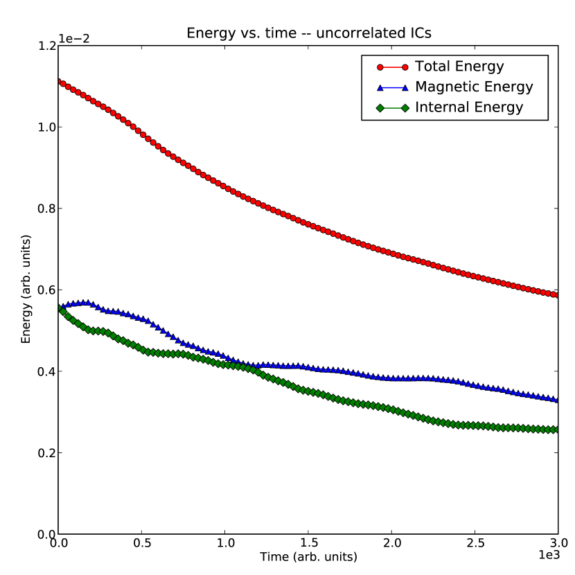
Figure 2: Energy vs. time for uncorrelated initial conditions. Total energy is monotonically decreasing with time, and magnetic and internal energies remain in rough equipartition.

The energy vs. time history for both numerical solutions are given in Figs. 1 and 2. Total energy is a monotonically decreasing function of time. The magnetic and internal energies remain in overall equipartition throughout the numerical solutions. Magnetic energy increases at the expense of internal energy and vice versa. This energy interchange is consistent with KAW dynamics and overall energy conservation in the absence of resistive or diffusive terms. The exchange is crucial in routinely producing large amplitude density fluctuations in this two-field model of nonlinearly interacting KAWs.

The total energy decay rates for the uncorrelated and correlated initial conditions in Figs. 1 and 2 differ, with the latter decaying more strongly than the former. The damping parameters are identical for the two numerical solutions, and the decay-rate difference remains under varying randomization seeds. The magnitudes of the nonlinear terms during the span of a numerical solution in Eqs. (3) and (4) for uncorrelated initial conditions are consistently larger than those of correlated initial conditions by a factor of 5. This difference lasts until 2500 Alfvén times, after which the decay rates are roughly equal in magnitude. The steeper energy decay during the run of numerical solutions with uncorrelated initial conditions (Fig. 2) suggests that the enhancement of the uncorrelated nonlinearities transports energy to higher $k$ (smaller scale) more readily than the nonlinearities in the correlated case. Relatively more energy in higher $k$ enhances the energy decay rate as the linear damping terms dissipate more energy from the system. The initial configuration, whether correlated or uncorrelated, is seen to have an effect on the long-term energy evolution for these decaying numerical solutions. It will be shown below, however, that the correlation does not significantly affect the statistics of the resulting fields.

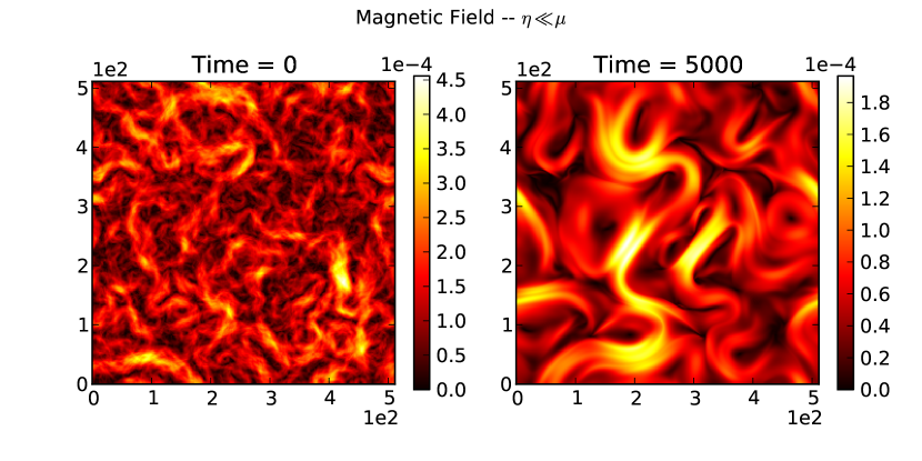
Figure 4: Contours of $|\mathrm{B}|$ for various times in a numerical solution with correlated initial conditions.

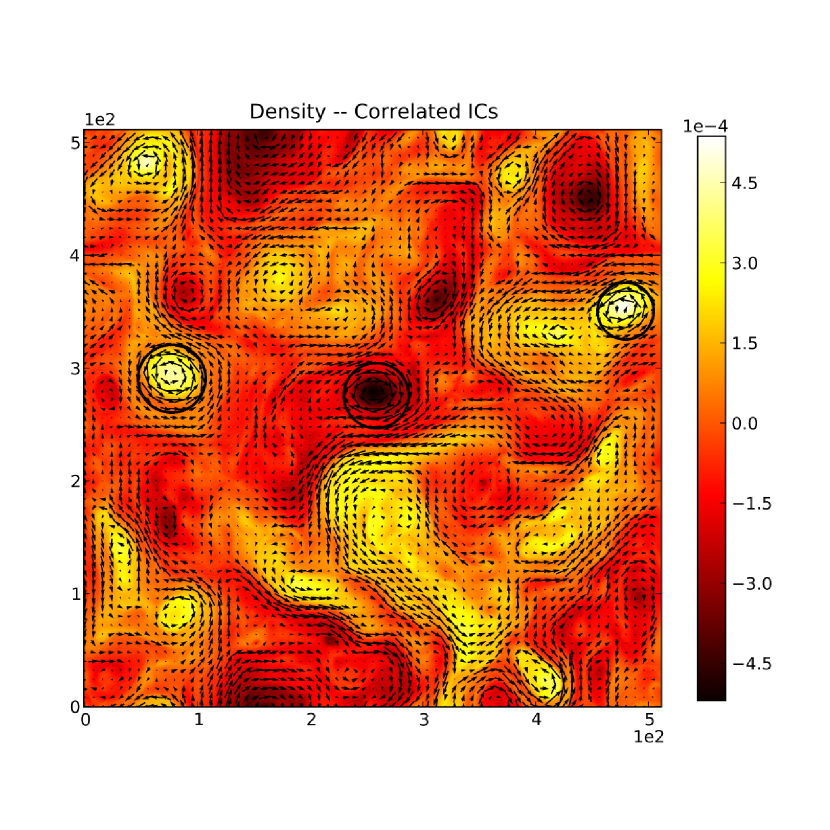
Figure 5: Contour plot of $n$ with $\mathbf{B}$ vectors overlaid. The positive, circularly-symmetric density structures correspond to counterclockwise-directed $\mathbf{B}$ structures; the opposite holds for negative circularly-symmetric density structures. These spatial correlations are to be expected for correlated initial conditions.

For cross-correlated initial conditions, we expect there to be a strong spatial relation between current, magnetic field and density structures through time. Figs. 3 and 4 show the $n$ and $|\mathrm{B}|$ contours at various times. For the latest time contour, the spatial structure alignment is evident. Further, in Fig. 5, the circular magnetic field structures (magnetic field direction and intensity indicated by arrow overlays) align with the large-amplitude density fluctuations. The correlation is evident once one notices that every positive-valued circular $n$ structure corresponds to counterclockwise-oriented magnetic field, and vice versa. Fig. 5 is at a normalized time of 5000 Alfvén times, defined in terms of the large $\mathrm{B}_{0}$. The system preserves the spatial structure correlation indefinitely, even after structure mergers.

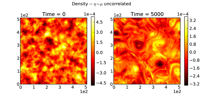
Figure 6: Contours of $n$ for various times in a numerical solution with uncorrelated initial conditions.

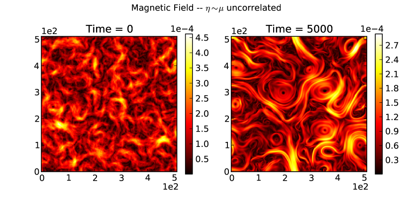
Figure 7: Contours of $|\mathrm{B}|$ for various times in a numerical solution with uncorrelated initial conditions.

The second representative numerical solution is one with uncorrelated initial conditions. Contour plots of density and $|\mathrm{B}|$ are given in Figs. 6 and 7, respectively. It is noteworthy that, similar to the cross-correlated initial conditions, spatially correlated density and magnetic field structures are discernible at the latest time contour.

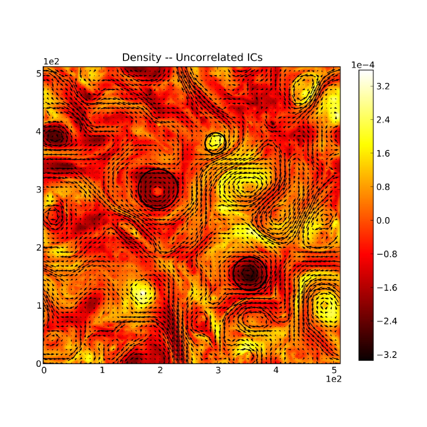
Figure 8: Contour plot of $n$ with $\mathbf{B}$ vectors overlaid for a numerical solution with initially uncorrelated initial conditions. The positive, circularly-symmetric density structures correspond to magnetic field structures, although the sense (clockwise or counterclockwise) of the magnetic field structure does not correlate with the sign of the density structures. Circled in black are symmetric structures that display a high degree of spatial correlation. The circle gives an approximate indication of the separatrix for the structure.

In Fig. 8 the circular density structures correspond to circular magnetic structures. Unlike Fig. 5 the positive density structures may correspond to clockwise or counterclockwise directed magnetic field structures. This serves to illustrate that, although the initial conditions have no phase relation between fields, after many Alfvén times circular density structures spatially correlate with magnetic field structures and persist for later times.

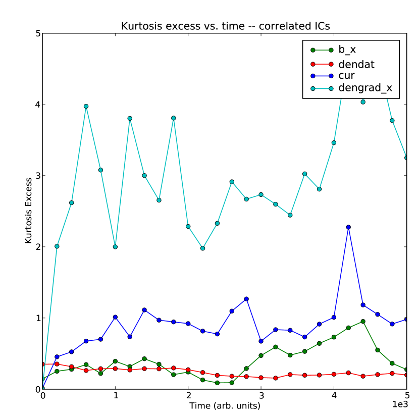
Figure 9: Kurtosis excess for a numerical solution with phase-correlated initial conditions and $\eta/\mu=1$.

The kurtosis excess as a function of time, defined as $K(\Xi)=\left<\Xi^{4}\right>/\sigma_{\Xi}^{4}-3$, is shown in Figs. 9 and 10 for correlated and uncorrelated initial conditions, respectively. Positive $K$ indicates a greater fraction of the distribution is in the tails as compared to a best-fit Gaussian. These figures indicate that the non-Gaussian statistics for the fields of interest are independent of initial correlation in the fields. In particular, the density gradients, $|\nabla n|$, are significantly non-Gaussian as compared to the current. Because scintillation is tied to density gradients, this situation is expected to favor the scaling inferred from pulsar signals.

The tendency of density structures to align with magnetic field structures regardless of initial conditions indicates that the initial conditions are representative of fully-developed turbulence. After a small number of Alfvén times the memory of the initial state is removed as the KAW interaction sets up a consistent phase relation between the fluctuations in the magnetic and density fields. Previous work (Terry & Smith, 2007) presented a mechanism whereby these spatially correlated structures can be preserved via shear in the periphery of the structures. The above figures indicate that this mechanism is at play even in cases where the initial phase relations are uncorrelated.

In the damping regime presented above, circularly symmetric structures in density, current and magnetic fields readily form and persist for many Alfvén times, until disrupted by mergers with other structures of similar amplitude. It is possible to define, for each circular structure, an effective separatrix that distinguishes it from surrounding turbulence and large-amplitude “sheets” that exist between structures. [see, e.g., the magnetic field contours at later times in Fig. 7.] The density field has significant gradients in both the regions surrounding the structure and within the structures themselves. The ability to separate these circular structures from the background sheets and turbulence is determined by the magnitudes – relative and absolute – of the damping parameters. Larger damping values erode the small-spatial-scale structures to a greater extent and, if large enough, disrupt the structure persistence mechanism that, for a fixed diameter, depends on a sufficiently large amplitude current filament to generate a sufficiently large radially sheared magnetic field.

The preceding results were for a damping regime where $\eta/\mu\sim 1$, an intermediate regime. Numerical solutions with $\mu=0$ and $\eta$ small explore the regime where $\eta/\mu\rightarrow 0$. In this regime, which is opposite the regime used in Craddock et al., circularly symmetric current and magnetic structures are not as prevalent, rather, sheet-like structures dominate the large amplitude fluctuations. Current and magnetic field gradients are strongly damped, and the characteristic length scales in these fields are larger.

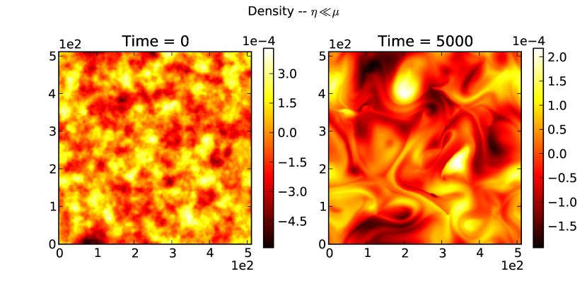
Figure 11: Electron density contour visualization with diffusive damping parameter $\mu=0$ for various times.

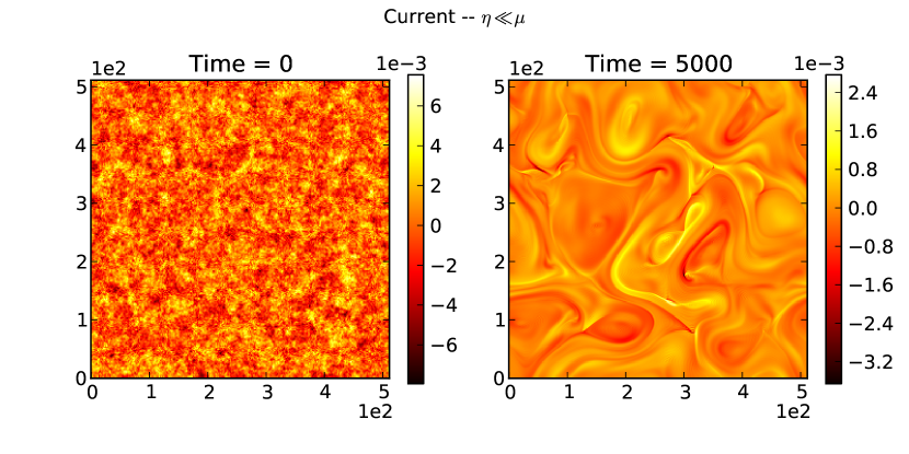
Figure 12: Current density contour visualization with diffusive damping parameter $\mu=0$ for various times.

Contours of density for a numerical solution with $\mu=0$ are shown in Fig. 11. Visual comparison with contours for runs with smaller damping parameters (Fig. 6, where $\eta=\mu$) indicate a preponderance of sheets in the $\mu=0$ case, at the expense of circularly-symmetric structures as seen above. All damping is in $\eta$; any current filament that would otherwise form is unable to preserve its small-scale, large amplitude characteristics before being resistively damped. Inspection of the current and $|B|$ contours for the same numerical solution [Figs. 12 and 13] reveal broader profiles and relatively few circular current and magnetic field structures with a well-defined separatrix as in the small $\eta$ case. Since there is no diffusive damping, gradients in electron density are able to persist, and electron density structures generally follow the same structures in the current and magnetic fields.

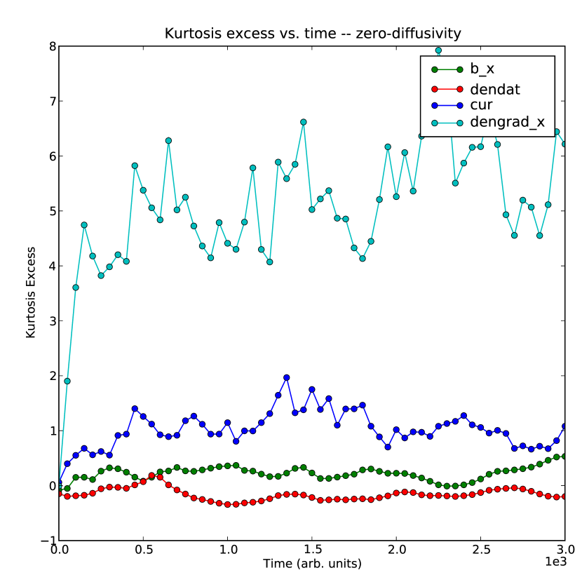
Figure 14: Kurtosis excess for a numerical solution with diffusive parameter $\mu=0$. Density gradient kurtosis remains greater than current kurtosis for the duration of the numerical solution.

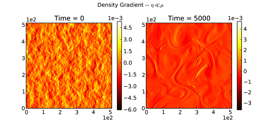
Figure 15: Electron density gradient ($x$ direction) contour visualization with diffusive damping $\mu=0$ for various times.

Kurtosis excess measurements for the $\mu=0$ numerical solutions yield mean values consistent with the $\eta=\mu$ numerical solutions, as seen in Fig. 14. Magnetic field strength and electron density statistics are predominantly Gaussian, with current statistics and density gradient statistics each non-Gaussian. Perhaps not as remarkable in this case, the density gradient kurtosis excess is again seen to be greater than the current kurtosis excess – this is anticipated since the dominant damping of density gradients is turned off. With fewer filamentary current structures, however, the mechanism proposed in Terry & Smith (2007) is not likely to be at play in this case, since few large-amplitude filamentary current structures exist. Sheets, evident in the density gradients in Fig. 15 and in the current in Fig. 12 are the dominant large-amplitude structures and determine the extent to which the density gradients have non-Gaussian statistics. The current and density sheets are well correlated spatially. The largest sheets can extend through the entire domain, and evolve on a longer timescale than the turbulence. Sheets exist at the interface between large-scale flux tubes, and are regions of large magnetic shear, giving rise to reconnection events. With $\eta$ relatively large, the sheets evolve on timescales shorter than the structure persistence timescale associated with the long-lived flux tubes.

Sheets and filaments are the dominant large-amplitude, long timescale structures that arise in the KAW system. Filaments arise and persist as long as $\eta$ is small, with their amplitude and statistical influence diminished as $\eta$ increases. Sheets exist in both regimes, becoming the sole large-scale structure in the large $\eta$ regime. Density gradients are consistently non-Gaussian in both regimes as long as $\mu$ is small, although the density structures are different in both regimes. Density gradient sheets arise in the large $\eta$ regime and these density gradient sheets are large enough to yield non-Gaussian statistics.

5 Ensemble Statistics and PDFs

To explicitly analyze the extent to which the decaying KAW system develops non-Gaussian statistics, ensemble runs were performed for both the $\eta/\mu\sim 1$ and $\eta/\mu\ll 1$ regimes, and PDFs of the fields were generated.

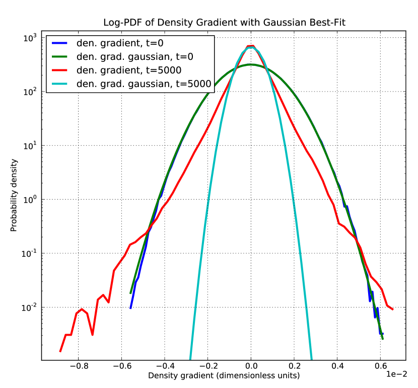
Figure 16: log-PDF of density gradients for an ensemble of numerical solutions with $\eta/\mu=1$ at $t=0$ and $t=5000$. The density gradient field at $t=0$ is Gaussian distributed, while for $t=5000$ the gradients are enhanced in the tails, and deviate from a Gaussian. A best-fit Gaussian for each PDF is plotted for comparison.

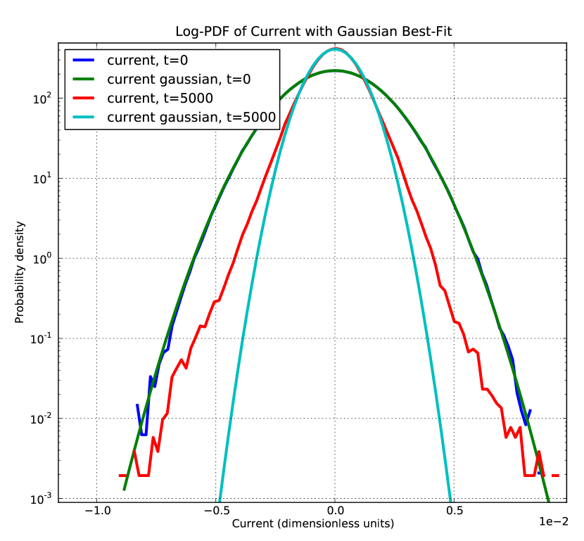
Figure 17: log-PDF of current for an ensemble of numerical solutions with $\eta/\mu=1$ at $t=0$ and $t=5000$. The current at $t=0$ is Gaussian distributed. For $t=5000$ the current is non-Gaussian. Unlike the density gradient, the current is not enhanced in the tails of the PDF for later times relative to its initial Gaussian envelope.

For the $\eta/\mu\sim 1$ regime, 10 numerical solutions were evolved with identical parameters but for different randomization seeds. In this case $\eta=\mu$ and both damping parameters have minimal values to ensure numerical stability. The fields were initially phase-uncorrelated. The density gradient ensemble PDF for two times in the solution results is shown in Fig. 16. Density gradients are Gaussian distributed initially. Many Alfvén times into the numerical solution the statistics are non-Gaussian with long tails. These PDFs are consistent with the time histories of density gradient kurtosis excess as shown above. The distribution tail extends beyond 15 standard deviations, almost 90 orders of magnitude above a Gaussian best-fit distribution. Similar behavior is seen in the current PDFs – initially Gaussian distributed tending to strongly non-Gaussian statistics with long tails for later times. Fig. 17 is the current PDF at an advanced time into the numerical solution. It is to be noted that the density gradient PDF has longer tails at higher amplitude than does the current PDF. One would expect these to be in rough agreement, since the underlying density and magnetic fields have comparable PDFs that remain Gaussian distributed throughout the numerical solution. The discrepancy between the density gradient and current PDFs suggests a process that enhances density derivatives above magnetic field derivatives. Future work is required to explore causes of this enhancement. This result is significant for pulsar scintillation, which is most sensitive to density gradients. Although interstellar turbulence is magnetic in nature, the KAW regime has the benefit of fluctuation equipartition between $n$ and $B$. The density gradient, however, is more non-Gaussian than the magnetic component, suggesting that this type of turbulence is specially endowed to produce the type of scintillation scaling observed with pulsar signals.

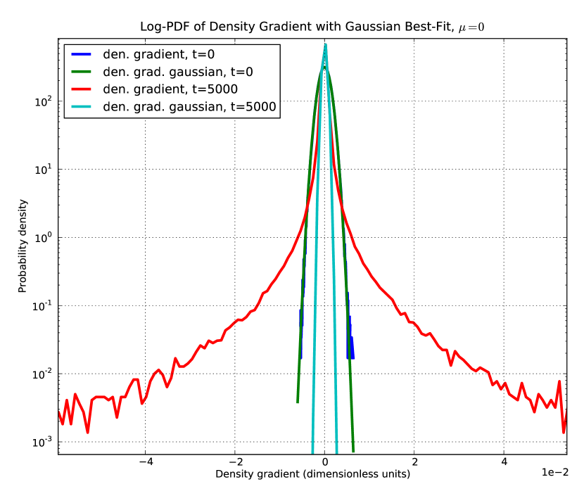
Figure 18: Log-PDF of density gradient for an ensemble of numerical solutions with $\mu=0$ at $t=0$ and $t=5000$. The density gradient field at $t=0$ is Gaussian distributed, while for $t=5000$ the gradients are enhanced in the tails, and deviate from a Gaussian. A best-fit Gaussian for each PDF is plotted for comparison.

Ensemble runs for the $\eta/\mu\ll 1$ regime yield distributions similar to the $\eta/\mu\sim 1$ regime in all fields. The ensemble PDF for two times is shown in Fig. 18. The initial density gradient PDF is Gaussian distributed. For later times long tails are evident and consistent with the kurtosis excess measurements as presented above for the $\mu=0$ case. The density gradient distribution has longer tails at higher amplitude than the current distribution; the overall distributions are similar to those for the $\eta/\mu\sim 1$ regime, despite the absence of filamentary structures and the presence of sheets. The strongly non-Gaussian statistics are insensitive to the damping regime, provided that the diffusion coefficient is small enough to allow density gradients to persist.

6 Discussion

Using the normalizations for Eqs. (3) and (4) and using $B=1.4\mu$G, $n=0.08$ cm^-3 and $T_{e}=1$ eV, $\eta_{norm}$, the normalized Spitzer resistivity, is $2.4\times 10^{-7}$ and $\mu_{norm}$, the normalized collisional diffusivity, is $1.9\times 10^{-7}$. For a resolution of $512^{2}$, these damping values are unable to keep the system numerically stable. The threshold for stability requires the simulation $\eta$ to be greater than $5\times 10^{-6}$, which is almost within an order of magnitude of the ISM value. The numerical solutions presented here, while motivated by the pulsar signal width scalings, more generally characterize the current and density gradient PDFs when the damping parameters are varied. We would expect the density gradients to be non-Gaussian when using parameters that correspond to the ISM. Future work will address the pulsar width scaling using electron density fields from the numerical solution.

The non-Gaussian distributions presented here are strongly tied to the fact that the system is decaying and that circular intermittent structures are preserved from nonlinear interaction. One can show that, in the KAW system, circularly symmetric structures (or filaments) are force free in Eqs. (3) and (4), i.e., the nonlinearity is zero. Once a large-amplitude structure becomes sufficiently circularly symmetric and is able to preserve itself from background turbulence via the shear mechanism, that structure is expected to persist on long timescales relative to the turbulence. Structure mergers will lead to a time-asymptotic state with two oppositely-signed current structures and no turbulence. As structures merge, kurtosis excess increases until the system reaches a final two-filament state, which would have a strongly non-Gaussian distribution and large kurtosis excess.

If the system were driven, energy input at large scales would replenish large-amplitude fluctuations. New structures would arise from large amplitude regions whenever the radial magnetic field shear were large enough to preserve the structure from interaction with turbulence. One could define a structure-replenishing rate from the driving terms that would depend on the energy injection rate and scale of injection. The non-Gaussian measures for a driven system would be characterized by a competition between the creation of new structures through the injection of energy at large scales and the annihilation of structures by mergers or by erosion from continuously replenished small-scale turbulence. If erosion effects dominate, the kurtosis excess is maintained at Gaussian values, diminishing the PDF tails relative to a Lévy distribution. If replenishing effects dominate, however, the enhancement of the tails of the density gradient PDF may be observed in a driven system as it is observed in the present decaying system. We note that structure function scaling in hydrodynamic turbulence is consistent with the replenishing effects becoming more dominant relative to erosion effects as scales become smaller, i.e., the turbulence is more intermittent at smaller scales. The large range of scales in interstellar turbulence and the conversion of MHD fluctuations to kinetic Alfvén fluctuations at small scales both support the notion that the structures of the decaying system are relevant to interstellar turbulence at the scales of KAW excitations. This scenario is consistent with arguments suggested by Harmon & Coles (2005). They propose a turbulent cascade in the solar wind that injects energy into the KAW regime, counteracting Landau damping at scales near the ion Larmor radius. By doing so they can account for enhanced small-scale density fluctuations and observed scintillation effects in interplanetary scintillation.

We also observe that, although the numerical solutions presented here are decaying in time, the decay rate decreases in absolute value for later times (Figs. 1 and 2), approximating a steady-state configuration. The kurtosis excess (Figs. 9 and 10) for the density gradient field is statistically stationary after a brief startup period. Despite the decaying character of the numerical solutions, they suggest that the density gradient field would be non-Gaussian in the driven case.

The kurtosis excess – a measure of a field’s spatial intermittency – is itself intermittent in time. The large spikes in kurtosis excess correspond to rare events involving the merger of two large-amplitude structures, usually filaments. A large-amplitude short-lived sheet grows between the structures and persists throughout the merger, gaining amplitude in time until the point of merger. The kurtosis excess during this merger event is dominated by the single large-amplitude sheet between the merging structures. This would likely be the region of dominant scattering for scintillation, since a corresponding large-amplitude density gradient structure exists in this region as well. The temporal intermittency of kurtosis excess suggests that these mergers are rare and hence, of low probability. The heuristic picture of long undeviated Lévy flights punctuated by large angular deviations could apply to these merger sheets.

7 Conclusions

Decaying kinetic Alfvén wave turbulence is shown to yield non-Gaussian electron density gradients, consistent with non-Gaussian distributed density gradients inferred from pulsar width scaling with distance to source. With small resistivity, large-amplitude current filaments form spontaneously from Gaussian initial conditions, and these filaments are spatially correlated with stable electron density structures. The electron density field, while Gaussian throughout the numerical solution, has gradients that are strongly non-Gaussian. Ensemble statistics for current and density gradient fields confirm the kurtosis measurements for individual runs. Density gradient statistics, when compared to current statistics, have more enhanced tails, even though both these fields are a single derivative away from electron density and magnetic field, respectively, which are in equipartition and Gaussian distributed throughout the numerical solution.

When all damping is placed in resistive diffusion ($\eta/\mu\rightarrow 0$ regime), filamentary structures give way to sheet-like structures in current, magnetic, electron density and density gradient fields. Kurtosis measurements remain similar to those for the small $\eta$ case, and the field PDFs also remain largely unchanged, despite the different large-amplitude structures at play.

The kind of structures that emerge, whether filaments or sheets, is a function of the damping parameters. With $\eta$ and $\mu$ minimal to preserve numerical stability and of comparable value, the decaying KAW system tends to form filamentary current structures with associated larger-scale magnetic and density structures, all generally circularly symmetric and long-lived. Each filament is associated with a flux tube and can be well separated from the surrounding turbulence. Sheets exist in this regime as well, and they are localized to the interface between flux tubes. With $\eta$ small and $\mu=0$, the system is in a sheet-dominated regime. Both regimes have density gradients that are non-Gaussian with large kurtosis.

The effects on pulsar signal scintillation in each regime have yet to be ascertained directly. The conventional picture of a Lévy flight is a random walk with step sizes distributed according to a long-tailed distribution with no defined variance. This gives rise to long, uninterrupted flights punctuated by large scattering events. This is in contrast to a normally-distributed random walk with relatively uniform step sizes and small scattering events. The intermittent filaments that arise in the small $\eta$ and $\mu$ regime are suggestive of structures that could scatter pulsar signals through large angles, however the associated density structures are broadened in comparison to the current filament and would not give rise to as large a scattering event. Even broadened structures can yield Lévy distributed density gradients (Terry & Smith, 2007), but it is not clear how the Lévy flight picture can be applied to these broad density gradient structures. In the $\mu=0$ regime, the large-aspect-ratio sheets may serve to provide the necessary scatterings through refraction and may map well onto the Lévy flight model.

An alternative possibility, suggested by the temporal intermittency of the kurtosis (itself a measure of a field’s spatial intermittency), is the encounter between the pulsar signal and a short-lived sheet that arises during the merger of two filamentary structures. These sheets are limited in extent and have very large amplitudes. At their greatest magnitude they are the dominant structure in the numerical solution. Their temporal intermittency distinguish them from the long-lived sheets surrounding them. It is possible that a pulsar signal would undergo large scattering when interacting with a merger sheet. This scattering would be a rare event, suggestive of a scenario that would give rise to a Lévy flight.

8 Acknowledgments

We thank S. Boldyrev, S. Spangler and E. Zweibel for helpful discussions and comments.

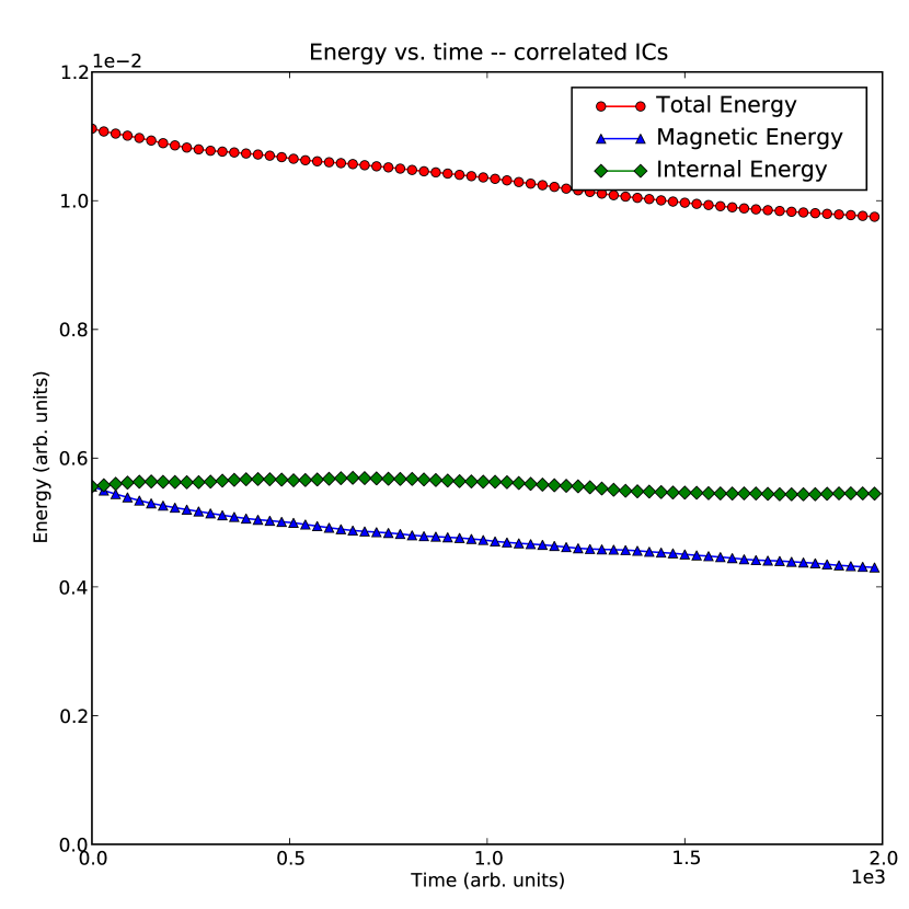
Figure 1: Energy vs. time for cross-correlated initial conditions. Total energy is monotonically decreasing with time, and magnetic and internal energies remain in rough equipartition.

Figure 3: Contours of $n$ for various times in a numerical solution with correlated initial conditions.

Figure 13: Magnitude of magnetic field contour visualization with diffusive damping parameter $\mu=0$ for various times.

References

- Bale et al. (2005) Bale, S.D., Kellogg, P.J., Mozer, F.S., Horbury, T.S. & Reme, H. 2005, Phys. Rev. Lett., 94, 215002
- Biskamp & Welter (1989) Biskamp, D. & Welter, H. 1989, Phys. Fluids B, 1, 1964
- Boldyrev & Gwinn (2003a) Boldyrev, S. & Gwinn, C.R. 2003a, ApJ, 584, 791
- Boldyrev & Gwinn (2003b) Boldyrev, S. & Gwinn, C.R. 2003b, Phys. Rev. Lett., 91, 131101
- Boldyrev & Gwinn (2005) Boldyrev, S. & Gwinn, C.R. 2005, ApJ, 624, 213
- Boldyrev & Konigl (2006) Boldyrev, S. & Konigl, A. 2006, ApJ, 640, 344
- Canuto et al. (1990) Canuto, C., Hussaini, M., Quarteroni, A., & Zang, T. 1990, Spectral Methods in Fluid Dynamics (Berlin:Springer)
- Craddock et al. (1991) Craddock, G.G., Diamond, P.H., & Terry, P.W. 1991, Phys. Fluids B, 3, 304
- Fernandez & Terry (1997) Fernandez, E. & Terry, P.W. 1997, Phys. Plasmas, 4, 2443
- Ferrière (2001) Ferrière, K.M. 2001, Rev. Mod. Phys., 73, 1031
- Goldreich & Sridhar (1995) Goldreich, P. & Sridhar, S. 1995, ApJ, 438, 763
- Harmon & Coles (2005) Harmon, J.K. & Coles, W.A. 2005, J. Geophys. Res., 110, A03101
- Hazeltine (1993) Hazeltine, R.D. 1983, Phys. Fluids, 26, 3242
- Hollweg (1999) Hollweg, J.V. 1999, J. Geophys. Res., 104, 14811
- Howes et al. (2006) Howes, G.G., Cowley, S.C., Dorland, W., Hammett, G.W., Quataert, E. & Schekochihin, A.A. 2006, ApJ651, 590
- Kinney & McWilliams (1995) Kinney, R. & McWilliams, J.C. 1995 The Role of Coherent Structures in Magnetohydrodynamic Turbulence in Proceedings of Small-Scale Structures in Three-Dimensional Hydrodynamic and Magnetohydrodynamic Turbulence, Nice, France, eds. Meneguzzi, M., Pouquet, A. & Sulem, P.L. Lecture Notes in Physics, LNP-462 (Berlin:Springer)
- Lee & Jokipii (1975a) Lee, L.C. & Jokipii, J.R. 1975a, ApJ, 196, 695
- Lee & Jokipii (1975b) Lee, L.C. & Jokipii, J.R. 1975b, ApJ, 201, 532
- Leamon et al. (1998) Leamon, R.J., Smith, C.W., Ness, N.F., Matthaeus, W.H., & Wong, H.K. 1998, J. Geophys. Res., 103, 4775
- Lysak & Lotko (1996) Lysak, R.L. & Lotko, W. 1996, J. Geophys. Res., 101, 5085
- McWilliams (1984) McWilliams, J. 1984, J. Fluid Mech., 146, 21
- Orszag (1971) Orszag, S.A. 1971, J. Atmos. Sci., 28, 1074
- Politano et al. (1989) Politano, H., Pouquet, A., & Sulem, P.L. 1989, Phys. Fluids B, 1, 2330
- Rahman & Wieland (1983) Rahman, H.O. & Weiland, J. 1983, Phys. Rev. A, 28, 1673
- She & Leveque (1994) She, Z.S. & Leveque, E. 1994, Phys. Rev. Lett., 72, 336
- Sutton (1971) Sutton, J.M. 1971, MNRAS, 155, 51
- Terry et al. (2001) Terry, P.W., McKay, C., & Fernandez, E. 2001, Phys. Plasmas, 8, 2707
- Terry & Smith (2007) Terry, P.W., Smith, K.W. 2007, ApJ, 665, 402
- Terry & Smith (2008) Terry, P.W., Smith, K.W. 2008, Phys. Plasmas, 15, 056502
- Williamson (1972) Williamson, I.P. 1972, MNRAS, 157, 55
- Williamson (1973) Williamson, I.P. 1973, MNRAS, 163, 345
- Williamson (1974) Williamson, I.P. 1974, MNRAS, 166, 499