PT-Symmetric Oligomers: Analytical Solutions, Linear Stability and Nonlinear Dynamics

Abstract

In the present work we focus on the case of (few-site) configurations respecting the PT-symmetry. We examine the case of such “oligomers” with not only 2-sites, as in earlier works, but also the cases of 3- and 4-sites. While in the former case of recent experimental interest, the picture of existing stationary solutions and their stability is fairly straightforward, the latter cases reveal a considerable additional complexity of solutions, including ones that exist past the linear PT-breaking point in the case of the trimer, and more complex, even asymmetric solutions in the case of the quadrimer with nontrivial spectral and dynamical properties. Both the linear stability and the nonlinear dynamical properties of the obtained solutions are discussed.

I Introduction

Over the past decade, the examination of Hamiltonian nonlinear dynamical lattices, as well as that of continuum systems with periodic potentials has been a subject of intense investigation reviews . The motivation for such studies stems from a variety of physical settings including, among others, the themes of optical beam dynamics in coupled waveguide arrays or optically induced photonic lattices in photorefractive crystals reviews1 , the temporal evolution of Bose-Einstein condensates (BECs) in optical lattices reviews2 , or the DNA double strand denaturation in biophysics reviews3 . One of the common focal points among all of these areas has been the intense study of the existence, stability and dynamical properties of their nonlinear (often localized in the form of solitary waves) solutions which are of principal interest and experimental observability within various applications; see pgk_rev for a relevant recent review.

On the other hand, as the understanding of the conservative aspects of such systems comes to a point of maturation, a number of interesting variants thereof arise. A canonical one concerns the examination of effects of damping and driving that not only yield novel theoretical solutions (see as an example maniadis ), but also are inherently relevant to applications (again, see for a recent example lars ). A more exotic variant which, however, in the past couple of years has gained considerable momentum especially due to the recent experiments of kip is that of PT-symmetric dynamical lattices. This theme follows the pioneering realization of Bender and coworkers bend that non-Hermitian Hamiltonians can still yield real spectra, provided that they respect the Parity (P) and Time-reversal (T) symmetries. Practically, in the presence of a (generally complex) potential the relevant transformations imply that the potential satisfies the condition $V(x)=V^{\star}(-x)$. In nonlinear optics, the interest in such applications was initiated by the key contributions of Christodoulides and co-workers christo1 which considered solitary waves as well as linear (Floquet-Bloch) eigenmodes in periodic potentials satisfying the above condition, also including the effects of Kerr nonlinearity and observing how the properties of such waves were modified by genuinely complex, yet PT-symmetric potentials.

More recently, motivated by the experimental possibilities and the relevant realization of a PT-“coupler” in kip , there has been an interest in merging the experience of the above two areas, namely the consideration of PT-symmetric settings but for genuinely discrete media. In that vein, the experimentally-probed two-site system has been considered in the work of kot1 , where it was shown that it can operate as a unidirectional optical valve, as well as in the study of sukh1 , where the role of nonlinearity in allowing (if sufficiently weak) or suppressing (if sufficiently strong) time reversals of exchanges of optical power between the sites. Another recent example consisted of the generalization of kot2 where a lattice of coupled gain-loss dimers was considered. This theme has also been considered in the BEC literature and in the context of the so-called leaky Bose-Hubbard dimers (allowing e.g. the tunneling escape of atoms from one of the wells of a double-well potential). There, a variant of the model considered below has been self-consistently derived in the mean-field approximation grae1 and the correspondence of its classical with the full quantum behavior has been explored grae2 .

Our aim in the present work is to revisit the examination of the PT-symmetric coupler and to give a simple and complete characterization of the existence and stability properties of its stationary solutions. It should be noted that this aspect has been partly addressed in both kot1 and sukh1 . Nevertheless, we aim to give a characterization thereof as a preamble towards the more complex (and thus, arguably, more interesting) generalization to what we call “PT-symmetric oligomers”, namely the consideration of a PT-symmetric trimer and that of a PT-symmetric quadrimer. Our aim here is to explore how the complexity of the problem expands as more sites are added, in order to offer a glimpse how such oligomers gradually give way to the elaborate phenomenology of a PT-symmetric lattice. We illustrate, for example, how it is possible in the case of a trimer to identify stationary solutions which exist past the limit of linear PT-symmetry breaking (something which is not possible in the dimer case). We then proceed to illustrate how the phenomenology of the quadrimer is even richer and more complex, featuring among others asymmetric solutions with a reduced symmetry spectrum differently than is the case for both the dimer and trimer.

Our presentation will be structured as follows. In section II, we consider the fundamental (and previously considered) dimer case. We use this as a benchmark for the presentation of our methods and results. We then turn to the more complex trimer case in section III and conclude our results with section IV on the quadrimer. Finally, section V summarizes our findings and presents some interesting questions for further study.

II Dimer

We start our considerations from the so-called PT-symmetric coupler or dimer (as we will call it hereafter). In this case, the dynamical equations are of the form:

$$i\dot{u}_{1} = -ku_{2}-|u_{1}|^{2}u_{1}-i\gamma u_{1}$$

$$i\dot{u}_{2} = -ku_{1}-|u_{2}|^{2}u_{2}+i\gamma u_{2}.$$ (1)

The model of Eq. (1) considers the linear PT-symmetric dimer experimentally examined in kip , as augmented by the Kerr nonlinearity relevant e.g. to optical waveguides; see also kot1 ; sukh1 . The overdot denotes the derivative with respect to the evolution variable which in optical applications is the propagation distance. In what follows, we will denote this variable by $t$ (to indicate its evolutionary nature). We seek stationary solutions of the form $u_{1}=\exp(iEt)a$ and $u_{2}=\exp(iEt)b$. Then the stationary equations arise:

$$Ea = kb+|a|^{2}a+i\gamma a$$

$$Eb = ka+|b|^{2}b-i\gamma b.$$ (2)

Using a generic polar representation of the two “sites” $a=Ae^{i\phi_{a}},b=Be^{i\phi_{b}}$, we are led to the following algebraic conditions for the two existing branches of solutions (notice the $\pm$ sign distinguishing between them):

$$A^{2}=B^{2}=E\pm\sqrt{k^{2}-\gamma^{2}}$$ (3)

$$\sin(\phi_{b}-\phi_{a})=-\frac{\gamma}{k}$$ (4)

The fundamental difference of such solutions from their standard Hamiltonian ($\gamma=0$) counterpart is that the latter were lacking the “flux condition” of Eq. (4). This dictated a selection of the phases so that no phase current would arise between the sites. On the contrary, in PT-symmetric settings, the phase flux is nontrivial and must, in fact, be consonant with the gain-loss pattern of the coupler.

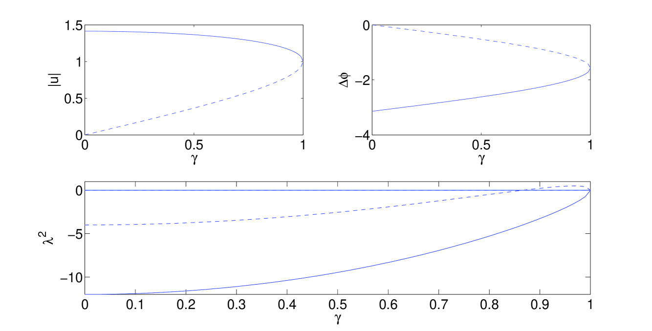
Figure 1: The two branches of solutions for the dimer problem are shown for parameter values $k=E=1$. The top left illustrates the amplitude of the sites, the top right their relative phase and the bottom panel shows the (nontrivial) squared eigenvalue of the two branches. The solid line corresponds to the always stable branch $u^{(2)}$, while the dashed branch corresponds to $u^{(1)}$, which acquires a real eigenvalue pair above a certain $\gamma=\sqrt{k^{2}-E^{2}/4}$.

Fig. 1 shows the profile of the two branches. The first branch $u^{(1)}$ corresponding to the $(-)$ sign in Eq. (3) is stable when $\gamma^{2}\leq k^{2}-E^{2}/4$, whereas the second branch $u^{(2)}$ is always stable. The linearization around these branches can be performed explicitly yielding the nonzero eigenvalue pairs $\pm 2i\sqrt{2(k^{2}-\gamma^{2})-E\sqrt{k^{2}-\gamma^{2}}}$ for the first and $\pm 2i\sqrt{2(k^{2}-\gamma^{2})+E\sqrt{k^{2}-\gamma^{2}}}$ for the second (notice that the latter can never become real).

It is relevant to note here that the two branches “die” in a saddle-center bifurcation at $\gamma=k$, as shown in the figure. Importantly, this coincides with the linear limit of the PT-symmetry breaking since the linear eigenvalues of the problem are $\lambda=\pm\sqrt{k^{2}-\gamma^{2}}$. Hence, the nonlinear solutions terminate where the linear problem eigenfunctions yield an imaginary pair, predisposing us for an asymmetric evolution past this critical point (for all initial data). The dynamical evolution of the dimer is shown first for a case of $\gamma<k$ (in which $u^{(1)}$ is unstable, while $u^{(2)}$ is stable) in Fig. 2. The evolution of the instability of $u^{(1)}$ leads to an asymmetric distribution of the power in the coupler, despite the fact that parametrically we are below the linear critical point (for the PT-symmetry breaking). Notice that in all the cases, also below, where a stationary solution exists for the parameter values for which it is initialized, dynamical instabilities arise only through the amplification of roundoff errors i.e., a numerically exact solution up to $10^{-8}$ is typically used as an initial condition in the system. Naturally, beyond $\gamma=k$, as shown in Fig. 3, all initial data yield such an asymmetric evolution.

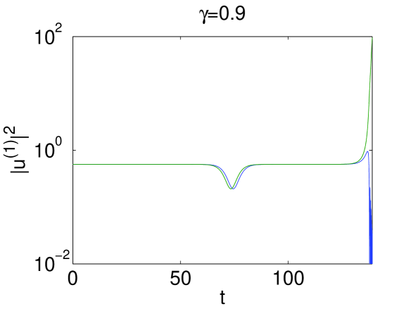
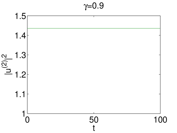
Figure 2: Dynamical evolution of initial data belonging to the two branches of stationary solutions of a dimer in the case of $\gamma=0.9,\ E=k=1$, which is past the critical point for the instability of the first branch (left panel), while the second branch of the right panel is still dynamically stable. Notice that the left panel is plotted in semilog.

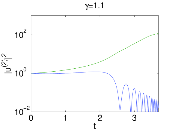
Figure 3: Similar initialization of the dimer based on the two branches of stationary solutions (for $\gamma=1$) but now for the case of $\gamma=1.1$ ($E=k=1$). The asymmetric evolution of the coupler past the linear PT-symmetric threshold can be clearly discerned.

III Trimer

We now turn to the case of the trimer where the dynamical equations are

$$i\dot{u}_{1} = -ku_{2}-|u_{1}|^{2}u_{1}-i\gamma u_{1}$$

$$i\dot{u}_{2} = -k(u_{1}+u_{3})-|u_{2}|^{2}u_{2}$$

$$i\dot{u}_{3} = -ku_{2}-|u_{3}|^{2}u_{3}+i\gamma u_{3}$$ (5)

Seeking once again stationary solutions leads to the algebraic equations

$$Ea = kb+|a|^{2}a+i\gamma a$$

$$Eb = k(a+c)+|b|^{2}b$$

$$Ec = kb+|c|^{2}c-i\gamma c$$ (6)

In this case too, it is helpful to use the polar representation for the three-sites in the form $a=Ae^{i\phi_{a}},b=Be^{i\phi_{b}},c=Ce^{i\phi_{c}}$, which, in turn, leads to the algebraic equations of the form:

$$A=C$$ (7)

$$B^{4}-EB^{2}+2EA^{2}-2A^{4}=0$$ (8)

$$\sin(\phi_{b}-\phi_{a})=-\sin(\phi_{b}-\phi_{c})=-\frac{\gamma A}{kB}$$ (9)

$$\cos(\phi_{a}-\phi_{b})=\cos(\phi_{b}-\phi_{c})=\frac{EA-A^{3}}{kB}$$ (10)

Notice how the presence of the gain-loss spatial profile along the 3-sites induces a spatial phase distribution and enforces the condition of a symmetric amplitude profile with the first and third site sharing the same amplitude. This phase distribution would be trivial (relative phases of $0$ or $\pi$) in the $\gamma=0$ case.

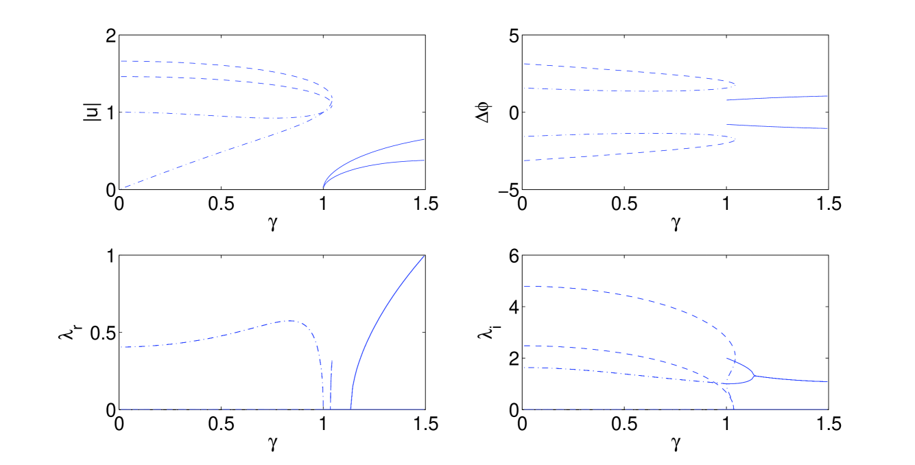
Figure 4: Existence and stability of solutions for the case of the trimer analogously to Fig. 1 for the dimer case. The only other difference is the illustration of both real and imaginary parts for the eigenvalues in the bottom panel. We have set (without loss of generality) $\phi_{b}$ normalized to $0$. Different line styles are used to distinguish different branches and their corresponding stabilities (see the detailed explanation in the text).

A typical example of the branches that may arise in the case of the trimer is shown in Fig. 4 for $E=k=1$. In this case, we find three distinct branches in the considered interval of parameter values. There are two branches which exist up to the critical point $\gamma=1.043$. In this interval one of the two branches $u^{(1)}$ is chiefly unstable (denoted by dash-dotted line) except for a small interval of $\gamma\in[1,1.035]$. The other one $u^{(2)}$ is chiefly stable (denoted by a dashed line) except for $\gamma\in[1.035,1.043]$. The eigenvalues of $u^{(1)}$ and $u^{(2)}$ in $\gamma\in[1.035,1.043]$ are very close to each other but not identical. Notice that $u^{(1)}$ is unstable due to a complex eigenvalue quartet whose eigenvalues collide on the imaginary axis for $\gamma=1$ and split into two imaginary pairs one of which becomes real for $\gamma>1.035$. Finally, these two branches collide in a saddle-center bifurcation (for $\gamma=1.043$) and disappear thereafter.

Interestingly, however, these are not the only branches that arise in the trimer case. In particular, as can be seen in Fig. 4, there is a branch of solutions bifurcating from zero (amplitude) for $\gamma>\sqrt{2k^{2}-E^{2}}$, denoted by $u^{(3)}$, the solid line in Fig. 4. In our case $E=k=1$, this branch is only stable for $\gamma<1.13$, at which point two pairs of imaginary eigenvalues collide and lead to a complex quartet which renders the branch unstable thereafter. Yet, this branch of solutions has a remarkable trait. In the case of the trimer, the underlying linear problem possesses the following eigenvalues $0$, $\pm\sqrt{2k^{2}-\gamma^{2}}$. Hence, the critical point for the existence of real eigenvalues of the linear problem in the case of the PT-symmetric trimer is $\gamma=\sqrt{2}k$ (cf. with the $\gamma=k$ limit of the dimer). Nevertheless, and contrary to what is the case for the dimer, the third branch of solutions considered above persists beyond this critical point (although it is unstable in that regime).

The evolution of the three distinct branches of solutions, namely the chiefly unstable one $u^{(1)}$, the chiefly stable one $u^{(2)}$ and finally of the one persisting past the linearly unstable limit $u^{(3)}$ is shown, respectively, in Figs. 5, 6 and 7. It can be seen that in accordance with the predictions of our linear stability analysis the first two branches are stable or unstable in their corresponding regimes, while past the point of existence of these branches ($\gamma=1.043$) their evolution gives rise to asymmetric dynamics favoring the growth of the power in a single site (or in some cases even in two sites; see e.g. the bottom panels of Figs. 5 and 6). On the other hand, for the branch emerging at $\gamma=1$ and persisting past the linear instability limit, we indeed find it to be stable for $\gamma<1.13$ and unstable thereafter again leading to an asymmetric distribution of the power.

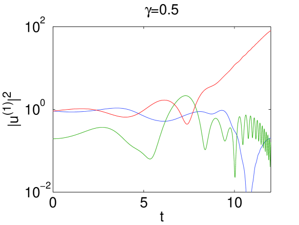
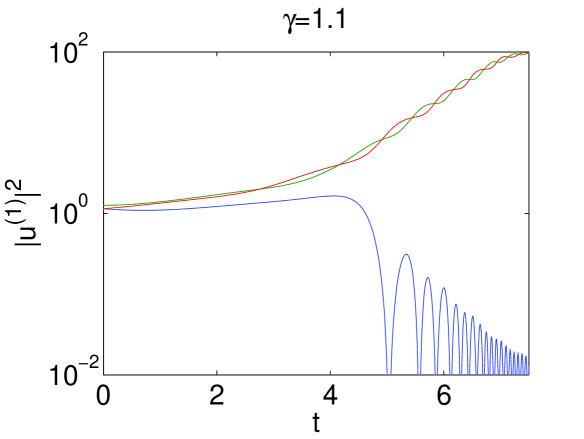
Figure 5: The dynamical evolution of the amplitudes of the three sites of the stationary solution $u^{(1)}$ in the case of $E=k=1$ for $\gamma=0.5$ (left panel), $\gamma=1.03$ (right panel) and $\gamma=1.1$ (bottom panel). The bottom panel is initialized with the exact stationary solution for $\gamma=1.04$ (since for $\gamma=1.1$ the branch no longer exists as a stationary solution).

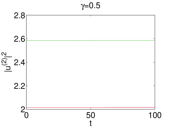
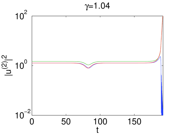
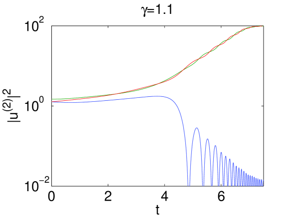
Figure 6: Similar to Fig. 5 but for the case of $u^{(2)}$ and for $E=k=1$. The bottom panel is again initialized for $\gamma=1.04$.

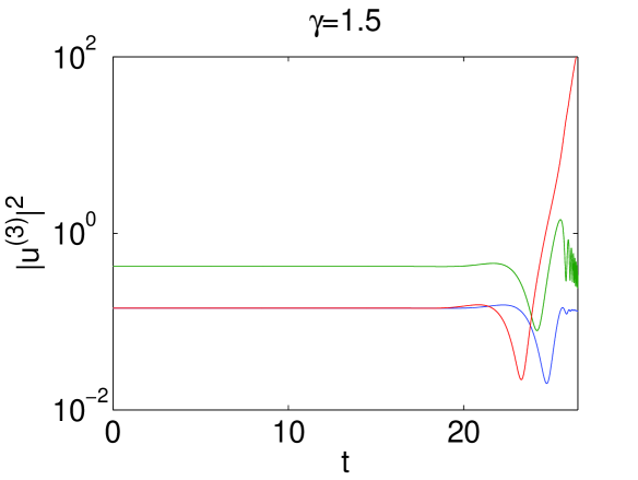
Figure 7: The dynamical evolution for the case of $u^{(3)}$ and for $E=k=1$; $\gamma=1.04$ is used in the left panel and $\gamma=1.5$ in the right one.

IV Quadrimer

Finally, we briefly turn to the case of the quadrimer. Here the equations are:

$$i\dot{u}_{1} = -ku_{2}-|u_{1}|^{2}u_{1}-i\gamma u_{1}$$

$$i\dot{u}_{2} = -k(u_{1}+u_{3})-|u_{2}|^{2}u_{2}-i\gamma u_{2}$$

$$i\dot{u}_{3} = -k(u_{2}+u_{4})-|u_{3}|^{2}u_{3}+i\gamma u_{3}$$

$$i\dot{u}_{4} = -ku_{3}-|u_{4}|^{2}u_{4}+i\gamma u_{4}$$ (11)

Notice here that we only consider the case where the first two sites have the same loss and the latter two the same gain. This is by no means necessary and the gain-loss profile can be generalized to involve two-parameters (e.g. $\pm\gamma_{1}$ and $\pm\gamma_{2}$ distinct between the different corresponding sites i.e., the first and fourth ones, as well as the second and third ones). We do not consider this latter case here, due to its more complicated algebraic structure that does not permit the direct analytical results given below. More specifically, in our considered special case, the stationary equations read:

$$Ea = kb+|a|^{2}a+i\gamma a$$

$$Eb = k(a+c)+|b|^{2}b+i\gamma b$$

$$Ec = k(b+d)+|c|^{2}c-i\gamma c$$

$$Ed = kc+|d|^{2}d-i\gamma d$$ (12)

The polar representation of the form $a=Ae^{i\phi_{a}},b=Be^{i\phi_{b}},c=Ce^{i\phi_{c}},d=De^{i\phi_{d}}$ now allows the following reduced algebraic equations:

$$A^{2}+B^{2}=C^{2}+D^{2}=E$$ (13)

$$A^{2}B^{4}+\gamma^{2}A^{2}-k^{2}B^{2}=0$$ (14)

$$D^{2}C^{4}+\gamma^{2}D^{2}-k^{2}C^{2}=0$$ (15)

$$\sin(\phi_{b}-\phi_{a})=-\frac{\gamma A}{kB}$$ (16)

$$\sin(\phi_{c}-\phi_{b})=-\frac{\gamma E}{kBC}=-1$$ (17)

$$\sin(\phi_{d}-\phi_{c})=-\frac{\gamma D}{kC}.$$ (18)

Notice that in this case not only do we have the customary phase profile, but in fact one of the phase differences becomes locked to $\pi/2$ due to the presence of the gain-loss pattern.

Upon reducing the algebraic equations, we obtain

$$(E-B^{2})B^{4}+\gamma^{2}(E-B^{2})-k^{2}B^{2}=0$$ (19)

$$(E-C^{2})C^{4}+\gamma^{2}(E-C^{2})-k^{2}C^{2}=0$$ (20)

$$\gamma E=kBC$$ (21)

This leads to the important conclusion that for this gain-loss profile in the case of the quadrimer, differently than in the cases of the dimer and trimer, one of the parameters $E,\ k,\ \gamma$ is determined by the other two; i.e., not all three of these parameters can be picked independently in order to give rise to a solution of the quadrimer.

We hereby set $E=1$, and increase $\gamma$ from $0$ as before, then $k$ can be obtained self-consistently from the above equations. Therefore, once $E$ and $\gamma$ are fixed, the solutions of the quadrimer problem are fully determined. We now present three branches of solutions that arise in this setting, as we increase $\gamma$. These are shown in the panels of Fig. 8. There are two classes of solutions here. The solid curve $u^{(1)}$ corresponds to a fully asymmetric branch with $A$, $B$, $C$, $D$ distinct, something that is unique (among the settings considered herein) to the quadrimer. Furthermore, this always unstable branch does not respect the Hamiltonian eigenalue symmetry i.e., that if $\lambda$ is an eigenvalue, so are $-\lambda$, $\lambda^{\star}$ and $-\lambda^{\star}$. On the other hand, the dashed curve of the branch $u^{(2)}$ and the dash-dotted curve of $u^{(3)}$ correspond to symmetric branches with amplitudes $A=D$ and $B=C$. Among the two symmetric branches $u^{(2)}$ and $u^{(3)}$ that collide and disappear together in a saddle-center bifurcation at $\gamma=0.362$, we can observe that the former one between them has a real and two imaginary pairs of eigenvalues being always unstable, while the latter starts out stable, but the collision of two of its imaginary pairs will render it unstable past the critical point of $\gamma=0.023$. Interestingly the asymmetric branch $u^{(1)}$ and the symmetric branch $u^{(3)}$ appear to collide in a subcritical pitchfork bifurcation that imparts the instability of the asymmetric branch to the symmetric one for $\gamma>0.193$.

As an aside, we should also note here that in its linear dynamics (examined e.g. experimentally in kip ) the PT-symmetric quadrimer has an interesting difference from the dimer and trimer. In particular, the 4 linear eigenvalues of the system are:

$$\lambda_{1,2}=\pm\sqrt{-\gamma^{2}+\frac{k}{2}\left(3k-\sqrt{-16\gamma^{2}+5k^{2}}\right)}$$ (22)

$$\lambda_{3,4}=\pm\sqrt{-\gamma^{2}+\frac{k}{2}\left(3k+\sqrt{-16\gamma^{2}+5k^{2}}\right)}.$$ (23)

The fundamental difference of this case from the others considered above is that these eigenvalues do not become imaginary by crossing through 0. Instead, they become genuinely complex, through their collision which occurs for $\gamma=\sqrt{5}k/4$, a critical point which is lower than that of the trimer. This could be an experimentally observable signature of the difference between the near linear dynamics of the quadrimer in comparison e.g. to the trimer.

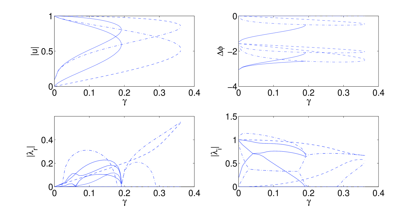
Figure 8: Three branches of solutions for the trimer problem with parameters $E=1$ and $\phi_{a}$ normalized to $0$: the solid lines denote the asymmetric branch $u^{(1)}$, while the dashed and dash-dotted denote the symmetric branches $u^{(2)}$ and $u^{(3)}$, respectively.

The dynamics of these different branches was also considered in Fig. 9. In this case, it can be clearly observed that all three branches tend towards an asymmetric distribution of the power. This favors the two sites (third and fourth) with the gain, although some case examples can be found (see e.g. the top left panel of Fig. 9 for the asymmetric branch), where only one of the two gain sites is favored by the mass evolution.

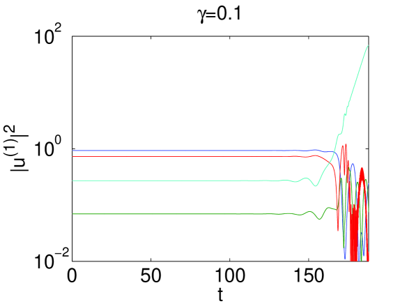
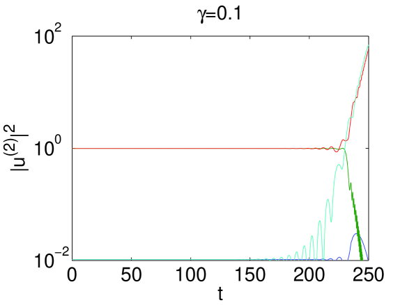
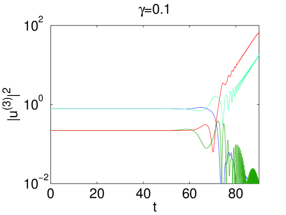
Figure 9: The profile of the dynamical evolution of the three different branches (top left for $u^{(1)}$, top right for $u^{(1)}$ and bottom panel for $u^{(3)}$) of a quadrimer in the case of $E=1$ and $\gamma=0.1$.

V Conclusions

In the present work, we considered the existence, stability and dynamics of PT-symmetric oligomers i.e., configurations with few sites. Similarly to the recent works of kot1 ; sukh1 and also the experimental investigation of kip , we have started our considerations by a complete characterization of the dimer case, where the two obtained branches of solutions terminate at the critical point of the linear case. However, we illustrated that the trimer and quadrimer feature a number of fundamental differences in comparison with this dimer behavior. In particular, the trimer features branches which exist past the linear critical point (although unstable). On the other hand, the quadrimer has even richer features: in particular, it possesses asymmetric solutions whose spectrum only has symmetry around the x-axis (and not the four-fold symmetry of the $\gamma=0$ Hamiltonian problem). The bifurcation structure is also richer in the latter problem featuring symmetry-breaking pitchfork bifurcations. Another notable feature is that solutions do not exist for arbitrary combinations of coupling, gain/loss parameter and propagation constant; instead, these parameters appear to be inter-connected (at least in the case of a single gain-loss parameter considered herein). Finally, even the linear problem presents interesting variations in this case, featuring the breaking of the real nature of the eigenvalues through two colliding pairs that lead to a quartet occuring for smaller gain/loss parameter values than in the trimer case.

This investigation may be a first step towards obtaining a deeper analytical understanding of the features of PT-symmetric lattices. In such settings it would be relevant to obtain general conclusions both for the linear dynamics (and how it depends on the gain/loss profile parameters) as well as more importantly for the nonlinear modes, including the solitary waves that may arise. Understanding such modes and the comparison of their properties to the continuum ones, as well as to the discrete ones in the absence of the gain/loss would be important directions for future study.

- (1) S. Aubry, Physica D 103, 201, (1997); S. Flach and C.R. Willis, Phys. Rep. 295 181 (1998); D. Hennig and G. Tsironis, Phys. Rep. 307, 333 (1999); P.G. Kevrekidis, K.O. Rasmussen, and A.R. Bishop, Int. J. Mod. Phys. B 15, 2833 (2001). A. Gorbach and S. Flach, Phys. Rep. 467, 1 (2008).
- (2) D. N. Christodoulides, F. Lederer and Y. Silberberg, Nature 424, 817 (2003); Yu. S. Kivshar and G. P. Agrawal, Optical Solitons: From Fibers to Photonic Crystals, Academic Press (San Diego, 2003).
- (3) P.G. Kevrekidis and D.J. Frantzeskakis, Mod. Phys. Lett. B 18, 173 (2004). V.V. Konotop and V.A. Brazhnyi, Mod. Phys. Lett. B 18 627, (2004); O. Morsch and M. Oberthaler, Rev. Mod. Phys. 78, 179 (2006).
- (4) M. Peyrard, Nonlinearity 17, R1 (2004).
- (5) P.G. Kevrekidis, arXiv:1009.3178 (IMA J. Appl. Math., in press).
- (6) P. Maniadis and S. Flach, Europhys. Lett. 74, 452 (2006).
- (7) J. Cuevas, L.Q. English, P.G. Kevrekidis and M. Anderson, Phys. Rev. Lett. 102, 224101 (2009).
- (8) C.E. Rüter, K.G. Makris, R. El-Ganainy, D.N. Christodoulides, M. Segev, D. Kip, Nature Phys. 6, 192 (2010).
- (9) C.M. Bender and S. Boettcher, Phys. Rev. Lett. 80, 5243 (1998); C.M. Bender, S. Boettcher and P.N. Meisinger, J. Math. Phys. 40, 2201 (1999); C.M. Bender, Rep. Prog. Phys. 70, 947 (2007).
- (10) Z.H. Musslimani, K.G. Makris, R. El-Ganainy and D.N. Christodoulides, Phys. Rev. Lett. 100, 030402 (2008); K.G. Makris, R. El-Ganainy, D.N. Christodoulides and Z.H. Musslimani, Phys. Rev. A 81, 063807 (2010).
- (11) H. Ramezani, T. Kottos, R. El-Ganainy and D.N. Christodoulides, Phys. Rev. A 82, 043803 (2010).
- (12) A.A. Sukhorukov, Z. Xu and Yu.S. Kivshar, Phys. Rev. A 82, 043818 (2010).
- (13) M.C. Zheng, D.N. Christodoulides, R. Fleischmann and T. Kottos, Phys. Rev. A 82, 010103(R) (2010).
- (14) E.M. Graefe, H.J. Korsch and A.E. Niederle, Phys. Rev. Lett. 101, 150408 (2008).
- (15) E.M. Graefe, H.J. Korsch and A.E. Niederle, Phys. Rev. A 82, 013629 (2010).