Temperature dependent resistivity in bilayer graphene due to flexural phonons

Abstract

We have studied electron scattering by out-of-plane (flexural) phonons in doped suspended bilayer graphene. We have found the bilayer membrane to follow the qualitative behavior of the monolayer cousin. In the bilayer, different electronic structure combine with different electron-phonon coupling to give the same parametric dependence in resistivity, and in particular the same temperature $T$ behavior. In parallel with the single layer, flexural phonons dominate the phonon contribution to resistivity in the absence of strain, where a density independent mobility is obtained. This contribution is strongly suppressed by tension, and in-plane phonons become the dominant contribution in strained samples. Among the quantitative differences an important one has been identified: room $T$ mobility in bilayer graphene is substantially higher than in monolayer. The origin of quantitative differences has been unveiled.

I Introduction

Bilayer graphene continues to attract a great deal of attention because of both fascinating fundamental physicsFeldman et al. (2009) and possible applications.Zhang et al. (2009) Recent realization of suspended monolayerBolotin et al. (2008); Du et al. (2008) and bilayerFeldman et al. (2009) graphene samples made possible a direct probe of the intrinsic, unusual properties of these systems. In particular, intrinsic scattering mechanisms limiting mobility may now be unveiled.Morozov et al. (2008) It has been recently shown that in suspended, non-strained monolayer graphene room temperature $T$ mobility is limited to values observed for samples on substrate due to scattering by out of plane — flexural — acoustic phonons.Castro et al. (2010) This limitation can, however, be avoided by applying tension. Bilayer graphene has a different low energy electronic behavior as well as different electron-phonon coupling. It is then natural to wonder what is the situation in the bilayer regarding electron scattering by acoustic phonons, and in particular by flexural phonons (FPs).

In the present work the $T$ dependent resistivity due to scattering by both acoustic in-plane phonons and FPs in doped, suspended bilayer graphene, has been investigated. We have found the bilayer membrane to follow the qualitative behavior of the monolayer parent.Mariani and von Oppen (2010); Castro et al. (2010) Explicitly, at experimentally relevant $T$, the non-strained samples show quadratic in $T$ resistivity with logarithmic correction, $\varrho\sim T^{2}\ln(T)$, and constant mobility. Electron scattering by two FPs gives the main contribution to the resistivity in this case, and is responsible for the $T^{2}$ dependence. Suspended samples may also be under strain either due to the charging gateOchoa et al. or due to the experimental procedure to get suspended samples, or even by applying strain in a controlled way.Bao et al. (2009); Chen et al. (2009) Under uniaxial or isotropic strain $u$ the $T$ dependence of resistivity due to FPs becomes quartic at high strain $u\gg u^{*}$, $\varrho\sim T^{4}/u^{3}$, and quadratic at low strain $u\ll u^{*}$, $\varrho\sim T^{2}/u$, where $u^{*}\approx 10^{-4}T(\mbox{K})$. These contributions are weaker than that coming from scattering by in-plane phonons, and in strained samples the latter dominates resistivity, as has been found for monolayer graphene.Castro et al. (2010) An interesting quantitative difference with respect to suspended monolayer has been found. In the latter, room $T$ mobility $\mu$ is limited to values obtained for samples on substrate due to FPs, $\mu\sim 1\,\,\mbox{m}^{2}/(\mbox{Vs})$.Castro et al. (2010) In bilayer, quantitative differences in electron-phonon coupling and elastic constants lead to room $T$ enhanced $\mu\sim 10-20\,\,\mbox{m}^{2}/(\mbox{Vs})$, even in non-strained samples.

The paper is organized as follows. In Sec. II we introduce long wavelength acoustic phonons in the framework of elasticity theory. We show how the dispersion relation of FPs are affected by the presence of tension over the sample. Then, we review the electronic low-energy description of bilayer graphene and deduce the electron-phonon coupling within this approach in Sec. III. The variational approach used in order to study the $T$ dependent resistivity due to scattering by in-plane and FPs and a summary of our results in different regimes of $T$ and strain are presented in Sec. IV. Sec. V is devoted to discuss the implications of these results, the differences between monolayer and bilayer and some experimental consequences. Finally, we expose our conclusions in Sec. VI. Some technical aspects are treated in detail in appendices. In Appendix. A we present the collision integral due to scattering by acoustic phonons, and in Appendix B its linearized form is derived. Details on the calculation of the resistivity using the variational method are given in Appendix C. In Appendix D we discuss how anharmonic effects are partially suppressed by the presence of strain.

II Acoustic phonons

At long-wavelengths the elastic behavior of monolayer graphene is well approximated by that of an isotropic continuum membraneCastro Neto et al. (2009); Zakharchenko et al. (2009) whose free-energy reads,(Landau and Lifshitz, 1970; Nelson et al., 2004)

$$\mathcal{F}=\frac{1}{2}\kappa\int dxdy(\nabla^{2}h)^{2}+\frac{1}{2}\int dxdy(\lambda u_{ii}^{2}+2\mu u_{ij}^{2}).$$ (1)

The first and second terms in Eq. (1) represent the bending and stretching energies, respectively. Summation over indices is assumed. In-plane distortions are denoted by $\mathbf{u}(\mathbf{r})$ and out-of-plane $h(\mathbf{r})$, with $\mathbf{r}=(x,y)$, such that the new position is $\vec{X}(\mathbf{r})=(x,y,0)+[u_{x}(\mathbf{r}),u_{y}(\mathbf{r}),h(\mathbf{r})]$. To lowest order in gradients of the deformations the strain tensor appearing in Eq. (1) is

$$u_{ij}=\frac{1}{2}[\partial_{i}u_{j}+\partial_{j}u_{i}+(\partial_{i}h)(\partial_{j}h)],$$ (2)

and owing to the same argument the factor $\sqrt{g}=\sqrt{1+|\nabla h|^{2}}$ in the measure is neglected. The parameter $\kappa$ is the bending rigidity and $\lambda$ and $\mu$ are in-plane elastic constants. Typical parameters for graphene are $\kappa\approx 1\,\mbox{eV}$ and $\mu\simeq 3\lambda\approx 9\,\mbox{eV}\textrm{\AA}^{-2}$,Kudin et al. (2001); Lee et al. (2008); Zakharchenko et al. (2009) with mass density $\rho=7.6\times 10^{-7}\,\mbox{kg/m}^{2}$.

In the case of bilayer graphene, as long as we are not at too high $T$ to excite optical phonons we may, from the elastic point of view, regard bilayer graphene as a thick membrane with mass density and elastic constants twice as high as those for single layer.Zakharchenko et al. (2010a)

The dynamics of the displacement fields is here studied in the harmonic approximation by introducing the Fourier series $\mathbf{u}(\mathbf{r})=\mathcal{V}^{-\frac{1}{2}}\sum_{\mathbf{q}}\mathbf{u}_{\mathbf{q}}e^{i\mathbf{q}.\mathbf{r}}$ and $h(\mathbf{r})=\mathcal{V}^{-\frac{1}{2}}\sum_{\mathbf{q}}h_{\mathbf{q}}e^{i\mathbf{q}.\mathbf{r}}$, where $\mathcal{V}$ is the volume of the system.

II.1 In-plane phonons

The decoupled in-plane phonon modes are obtained in the usual way by changing to longitudinal $u_{\mathbf{q}}^{L}=\mathbf{u}_{\mathbf{q}}\cdot\mathbf{q}/q$ and transverse $u_{\mathbf{q}}^{T}=\mathbf{u}_{\mathbf{q}}\cdot(\hat{e}_{z}\times\mathbf{q}/q)$ displacement fields. The dispersion relations have the usual linear behavior in momentum and are given by

$$\omega_{\mathbf{q}}^{L} = v_{L}q,$$

$$\omega_{\mathbf{q}}^{T} = v_{T}q,$$ (3)

with $v_{L}=\sqrt{\frac{2\mu+\lambda}{\rho}}$ and $v_{T}=\sqrt{\frac{\mu}{\rho}}$. Typical values for monolayer and bilayer graphene are $v_{L}\simeq 2.1\times 10^{4}\,\mbox{m}/\mbox{s}$ and $v_{T}\simeq 1.4\times 10^{4}\,\mbox{m}/\mbox{s}$.

II.2 Flexural phonons

II.2.1 Non-strained case

The quadratic behavior in out-of-plane displacements of the strain tensor in Eq. (2) implies that FP modes are driven by the bending rigidity term. The resulting FP dispersion relation is quadratic,(Mariani and von Oppen, 2008; Castro Neto et al., 2009)

$$\omega_{\mathbf{q}}^{F}=\alpha q^{2},$$ (4)

with $\alpha=\sqrt{\frac{\kappa}{\rho}}$. The typical value is $\alpha\simeq 4.6\times 10^{-7}\,\mbox{m}^{2}/\mbox{s}$.

II.2.2 Strained case

Suspended samples may be under tension either due to the load imposed by the back gate or as a result of the fabrication process, or both. The case of a clamped graphene membrane hanging over a tranche of size $L$, relevant for conventional two-contacts measurements in suspended samples, has been considered in Ref. Fogler et al., 2008.

Once the membrane is under tension a static deformation configuration is expected at equilibrium. The phonon modes may be obtained by assuming that both in-plane $\mathbf{u}(\mathbf{r})$ and flexural $h(\mathbf{r})$ fields have dynamic components which add to their static background: $\mathbf{u}(\mathbf{r})=\mathbf{u}_{st}(\mathbf{r})+\mathbf{u}_{dyn}(\mathbf{r})$ and $h(\mathbf{r})=h_{st}(\mathbf{r})+h_{dyn}(\mathbf{r})$. For the case of the clamped membrane considered in Ref. Fogler et al., 2008 we have $\mathbf{u}_{st}(\mathbf{r})=[u_{x,st}(x),0]$ with $u_{x,st}(x)$ a linear function of $x$, while $h_{st}(x)$ may be approximated by a parabola.

Let us consider the general static displacement vector field $\mathbf{d}_{st}(\mathbf{r})=\left[u_{x,st}(\mathbf{r}),u_{y,st}(\mathbf{r}),h_{st}(\mathbf{r})\right]$ and the associated strain tensor $u_{ij,st}(\mathbf{r})=\frac{1}{2}(\partial_{i}u_{j,st}+\partial_{j}u_{i,st}+\partial_{i}h_{st}\partial_{j}h_{st})$. In-plane phonons are not affected by the static component but the FP dispersion changes considerably. This is a consequence of new harmonic terms appearing due to coupling between in-plane static deformation and out-of-plane vibrations in the full strain tensor in Eq. (2). The resulting FP dispersion relation may be obtained using a local approximation expected to hold for $L\gg\ell=v_{F}\tau\gg k_{F}^{-1}$, where $v_{F}$ is the Fermi velocity, $k_{F}$ the Fermi momentum, and $\tau$ a characteristic collision time. The result reads

$$\omega_{\mathbf{q}}^{F}(\mathbf{r})=q\sqrt{\frac{\kappa}{\rho}q^{2}+u_{ii,st}(\mathbf{r})\frac{\lambda}{\rho}+u_{ij,st}(\mathbf{r})\frac{2\mu}{\rho}\frac{q_{i}q_{j}}{q^{2}}}.$$ (5)

For the particular case of isotropic strain where $u_{xx}=u_{yy}$ and $u_{xy}=0$ the dispersion relation can be cast in the form

$$\omega_{\mathbf{q}}^{F}(\mathbf{r})=q\sqrt{\frac{\kappa}{\rho}q^{2}+u_{ii,st}(\mathbf{r})\frac{\lambda+\mu}{\rho}}.$$ (6)

Here we will give particular emphasis to the clamped membrane case where the FP dispersion is given by

$$\omega_{\mathbf{q}}^{F}=q\sqrt{\frac{\kappa}{\rho}q^{2}+\bar{u}\frac{\lambda+2\mu}{\rho}-\bar{u}\frac{2\mu}{\rho}\sin^{2}\phi_{\mathbf{q}}},$$ (7)

with $\bar{u}\equiv u_{xx}$ and $\phi_{\mathbf{q}}=\arctan(q_{y}/q_{x})$. In order to keep the problem within analytical treatment we will use an effective isotropic dispersion relation, obtained by dropping the angular dependence contribution,

$$\omega_{\mathbf{q}}^{F}\simeq q\sqrt{\alpha^{2}q^{2}+\bar{u}v_{L}^{2}}.$$ (8)

Since we are mainly interested in transport such an approximation has the advantage that backward scattering is still correctly accounted for.

III Electron-phonon interaction

III.1 Low energy description for bilayer graphene

At low energies the 2-band effective model provides a good approximate description for $\pi-$electrons in bilayer graphene.Castro Neto et al. (2009) The $2\times 2$ Hamiltonian can be cast in the form $\mathcal{H}_{eff}=\sum_{\mathbf{k}}\psi_{\mathbf{k}}\mathcal{H}_{\mathbf{k}}\psi_{\mathbf{k}}$, with

$$\mathcal{H}_{\mathbf{k}}=\frac{\hbar^{2}}{2m}\left(\begin{array}[]{cc}0&\left(k_{x}-ik_{y}\right)^{2}\\ \left(k_{x}+ik_{y}\right)^{2}&0\end{array}\right),$$ (9)

where the two component spinor $\psi_{\mathbf{k}}^{\dagger}=[a_{\mathbf{k}}^{\dagger},b_{\mathbf{k}}^{\dagger}]$ stems from the two sublattices not connected by the interlayer hopping, $t_{\perp}\approx 0.3\,\mbox{eV}$. The coupling $t_{\perp}$ between layers sets the effective mass $2m=t_{\perp}/v_{F}^{2}$, with $v_{F}\approx 10^{6}\,\mbox{m}/\mbox{s}$ the Fermi velocity in monolayer graphene. Equation (9) is valid at valley $K$, at valley $K^{\prime}$ we have $\mathcal{H}_{\mathbf{k}}\rightarrow\mathcal{H}_{\mathbf{k}}^{T}$. Here we are interested in electron scattering processes induced by emission or absorption of long wavelength acoustic phonons and hence intervalley scattering is not allowed. Thus we may concentrate on one valley only. The Hamiltonian can be diagonalized introducing the rotated operators

$$d_{\mathbf{k}}=\frac{1}{\sqrt{2}}\left(\begin{array}[]{cc}e^{i\theta_{\mathbf{k}}}&e^{-i\theta_{\mathbf{k}}}\\ e^{i\theta_{\mathbf{k}}}&-e^{-i\theta_{\mathbf{k}}}\end{array}\right)\psi_{\mathbf{k}},$$ (10)

where $\theta_{\mathbf{k}}=\arctan(k_{y}/k_{x})$, with $d_{\mathbf{k}}^{\dagger}=[e_{\mathbf{k}}^{\dagger},h_{\mathbf{k}}^{\dagger}]$ defined such that $e_{\mathbf{k}}^{\dagger}$ stands for electron-like (positive energy) excitations and $h_{\mathbf{k}}^{\dagger}$ for hole-like (negative energy) excitations, from which we get

$$\mathcal{H}=\sum_{\mathbf{k}}\varepsilon\left(\mathbf{k}\right)[e_{\mathbf{k}}^{\dagger}e_{\mathbf{k}}-h_{\mathbf{k}}^{\dagger}h_{\mathbf{k}}],$$ (11)

with $\varepsilon\left(\mathbf{k}\right)=\hbar^{2}k^{2}/(2m)$.

Along the paper we will compare the results obtained for bilayer graphene with those valid in monolayer. The latter is described using the effective Dirac-like Hamiltonian,Castro Neto et al. (2009) which holds in the low energy sector we are interested here.

III.2 Coupling between electrons and phonons

The coupling between electrons and the vibrations of the underlying lattice either in bilayer or monolayer graphene has two main sources. Long wavelength acoustic phonons induce an effective local potential called deformation potential and proportional to the local contraction or dilation of the lattice,(Castro Neto et al., 2009)

$$V_{1}(\mathbf{r})=g_{0}u_{ii}(\mathbf{r}),$$

where $g_{0}$ is the bare deformation potential constant, whose value is in the range $g_{0}\approx 20-30\,\mbox{eV}$.Suzuura and Ando (2002) The respective interaction Hamiltonian is diagonal in sublattice indices and reads

$$\mathcal{H}_{1}=\sum_{\mathbf{k}}\psi_{\mathbf{k}}^{\dagger}\left[V_{1}(\mathbf{k},\mathbf{k}^{\prime})\mathbb{I}\right]\psi_{\mathbf{k}^{\prime}},$$ (12)

where $\mathbb{I}$ is the $2\times 2$ identity matrix and $V_{1}(\mathbf{k},\mathbf{k}^{\prime})$ is the Fourier transform of the deformation potential

$$V_{1}(\mathbf{k},\mathbf{k}^{\prime})=\mathcal{V}^{-1}g_{0}\int d\mathbf{r}e^{i(\mathbf{k}^{\prime}-\mathbf{k})\cdot\mathbf{r}}u_{ii}\left(\mathbf{r}\right).$$ (13)

Equation (12) is valid both for monolayer and bilayer graphene. Since we are interested in doped systems we take into account screening by substituting $V_{1}(\mathbf{k},\mathbf{k}^{\prime})$ with $V_{1}\left(\mathbf{k},\mathbf{k}^{\prime}\right)/\epsilon\left(\mathbf{k}-\mathbf{k}^{\prime}\right)$, where we take a Thomas-Fermi like dielectric function

$$\epsilon\left(\mathbf{q}\right)=1+\frac{e^{2}\mathcal{D}\left(E_{F}\right)}{2\epsilon_{0}q},$$ (14)

and $\mathcal{D}\left(E_{F}\right)$ is the density of states at the Fermi energy, which is given by $\mathcal{D}\left(E_{F}\right)=\frac{2E_{F}}{\pi\hbar^{2}v_{F}^{2}}=\frac{2k_{F}}{\pi\hbar v_{F}}$ in the case of monolayer graphene and by $\mathcal{D}\left(E_{F}\right)=\frac{t_{\perp}}{\pi\hbar^{2}v_{F}^{2}}$ in the case of bilayer.

It is convenient to define $g\equiv g_{0}/\epsilon(k_{F})$ for single layer graphene, which gives a density independent screened deformation potential

$$g\approx\frac{g_{0}}{e^{2}/(\pi\epsilon_{0}\hbar v_{F})}\approx\frac{g_{0}}{8.75}\approx 2-3.5\,\,\mbox{eV}.$$ (15)

Note that the value just obtained is in complete agreement with recent ab initio calculations which give $g\approx 3\,\mbox{eV}$.Choi et al. (2010) It will become clear in Sec. IV.3.1 that $g$ as defined in Eq. (15) is the relevant deformation potential electron-phonon parameter in single layer graphene. For bilayer graphene $g(q)=g_{0}/\epsilon(q)$ gives

$$g(k_{F})\approx\frac{g_{0}}{e^{2}t_{\perp}/(2\pi\epsilon_{0}\hbar^{2}v_{F}^{2}k_{F})}\approx\frac{g_{0}}{11.25}\sqrt{n}\approx(2-3)\sqrt{n}\,\,\mbox{eV},$$ (16)

with $n$ in $10^{12}\,\mbox{cm}^{-2}$. We may then write a $q$ dependent deformation potential electron-phonon parameter which has the form $g_{M}(q)=gq/k_{F}$ for monolayer graphene, and $g_{B}(q)=g2\hbar v_{F}q/t_{\perp}$ for bilayer.

Phonons can also couple to electrons in monolayer and bilayer graphene by changes in bond length and bond angle between carbon atoms. In this case the electron-phonon interaction can be written as due to an effective gauge field,(Morozov et al., 2006; Katsnelson and Novoselov, 2007; Katsnelson and Geim, 2008; Guinea et al., 2008)

$$e\mathbf{A}_{elastic}=\frac{\beta}{a}\Bigl{[}\begin{array}[]{cc}\frac{1}{2}(u_{xx}-u_{yy}),&-u_{xy}\end{array}\Bigr{]},$$

where $\beta\approx-\partial\log t/\partial\log a\sim 2-3$,(Suzuura and Ando, 2002) with $t$ the in-plane nearest neighbor hopping parameter and $a$ the carbon-carbon distance ($t_{0}\approx 3\,\mbox{eV}$ and $a_{0}\approx 1.4\,\textrm{\AA}$). In the case of bilayer graphene the resulting interaction Hamiltonian is obtained by introducing the gauge potential into Eq (9), following the minimal coupling prescription, and keeping only first order terms in electron-phonon coupling. Then we arrive at

$$\mathcal{H}_{2}=\frac{\hbar}{2m}\sum_{\mathbf{k},\mathbf{k}^{\prime}}\psi_{\mathbf{k}}^{\dagger}\left[\begin{array}[]{cc}0&\left(\pi_{\mathbf{k}}^{-}+\pi_{\mathbf{k}^{\prime}}^{-}\right)A_{\mathbf{k},\mathbf{k}^{\prime}}^{-}\\ \left(\pi_{\mathbf{k}}^{+}+\pi_{\mathbf{k}^{\prime}}^{+}\right)A_{\mathbf{k},\mathbf{k}^{\prime}}^{+}&0\end{array}\right]\psi_{\mathbf{k}^{\prime}},$$ (17)

where $\pi_{\mathbf{k}}^{\pm}=ke^{\pm i\theta_{\mathbf{k}}}$, $A_{\mathbf{k},\mathbf{k}^{\prime}}^{\pm}=V_{2,x}(\mathbf{k},\mathbf{k}^{\prime})\pm iV_{2,y}(\mathbf{k},\mathbf{k}^{\prime})$ and the vector $\mathbf{V}_{2}=(V_{2,x},V_{2,y})$ is defined as

$$V_{2,x}(\mathbf{k},\mathbf{k}^{\prime})= \frac{\hbar\beta}{a}\mathcal{V}^{-1}\int d\mathbf{r}e^{i(\mathbf{k}^{\prime}-\mathbf{k})\cdot\mathbf{r}}\frac{1}{2}\left[u_{xx}(\mathbf{r})-u_{yy}(\mathbf{r})\right],$$

$$V_{2,y}(\mathbf{k},\mathbf{k}^{\prime})= -\frac{\hbar\beta}{a}\mathcal{V}^{-1}\int d\mathbf{r}e^{i(\mathbf{k}^{\prime}-\mathbf{k})\cdot\mathbf{r}}u_{xy}(\mathbf{r}).$$ (18)

An estimate of the electron-phonon coupling strength due to $V_{2}$ is given by $k_{F}\hbar^{2}\beta/(ma)\approx(8-12)\sqrt{n}\,\mbox{eV}$, with $n$ in $10^{12}\,\mbox{cm}^{-2}$. In the case of single layer graphene the resulting interaction Hamiltonian reads

$$\mathcal{H}_{2}=v_{F}\sum_{\mathbf{k},\mathbf{k}^{\prime}}\psi_{\mathbf{k}}^{\dagger}\bm{\sigma}\cdot\mathbf{V}_{2}(\mathbf{k},\mathbf{k}^{\prime})\psi_{\mathbf{k}^{\prime}},$$ (19)

where $\bm{\sigma}=(\sigma_{x},\sigma_{y})$ is the vector of Pauli matrices, and the two component spinor $\psi_{\mathbf{k}}^{\dagger}=[a_{\mathbf{k}}^{\dagger},b_{\mathbf{k}}^{\dagger}]$ is reminiscent of the two sublattices of the honeycomb lattice. An estimate of the respective electron-phonon coupling strength is given by $v_{F}\hbar\beta/a\approx 10-15\,\mbox{eV}$.

The electron-phonon interaction Hamiltonian is the sum of the two terms shown above, $H_{ep}=\mathcal{H}_{1}+\mathcal{H}_{2}$. Phonons enter through the strain tensor $u_{ij}$ which we have seen can be written in terms of static and dynamic components; the static ones being zero for zero load. There are purely static terms which do not contribute to electron-phonon scattering and will be dropped (see Ref. Fogler et al., 2008). Quantizing the dynamic part of the displacement fields,(Altland and Simons, 2006) and introducing usual destruction and creation operators $a_{\mathbf{q}}^{\nu}$ and $(a_{\mathbf{q}}^{\nu})^{\dagger}$ for in-plane phonons $\mathbf{q}$ and polarization $\nu=L,T$, we can write the $\mathbf{q}$ component of the in-plane displacement as,

$$u_{\mathbf{q}}^{L/T}=\sqrt{\frac{\hbar}{2\rho\omega_{\mathbf{q}}^{\nu}}}\left[a_{\mathbf{q}}^{L/T}+(a_{-\mathbf{q}}^{L/T})^{\dagger}\right].$$ (20)

For FPs we introduce the bosonic fields $a_{\mathbf{q}}^{F}$ and $(a_{\mathbf{q}}^{F})^{\dagger}$, and write the $\mathbf{q}$ component of the out-of-plane displacement as,

$$h_{\mathbf{q}}=\sqrt{\frac{\hbar}{2\rho\omega_{\mathbf{q}}^{F}}}\left[a_{\mathbf{q}}^{F}+(a_{-\mathbf{q}}^{F})^{\dagger}\right].$$ (21)

The electron-phonon interaction Hamiltonian may then be written either in monolayer or bilayer graphene as,

$$H_{ep}=\sum_{\mathbf{k},\mathbf{k}^{\prime}}\left(a_{\mathbf{k}}^{\dagger}a_{\mathbf{k}^{\prime}}+b_{\mathbf{k}}^{\dagger}b_{\mathbf{k}^{\prime}}\right)\left\{\sum_{\nu,\mathbf{q}}V_{1,\mathbf{q}}^{\nu}\left[a_{\mathbf{q}}^{\nu}+(a_{-\mathbf{q}}^{\nu})^{\dagger}\right]\delta_{\mathbf{k}^{\prime},\mathbf{k}-\mathbf{q}}+\sum_{\mathbf{q},\mathbf{q}^{\prime}}V_{1,\mathbf{q},\mathbf{q}^{\prime}}^{F}\left[a_{\mathbf{q}}^{F}+(a_{-\mathbf{q}}^{F})^{\dagger}\right]\left[a_{\mathbf{q}^{\prime}}^{F}+(a_{-\mathbf{q}^{\prime}}^{F})^{\dagger}\right]\delta_{\mathbf{k}^{\prime},\mathbf{k}-\mathbf{q}-\mathbf{q}^{\prime}}\right\}\\ +\sum_{\mathbf{k},\mathbf{k}^{\prime}}\left\{\sum_{\nu,\mathbf{q}}V_{2,\mathbf{q}}^{\nu}a_{\mathbf{k}}^{\dagger}b_{\mathbf{k}^{\prime}}\left[a_{\mathbf{q}}^{\nu}+(a_{-\mathbf{q}}^{\nu})^{\dagger}\right]\delta_{\mathbf{k}^{\prime},\mathbf{k}-\mathbf{q}}+\sum_{\mathbf{q},\mathbf{q}^{\prime}}V_{2,\mathbf{q},\mathbf{q}^{\prime}}^{F}a_{\mathbf{k}}^{\dagger}b_{\mathbf{k}^{\prime}}\left[a_{\mathbf{q}}^{F}+(a_{-\mathbf{q}}^{F})^{\dagger}\right]\left[a_{\mathbf{q}^{\prime}}^{F}+(a_{-\mathbf{q}^{\prime}}^{F})^{\dagger}\right]\delta_{\mathbf{k}^{\prime},\mathbf{k}-\mathbf{q}-\mathbf{q}^{\prime}}+\mbox{h.c.}\right\}.$$ (22)

For monolayer graphene the matrix elements read,

$$V_{1,\mathbf{q}}^{L} = \frac{g_{0}}{\epsilon(q)}iq\sqrt{\frac{\hbar}{2\mathcal{V}\rho\omega_{\mathbf{q}}^{L}}},$$

$$V_{1,\mathbf{q},\mathbf{q}^{\prime}}^{F} = -\frac{g_{0}}{\epsilon(|\mathbf{q}+\mathbf{q}^{\prime}|)}qq^{\prime}\cos(\phi_{\mathbf{q}}-\phi_{\mathbf{q}^{\prime}})\frac{\hbar}{4\mathcal{V}\rho\sqrt{\omega_{\mathbf{q}}^{F}\omega_{\mathbf{q}^{\prime}}^{F}}},$$

$$V_{1,\mathbf{q}}^{F} = \frac{g_{0}}{\epsilon(q)}iq_{i}\partial_{i}h_{st}\sqrt{\frac{\hbar}{2\mathcal{V}\rho\omega_{\mathbf{q}}^{F}}},$$

$$V_{2,\mathbf{q}}^{L} = \frac{\hbar v_{F}\beta}{2a}iqe^{i2\phi_{\mathbf{q}}}\sqrt{\frac{\hbar}{2\mathcal{V}\rho\omega_{\mathbf{q}}^{L}}},$$

$$V_{2,\mathbf{q}}^{T} = -\frac{\hbar v_{F}\beta}{2a}qe^{i2\phi_{\mathbf{q}}}\sqrt{\frac{\hbar}{2\mathcal{V}\rho\omega_{\mathbf{q}}^{T}}},$$

$$V_{2,\mathbf{q},\mathbf{q}^{\prime}}^{F} = -\frac{\hbar v_{F}\beta}{4a}qq^{\prime}e^{i(\phi_{\mathbf{q}}-\phi_{\mathbf{q}^{\prime}})}\frac{\hbar}{2\mathcal{V}\rho\sqrt{\omega_{\mathbf{q}}^{F}\omega_{\mathbf{q}^{\prime}}^{F}}},$$

$$V_{2,\mathbf{q}}^{F} = \frac{\hbar v_{F}\beta}{2a}iq\left[e^{i\phi_{\mathbf{q}}}\partial_{x}h_{st}+e^{-i\phi_{\mathbf{q}}}\partial_{y}h_{st}\right]\sqrt{\frac{\hbar}{2\mathcal{V}\rho\omega_{\mathbf{q}}^{F}}}\,,$$ (23)

with $V_{1,\mathbf{q}}^{T}=0$ (see also Refs. Mariani and von Oppen, 2008, 2010), and where we have again used the local approximation. In the case of bilayer graphene only the matrix elements for the gauge potential change, becoming dependent on fermionic momenta $\mathbf{k}$ and $\mathbf{k}^{\prime}$. As can be seen by comparing Eqs. (17) and (19), they take exactly the same form as in Eq. (23) with the replacement $v_{F}\rightarrow\hbar(\pi_{\mathbf{k}}+\pi_{\mathbf{k}^{\prime}})/(2m)$.

IV Temperature dependent resistivity

Our aim here is to study the $T$ dependent resistivity in suspended bilayer graphene as a result of the electron-phonon interaction derived above. We assume the doped regime $E_{F}\gg\hbar/\tau$, where $1/\tau$ is the characteristic electronic scattering rate (due to phonons, disorder, etc). The doped regime immediately implies $k_{F}^{-1}\ll v_{F}\tau\equiv l$, where $l$ is the characteristic mean-free path, thus justifying the use of Boltzmann transport theory (even though graphene’s quasiparticles are chiral the semiclassical approach still holds away from the Dirac point (Auslender and Katsnelson, 2007; Cappelluti and Benfatto, 2009)).

IV.1 The variational approach

The Boltzmann equation is an integro-deferential equation for the steady state probability distribution $f_{\mathbf{k}}$.Ziman (1960) It can be generally written as

$$\dot{\mathbf{r}}\cdot\nabla_{\mathbf{r}}f_{\mathbf{k}}+\dot{\mathbf{k}}\cdot\nabla_{\mathbf{k}}f_{\mathbf{k}}=\dot{f}_{\mathbf{k}}\bigr{|}_{\mathrm{scatt}},$$ (24)

where the terms on the left hand side are due to, respectively, diffusion and external fields, while on the right hand side scattering provides the required balance at the steady state. (See Appendix A for an explicit form of $\dot{f}_{\mathbf{k}}\bigr{|}_{\mathrm{scatt}}$ in the case under study.) The Boltzmann equation is quite intractable in practice, and its linearized version is used instead,

$$\dot{\mathbf{r}}\cdot\nabla_{\mathbf{r}}f_{\mathbf{k}}^{(0)}+\dot{\mathbf{k}}\cdot\nabla_{\mathbf{k}}f_{\mathbf{k}}^{(0)}=\delta\dot{f}_{\mathbf{k}}\bigr{|}_{\mathrm{scatt}},$$ (25)

where $\delta\dot{f}_{\mathbf{k}}\bigr{|}_{\mathrm{scatt}}$ is the linearized collision integral. (See Appendix B for an explicit form of $\delta\dot{f}_{\mathbf{k}}\bigr{|}_{\mathrm{scatt}}$ in the case under study.) Expanding the distribution probability around its equilibrium value $f_{\mathbf{k}}^{(0)}=1/\{\exp[(\varepsilon_{\mathbf{k}}-\mu)/k_{B}T]+1\}$,

$$f_{\mathbf{k}}=f_{\mathbf{k}}^{(0)}-\frac{\partial f_{\mathbf{k}}^{(0)}}{\partial\varepsilon_{\mathbf{k}}}\Phi_{\mathbf{k}},$$ (26)

and using the equilibrium property that $\dot{f}_{\mathbf{k}}^{(0)}\bigr{|}_{\mathrm{scatt}}=0$, it can be seen that $\delta\dot{f}_{\mathbf{k}}\bigr{|}_{\mathrm{scatt}}$ is linear in $\Phi_{\mathbf{k}}$, and that it can be written as a linear application in terms of the linear scattering operator $P_{\mathbf{k}}$,

$$\delta\dot{f}_{\mathbf{k}}\bigr{|}_{\mathrm{scatt}} =P_{\mathbf{k}}\Phi_{\mathbf{k}}\equiv$$

$$\equiv-\sum_{\mathbf{k}_{1},\dots,\mathbf{k}_{n}}\mathcal{P}_{\mathbf{k},\mathbf{k}_{1},\dots,\mathbf{k}_{n}}\left(\Phi_{\mathbf{k}}\pm\Phi_{\mathbf{k}_{1}}\dots\pm\Phi_{\mathbf{k}_{n}}\right),$$ (27)

where $\mathcal{P}_{\mathbf{k},\mathbf{k}_{1},\dots,\mathbf{k}_{n}}$ is a generalized transition rate per unit energy.Ziman (1960) (See Appendix B for an explicit form of $\mathcal{P}_{\mathbf{k},\mathbf{k}_{1},\dots,\mathbf{k}_{n}}$ in the case under study.) Writing the linearized Boltzmann equation, Eq. (25), in the form

$$X_{\mathbf{k}}=P_{\mathbf{k}}\Phi_{\mathbf{k}},$$

and defining the inner products,

$$\left\langle\Phi,X\right\rangle=\sum_{\mathbf{k}}\Phi_{\mathbf{k}}\left(\dot{\mathbf{r}}\cdot\nabla_{\mathbf{r}}f_{\mathbf{k}}^{(0)}+\dot{\mathbf{k}}\cdot\nabla_{\mathbf{k}}f_{\mathbf{k}}^{(0)}\right),$$ (28)

and

$$\left\langle\Phi,P\Phi\right\rangle =\sum_{\mathbf{k},\mathbf{k}_{1},\dots,\mathbf{k}_{n}}\Phi_{\mathbf{k}}\mathcal{P}_{\mathbf{k},\mathbf{k}_{1},\dots,\mathbf{k}_{n}}\left(\Phi_{\mathbf{k}}\pm\Phi_{\mathbf{k}_{1}}\dots\pm\Phi_{\mathbf{k}_{n}}\right)$$

$$=\frac{1}{(n+1)}\sum_{\mathbf{k},\mathbf{k}_{1},\dots,\mathbf{k}_{n}}\left(\Phi_{\mathbf{k}}\pm\Phi_{\mathbf{k}_{1}}\dots\pm\Phi_{\mathbf{k}_{n}}\right)^{2}\mathcal{P}_{\mathbf{k},\mathbf{k}_{1},\dots,\mathbf{k}_{n}},$$ (29)

the variational principle asserts that of all functions $\Phi_{\mathbf{k}}$ satisfying $\left\langle\Phi,X\right\rangle=\left\langle\Phi,P\Phi\right\rangle$, the solution of the linearized Boltzmann equation gives to the quantity $\left\langle\Phi,P\Phi\right\rangle/\{\left\langle\Phi,X\right\rangle\}^{2}$ its minimum value.Ziman (1960) In particular, the resistivity $\varrho$ can be written as

$$\varrho=\frac{1}{g_{d}}\frac{\left\langle\Phi,P\Phi\right\rangle}{\{\left\langle\Phi,X(E=1,\nabla_{\mathbf{r}}f^{(0)}=0)\right\rangle\}^{2}},$$ (30)

being thus expected to be a minimum for the right solution,Ziman (1960) where $g_{d}$ is the system’s degeneracy (for monolayer and bilayer graphene it is $g_{d}=g_{s}g_{v}=4$ due to spin and valley degeneracies). The quantity $X(E=1,\nabla_{\mathbf{r}}f^{(0)}=0)$ refers to the left hand side of Eq. (25) in a unit electric field and no spatial gradients (for example, zero temperature gradient). It is easy to show that $\left\langle\Phi,X\right\rangle=\mathbf{E}\cdot\mathbf{J}$, where

$$\mathbf{J}=\sum_{\mathbf{k}}e\mathbf{v}_{\mathbf{k}}\Phi_{\mathbf{k}}\frac{\partial f_{\mathbf{k}}^{(0)}}{\partial\varepsilon_{\mathbf{k}}}$$

is the current per non-degenerate mode (per spin and valley in monolayer and bilayer graphene). The quantity $\{\left\langle\Phi,X(E=1,\nabla_{\mathbf{r}}f^{(0)}=0)\right\rangle\}^{2}$ is therefore nothing but $\mathcal{V}\mathbf{j}^{2}$, where $\mathbf{j}=\mathbf{J}/\mathcal{V}$ is the current density.

A well known solution to the Boltzmann equation exists when scattering is elastic, the Fermi surface isotropic, and the transition rate can be written as $\mathcal{P}_{\mathbf{k},\mathbf{k}^{\prime}}=\mathcal{P}(k,\theta_{\mathbf{k},\mathbf{k}^{\prime}})$, where $\theta_{\mathbf{k},\mathbf{k}^{\prime}}=\theta_{\mathbf{k}}-\theta_{\mathbf{k}^{\prime}}$ is the angle between $\mathbf{k}$ and $\mathbf{k}^{\prime}$.Ziman (1960) Under these conditions the solution reads,

$$\Phi_{\mathbf{k}}=v_{\mathbf{k}}\cdot\left(e\mathbf{E}-\frac{\varepsilon_{k}}{T}\nabla T\right)\tau(k),$$

where $\tau(k)$ is the isotropic scattering rate, and we have written $\nabla_{\mathbf{r}}f_{\mathbf{k}}^{(0)}=\partial f_{\mathbf{k}}^{(0)}/\partial\varepsilon_{\mathbf{k}}\nabla T$. Clearly, the later solution for $\Phi_{\mathbf{k}}$ can be cast in the form $\Phi_{\mathbf{k}}\propto\mathbf{k}\cdot\mathbf{u}$,foo ; Ziman (1960) where $\mathbf{u}$ is a unit vector in the direction of the applied fields. So, in more complicated cases where there is a departure from the isotropic conditions and/or from elastic scattering, it is a good starting point to use Eq. (30) with $\Phi_{\mathbf{k}}\propto\mathbf{k}\cdot\mathbf{u}$ to get an approximate (from above) result for the resistivity. Note that the coefficient multiplying $\mathbf{k}\cdot\mathbf{u}$ is unimportant as it cancels out. This variational method is equivalent to a linear response Kubo-Nakano-Mori approach with the perturbation inducing scattering treated in the Born approximation.Irkhin and Katsnelson (2002)

Here we use the variational method just outlined to get the $T$ dependent resistivity in bilayer graphene (and monolayer for comparison) due to scattering by acoustic phonons. In this case, using the quasi-elastic approximation (see Appendix B), $\delta\dot{f}_{\mathbf{k}}\bigr{|}_{\mathrm{scatt}}$ can indeed be cast in the form of Eq. (27),

$$\delta\dot{f}_{\mathbf{k}}\bigr{|}_{\mathrm{scatt}}=-\sum_{\mathbf{k}^{\prime}}\mathcal{P}_{\mathbf{k},\mathbf{k}^{\prime}}\left(\Phi_{\mathbf{k}}-\Phi_{\mathbf{k}^{\prime}}\right),$$ (31)

where for scattering by one in-plane phonon

$$\mathcal{P}_{\mathbf{k},\mathbf{k}^{\prime}}=\frac{2\pi}{\hbar}\sum_{\mathbf{q},\nu}w_{\nu}(\mathbf{q},\mathbf{k},\mathbf{k}^{\prime})\omega_{\mathbf{q}}^{\nu}\frac{\partial n_{\mathbf{q}}}{\partial\omega_{\mathbf{q}}^{\nu}}\frac{\partial f_{\mathbf{k}}^{(0)}}{\partial\varepsilon_{\mathbf{k}}}\delta_{\mathbf{k},\mathbf{k}^{\prime}+\mathbf{q}}\delta(\varepsilon_{\mathbf{k}}-\varepsilon_{\mathbf{k}^{\prime}}),$$ (32)

and for scattering by two FPs

$$\mathcal{P}_{\mathbf{k},\mathbf{k}^{\prime}} =-\frac{2\pi}{\hbar^{2}}k_{B}T\frac{\partial f_{\mathbf{k}}^{(0)}}{\partial\varepsilon_{\mathbf{k}}}\sum_{\mathbf{q},\mathbf{q}^{\prime}}w_{F}(\mathbf{q},\mathbf{q}^{\prime},\mathbf{k},\mathbf{k}^{\prime})\frac{\partial n_{\mathbf{q}}}{\partial\omega_{\mathbf{q}}^{F}}\frac{\partial n_{\mathbf{q}^{\prime}}}{\partial\omega_{\mathbf{q}^{\prime}}^{F}}\times$$

$$\times\left(\frac{\omega_{\mathbf{q}}^{F}+\omega_{\mathbf{q}^{\prime}}^{F}}{1+n_{\mathbf{q}}+n_{\mathbf{q}^{\prime}}}-\frac{\omega_{\mathbf{q}}^{F}-\omega_{\mathbf{q}^{\prime}}^{F}}{n_{\mathbf{q}}-n_{\mathbf{q}^{\prime}}}\right)\delta_{\mathbf{k},\mathbf{k}^{\prime}+\mathbf{q}+\mathbf{q}^{\prime}}\delta(\varepsilon_{\mathbf{k}}-\varepsilon_{\mathbf{k}^{\prime}}),$$ (33)

with $n_{\mathbf{q}}=1/[\exp(\hbar\omega_{\mathbf{q}}/k_{B}T)-1]$ the equilibrium phonon distribution. The kernel quantities $w_{\nu}(\mathbf{q},\mathbf{k},\mathbf{k}^{\prime})$ and $w_{F}(\mathbf{q},\mathbf{q}^{\prime},\mathbf{k},\mathbf{k}^{\prime})$ are related to the matrix elements in Eq. (23) as follows (see Appendix A): for bilayer graphene,

$$w_{\nu}(\mathbf{q},\mathbf{k},\mathbf{k}^{\prime}) \approx\left|V_{1,\mathbf{q}}^{\nu}\right|^{2}(1+\cos 2\theta_{\mathbf{k},\mathbf{k}^{\prime}})$$

$$+\left|\tilde{V}_{2,\mathbf{q}}^{\nu}\right|^{2}\left(k^{2}+k^{\prime 2}+2kk^{\prime}\cos\theta_{\mathbf{k},\mathbf{k}^{\prime}}\right),$$ (34)

for one phonon processes, and a similar expression for two phonon processes $w_{F}(\mathbf{q},\mathbf{q}^{\prime},\mathbf{k},\mathbf{k}^{\prime})$ with $V_{\mathbf{q}}^{\nu}\rightarrow V_{\mathbf{q},\mathbf{q}^{\prime}}^{F}$, where $\tilde{V}_{2}$ means the matrix elements given in Eq. (23) for the gauge potential without the term $(\pi_{\mathbf{k}}+\pi_{\mathbf{k}^{\prime}})$; for monolayer graphene, in the case of one phonon process,

$$w_{\nu}(\mathbf{q},\mathbf{k},\mathbf{k}^{\prime})\approx\left|V_{1,\mathbf{q}}^{\nu}\right|^{2}(1+\cos\theta_{\mathbf{k},\mathbf{k}^{\prime}})+\left|V_{2,\mathbf{q}}^{\nu}\right|^{2},$$ (35)

with a similar expression for two phonon processes $w_{F}(\mathbf{q},\mathbf{q}^{\prime},\mathbf{k},\mathbf{k}^{\prime})$ with $V_{\mathbf{q}}^{\nu}\rightarrow V_{\mathbf{q},\mathbf{q}^{\prime}}^{F}$.

Using the setting given above the resistivity is conveniently written as

$$\varrho =\frac{1}{g_{s}g_{v}}\frac{\frac{1}{2}\sum_{\mathbf{k},\mathbf{k}^{\prime}}\left(\Phi_{\mathbf{k}}-\Phi_{\mathbf{k}^{\prime}}\right)^{2}\mathcal{P}_{\mathbf{k},\mathbf{k}^{\prime}}}{\mathcal{V}\left|\frac{e}{\mathcal{V}}\sum_{\mathbf{k}}\Phi_{\mathbf{k}}\mathbf{v}_{\mathbf{k}}\frac{\partial f_{\mathbf{k}}^{(0)}}{\partial\varepsilon_{\mathbf{k}}}\right|^{2}}$$

$$\approx\frac{\mathcal{V}}{8e^{2}}\frac{\int d\mathbf{k}d\mathbf{k}^{\prime}\left(\mathbf{K}\cdot\mathbf{u}\right)^{2}\mathcal{P}_{\mathbf{k},\mathbf{k}^{\prime}}}{\left|\int d\mathbf{k}\,\mathbf{k}\cdot\mathbf{u}\mathbf{v}_{\mathbf{k}}\frac{\partial f_{\mathbf{k}}^{(0)}}{\partial\varepsilon_{\mathbf{k}}}\right|^{2}},$$ (36)

where we changed from summation over $\mathbf{k}-$space to integration, and defined $\mathbf{K}=\mathbf{k}-\mathbf{k}^{\prime}$. The integral in the denominator can be done immediately assuming $\varepsilon_{F}\gg k_{B}T$. The result reads the same for bilayer and monolayer graphene,

$$\left|\int d\mathbf{k}\,\mathbf{k}\cdot\mathbf{u}\mathbf{v}_{\mathbf{k}}\frac{\partial f_{\mathbf{k}}^{(0)}}{\partial\varepsilon_{\mathbf{k}}}\right|\approx\frac{\pi k_{F}^{2}}{\hbar}.$$ (37)

In order to proceed analytically with the integral in the numerator we have to specify the $T$ regime, as discussed in the next section.

IV.2 Bloch -Grüneisen temperature

For each scattering process (one or two phonon scattering) we may identify two different $T$ regimes, low and high $T$, related to whether only small angle or every angle are available to scatter from $\bigl{|}\mathbf{k}\bigr{\rangle}$ to $\bigl{|}\mathbf{k}^{\prime}\bigr{\rangle}$. Recall that since we are dealing with quasielastic scattering both $\mathbf{k}$ and $\mathbf{k}^{\prime}$ sit on the Fermi circle, see Fig. 1, and $\bigl{|}\mathbf{k}\bigr{\rangle}$ and $\bigl{|}\mathbf{k}^{\prime}\bigr{\rangle}$ are adiabatically connected through a rotation of $\theta_{\mathbf{k},\mathbf{k}^{\prime}}$ in momentum space. Large angle scattering is only possible if phonons with high enough momentum are available to scatter electrons. The characteristic Bloch-Grüneisen temperature $T_{BG}$ separating the two regimes may thus be set by the minimum phonon energy necessary to have full back scattering,

$$k_{B}T_{BG}=\hbar\omega_{2k_{F}},$$ (38)

with $\omega_{\mathbf{q}}$ as given in Sec. II.

For scattering by in-plane phonons $T_{BG}$ takes the value

$$T_{BG}^{(L)}\approx 57\sqrt{n}\,\mbox{K}\,\,\,\,\,\,\mbox{and}\,\,\,\,\,\,T_{BG}^{(T)}\approx 38\sqrt{n}\,\mbox{K},$$ (39)

for longitudinal and transverse phonons respectively, with density $n$ in units of $10^{12}\,\mbox{cm}^{-2}$. When scattering is by two non-strained FPs, the crossover between low and high $T$ regimes is given by

$$T_{BG}\approx 0.1n\,\mbox{K},$$ (40)

with $n$ again measured in $10^{12}\,\mbox{cm}^{-2}$, while in the presence of strain, using the approximated strained FP dispersion in Eq. (8), we get

$$T_{BG}\simeq 28\sqrt{n\bar{u}}\,\,\mbox{K}.$$ (41)

It is obvious from Eqs. (40) and (41) that the high-$T$ regime is the relevant one for FP scattering.

IV.3 Contributions to resistivity

In the following we summarize our results for the $T$ dependent resistivity due to scattering by in-plane phonons and two FPs in bilayer graphene. For comparison we discuss also the monolayer case first studied in Ref. Mariani and von Oppen, 2010. We use the variational method discussed in Sec. IV.1; the resistivity being given by Eq. (36). Details on the derivation can be found in Appendix C. We neglect one FP processes since these, as can be seen in Eq. (23), are reduced by a factor $\sim h_{0}/L\ll 1$, where $h_{0}$ is the sample’s vertical deflection over the typical linear size $L$.

IV.3.1 Scattering by in-plane phonons

A sketch of the scattering process in momentum space involving one phonon is shown in Fig. 1(a). In this case the resistivity can be written as (see Appendix C.1),

$$\varrho_{in}\approx\frac{8\hbar k_{F}^{2}}{e^{2}\rho v_{F}^{2}k_{B}T}\sum_{\nu}\int_{0}^{1}dx\,[D_{B}^{\nu}(2x)]^{2}\frac{x^{4}}{\sqrt{1-x^{2}}}\frac{e^{xz_{\nu}}}{(e^{xz_{\nu}}-1)^{2}},$$ (42)

where $z_{\nu}=\hbar\omega_{2k_{F}}^{\nu}/k_{B}T$, with $\nu=L,T$, and where we have introduced a generalized electron–in-plane phonon coupling for bilayer graphene given by,

$$D_{B}^{\nu}(y)=\left[2g^{2}y^{2}\left(1-\frac{y^{2}}{2}\right)^{2}\delta_{\nu L}+\frac{\hbar^{2}v_{F}^{2}\beta^{2}}{4a^{2}}\left(1-\frac{y^{2}}{4}\right)\right]^{1/2}.$$ (43)

The case of scattering via screened scalar potential, here encoded in the screened deformation potential parameter $g$, has been considered recently in Ref. Min et al., . As it is shown below, the gauge potential contribution becomes the dominant one in the low $T$ regime.

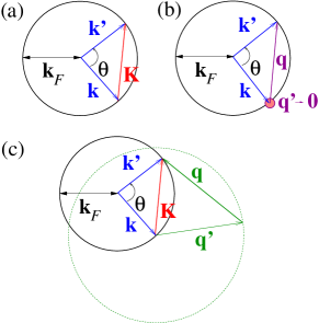
Figure 1: Scattering of electrons in momentum space due to: (a) in-plane phonons, (b) non-strained flexural and (c) strained flexural phonons.

In the low $T$ regime, $T\ll T_{BG}$, we have $z_{\nu}\gg 1$, so that the integrand in Eq. (42) is only contributing significantly for $x\ll 1$. The generalized electron–in-plane phonon coupling in (43) then becomes,

$$D_{B}^{\nu}(y\ll 1)=\left[2g^{2}y^{2}\delta_{\nu L}+\frac{\hbar^{2}v_{F}^{2}\beta^{2}}{4a^{2}}\right]^{1/2},$$ (44)

and the resistivity reads,

$$\varrho_{in}\approx\sum_{\nu}\left[g^{2}\frac{16\Gamma(6)\zeta(6)}{\Gamma(4)\zeta(4)}\left(\frac{T}{T_{BG}}\right)^{2}\delta_{\nu L}+\frac{\hbar^{2}v_{F}^{2}\beta^{2}}{4a^{2}}\right]\times\\ \frac{\Gamma(4)\zeta(4)(k_{B}T)^{4}}{e^{2}\rho\hbar^{4}v_{F}^{2}v_{\nu}^{5}k_{F}^{3}},$$ (45)

where $\Gamma(n)=(n-1)!$ is the gamma function and $\zeta(n)$ is the Riemann zeta function. We have thus obtained the expected $T^{4}$ behavior at low $T$ for coupling through gauge potential, which is the 2–dimensional analogue of the $T^{5}$ Bloch theory in 3–dimensional metals.Ziman (1960); Hwang and Sarma (2008) The scalar potential contribution comes proportional to $T^{6}$ due to screening. It can be neglected in the low $T$ regime; even though $16\Gamma(6)\zeta(6)/[\Gamma(4)\zeta(4)]\approx 300$, it is strongly suppressed by $T/T_{BG}\ll 1$ and $g<\hbar v_{F}\beta/(2a)$, (see Sec. III.2).

In the high $T$ regime, $T\gg T_{BG}$, the inequality $z_{\nu}\ll 1$ holds, so that $e^{z_{\nu}x}/(e^{z_{\nu}x}-1)^{2}\approx 1/(z_{\nu}x)$ in Eq. (42). The usual linear in $T$ resistivity for one phonon scattering is then recovered,

$$\varrho_{in}\approx\left(7g^{2}+\frac{\hbar^{2}v_{F}^{2}\beta^{2}}{8a^{2}}\frac{v_{L}^{2}}{\bar{v}^{2}}\right)\frac{\pi k_{B}T}{4\hbar\rho e^{2}v_{L}^{2}v_{F}^{2}},$$ (46)

where $1/\bar{v}^{2}=1/v_{L}^{2}+1/v_{T}^{2}$. Note that, at odds with the low $T$ regime, now the scalar potential contribution is higher than the gauge potential one for the typical coupling values discussed in Sec. III.2.

The monolayer case has been discussed extensively in the literature.Hwang and Sarma (2008); Stauber et al. (2007); Mariani and von Oppen (2008, 2010); Castro et al. (2010) The resistivity is still given by Eq. (42), only the generalized electron–in-plane phonon coupling changes,

$$D_{M}^{\nu}(y)=\left[2g^{2}y^{2}\left(1-\frac{y^{2}}{4}\right)\delta_{\nu L}+\frac{\hbar^{2}v_{F}^{2}\beta^{2}}{4a^{2}}\right]^{1/2}.$$ (47)

The same qualitative behavior is obtained: at low $T$ the resistivity is given by Eq. (45) with the numerical replacement $16\rightarrow 12$ in the scalar potential contribution; at high $T$ the result (46) holds with the replacement $\left(7g^{2}+\frac{\hbar^{2}v_{F}^{2}\beta^{2}}{8a^{2}}\frac{v_{L}^{2}}{\bar{v}^{2}}\right)\rightarrow\left(2g^{2}+\frac{\hbar^{2}v_{F}^{2}\beta^{2}}{2a^{2}}\frac{v_{L}^{2}}{\bar{v}^{2}}\right)$. Note, however, the apparent quantitative difference: the scalar and gauge potential contributions change roles, the later becoming more important in monolayer graphene. This is further discussed in Sec. V.

A final remark regarding the temperature dependent resistivity due to in-plane phonons has to do with the value of the electron-phonon coupling parameters $\beta$ and $g$. While $\beta$ is expected to be restricted to the range $\beta\sim 2-3$, as discussed in Sec. III.2, the value of the deformation potential parameter $g$ is still debated in the literature. Phenomenology gives $g\sim 10-30\,\,\mbox{eV}$;Suzuura and Ando (2002); Hwang and Sarma (2008) recent ab initio calculations provide a much smaller value $g\sim 3\,\,\mbox{eV}$.Choi et al. (2010) On the other hand, experiments seem to confirm the higher values, giving $g\sim 15-25\,\,\mbox{eV}$.Chen et al. (2008); Efetov and Kim (2010) Our claim here is that all these values make sense, if properly interpreted: phenomenology gives essentially unscreened deformation potential, which we called $g_{0}$ in Sec. III.2, and which should take values of $\mathcal{O}(10)\,\,\mbox{eV}$; screening effects suppress the deformation potential to $\mathcal{O}(1)\,\,\mbox{eV}$, as we have seen in Sec. III.2 within the Thomas Fermi approximation, in good agreement with ab initio results where screening is built in; the fact that transport experiments give a much higher deformation potential is a strong indication that phonon scattering through gauge potential, usually not included when fitting the data,Chen et al. (2008); Efetov and Kim (2010) is at work. Indeed, using the monolayer version of Eq. (46), we readily find that the fitting quantity in Refs. Chen et al., 2008 and Efetov and Kim, 2010 should be replaced by,

$$\tilde{D}=\left[2g^{2}+\frac{v_{F}^{2}\hbar^{2}\beta^{2}}{2a^{2}}\left(1+\frac{v_{L}^{2}}{v_{T}^{2}}\right)\right]^{1/2},$$ (48)

which, keeping $g\sim 3\,\,\mbox{eV}$, takes values $\tilde{D}\sim 10-20\,\,\mbox{eV}$ for $\beta\sim 2-3$, in excellent agreement with experiments. Moreover, since the gauge potential is not screened [Eq. (45)] it provides a natural explanation for the $T^{4}$ resistivity behavior recently reported at low $T$ in Ref. Efetov and Kim, 2010, where the expected $T^{6}$ contribution due to scalar potential is absent.Min et al.

Typical $T$ dependent resistivity due to scattering by in-plane phonons, Eq. (42), is shown in Fig. 2 as thick dashed lines. In agreement with analytical results, there is no qualitative difference between monolayer graphene [Fig. 2(a)] and bilayer [Fig. 2(b)].

IV.3.2 Scattering by non-strained flexural phonons

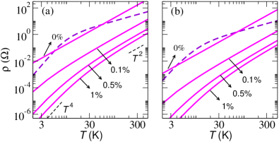
Figure 2: Resistivity vs $T$ due to scattering by in-plane phonons (dashed thick lines) and flexural phonons (full lines) with and without strain (indicated in percentage), in monolayer (a) and bilayer graphene (b). We use $n=10^{12}\,\mbox{cm}^{-2}$, $g\approx 3\,\mbox{eV}$, and $\beta\approx 3$.

In non-strained bilayer graphene scattering by FPs give rise to the following $T$ dependent resistivity (details on the derivation are given in Appendix C.2),

$$\varrho_{F}\approx\frac{\hbar k_{F}^{2}}{2\pi e^{2}\rho^{2}v_{F}^{2}\alpha^{2}}\ln\left(\frac{k_{B}T}{\hbar\alpha q_{c}^{2}}\right)\int_{0}^{1}dx\frac{[D_{B}^{F}(2x)]^{2}}{\sqrt{1-x^{2}}}\frac{x^{4}e^{zx^{2}}}{(e^{zx^{2}}-1)^{2}},$$ (49)

where $z=\hbar\omega_{2k_{F}}^{F}/k_{B}T$, and where the generalized electron–FP coupling for bilayer graphene is given by,

$$D_{B}^{F}(x)=\left[g^{2}x^{2}\left(1-\frac{x^{2}}{2}\right)^{2}+\frac{\hbar^{2}v_{F}^{2}\beta^{2}}{4a^{2}}\left(1-\frac{x^{2}}{4}\right)\right]^{1/2}.$$ (50)

Equation (49) holds also for monolayer graphene, we need only to introduce a different generalized electron-FP coupling,

$$D_{M}(x)=\left[g^{2}x^{2}\left(1-\frac{x^{2}}{4}\right)+\frac{\hbar^{2}v_{F}^{2}\beta^{2}}{4a^{2}}\right]^{1/2}.$$ (51)

In Fig. 1(b) a sketch of the two phonon scattering process in momentum space is provided. It shows that one of the two phonons involved in the scattering event always has momentum $\mathbf{q}^{\prime}\rightarrow 0$. This is a consequence of the quadratic FP dispersion [Eq. (4)], which leads to a divergent number of FPs with momentum $\mathbf{q}^{\prime}\rightarrow 0$.Castro Neto et al. (2009) This divergence is responsible for the logarithmic factor in Eq. (49), which stems from the existence of an infrared cutoff $q_{c}$. This cutoff is to be identified with the onset of anharmonic effects,Zakharchenko et al. (2010b) or unavoidable built in strain.Castro et al. (2010)

In the low $T$ regime, $T\ll T_{BG}$, one has $z\gg 1$, so that the integrand in Eq. (49) is only contributing for $x\ll 1$. The generalized electron-phonon coupling becomes equal in both bilayer and monolayer systems,

$$D_{B}(y\ll 1)=D_{M}(y\ll 1)=\left[g^{2}y^{2}+\frac{\hbar^{2}v_{F}^{2}\beta^{2}}{4a^{2}}\right]^{1/2},$$ (52)

and the resistivity is then the same in both,

$$\varrho_{F}\approx\left[g^{2}\frac{6\Gamma(6)\zeta(6)}{\Gamma(4)\zeta(4)}\left(\frac{T}{T_{BG}}\right)^{2}+\frac{\hbar^{2}v_{F}^{2}\beta^{2}}{4a^{2}}\right]\times\\ \frac{\Gamma(4)\zeta(4)\hbar k_{F}^{2}}{2^{4}\pi e^{2}\rho^{2}v_{F}^{2}\alpha^{2}}\left(\frac{k_{B}T}{\hbar\alpha k_{F}^{2}}\right)^{5/2}\ln\left(\frac{k_{B}T}{\hbar\alpha q_{c}^{2}}\right).$$ (53)

A similar result has been derived in Ref. Mariani and von Oppen, 2008. Owing to the same arguments used in the previous section for one phonon scattering we can neglect the scalar potential contribution at low $T$.

At high $T$, i.e. $T\gg T_{BG}$, we have $z\ll 1$, so that $\exp(zx^{2})/[\exp(zx^{2})-1]^{2}\approx 1/(zx^{2})$ in Eq. (49). The bilayer graphene resistivity becomes,

$$\varrho_{F}\approx\left(g^{2}+\frac{\hbar^{2}v_{F}^{2}\beta^{2}}{8a^{2}}\right)\frac{(k_{B}T)^{2}}{64\hbar e^{2}\rho^{2}v_{F}^{2}\alpha^{4}k_{F}^{2}}\ln\left(\frac{k_{B}T}{\hbar\alpha q_{c}^{2}}\right).$$ (54)

This result holds for monolayer graphene with the substitution $\left(g^{2}+\frac{\hbar^{2}v_{F}^{2}\beta^{2}}{8a^{2}}\right)\rightarrow\left(\frac{g^{2}}{2}+\frac{\hbar^{2}v_{F}^{2}\beta^{2}}{4a^{2}}\right)$.Mariani and von Oppen (2010); Castro et al. (2010) We have obtained that the resistivity due to non-strained FPs is proportional to $T^{2}/n$, which implies mobility independent of the carrier density $n$. A similar result has been obtained in the context of microscopic ripples in graphene.Katsnelson and Geim (2008); Morozov et al. (2008) The result of Eq. (54) is shown in Fig. 2(b) as a full line indicating $\bar{u}\approx 0\%$. The logarithmic correction, expected to be of order unity in the relevant $T$ range, has been ignored. Scattering by FPs dominates the contribution to resistivity in non-strained samples at both low and high $T$, except for the crossover region where $T\sim T_{BG}$, Eq. (39). The same conclusion holds for monolayer graphene, whose $T$ dependent $\varrho_{F}$ is shown in Fig. 2(a).

IV.3.3 Scattering by strained flexural phonons

Applying strain breaks the membrane rotational symmetry inducing linear FP dispersion at low momentum, as can be seen in Eq. (8). A new energy scale appears in the problem,

$$\omega_{q^{*}}^{F}=\sqrt{2}\bar{u}v_{L}^{2}/\alpha\approx 10^{4}\bar{u}(\mbox{K}),$$ (55)

separating two regimes: linear dispersion below and quadratic dispersion above. The associated momentum scale, $q^{*}=\sqrt{\bar{u}}v_{L}/\alpha\approx 4.5\sqrt{\bar{u}}\,\,\mbox{\AA}^{-1}$, together with $k_{F}$ and the thermal momentum $q_{T}$ given by $\hbar\omega_{q_{T}}^{F}=k_{B}T$, define all regimes where analytic treatment can be employed. In particular, in the low $T$ regime where $q_{T}\ll k_{F}$ we may always take $q^{*}\gg q_{T}$ and use a linear dispersion for FPs; otherwise the non strained case considered in the previous section would be the appropriate starting point. In the high $T$ regime we can distinguish between low strain for $q^{*}\ll q_{T}$ and high strain for $q^{*}\gg q_{T}$. Note that at high $T$ relevant phonons scattering electrons have momentum $q$ in the range $k_{F}\lesssim q\lesssim q_{T}$. Therefore, when strain is present in the high $T$ regime we may always assume $q^{*}\gg k_{F}$; the opposite limit, $q^{*}\ll k_{F}$, would again be identified with the non-strained case considered previously.

The resistivity due to strained FPs can be cast in the form of a triple integral over rescaled momenta $x\rightarrow\tilde{x}=x\hbar v_{L}u^{1/2}/(k_{B}T)$ (see Appendix C.2 for details),

$$\varrho_{F}\approx\frac{(k_{B}T)^{6}}{2^{6}\pi^{2}\hbar^{5}e^{2}\rho^{2}v_{F}^{2}v_{L}^{8}\bar{u}^{4}k_{F}^{2}}\int_{0}^{2\tilde{k}_{F}}d\tilde{K}\frac{[D_{B}^{F}(\tilde{K}/\tilde{k}_{F})]^{2}\tilde{K}^{2}}{\sqrt{\tilde{k}_{F}^{2}-\tilde{K}^{2}/4}}\int_{0}^{\infty}d\tilde{q}\,\frac{\tilde{q}^{3}}{\omega_{\tilde{q}}}n_{\tilde{q}}(n_{\tilde{q}}+1)\times\\ \int_{|\tilde{K}-\tilde{q}|}^{|\tilde{K}+\tilde{q}|}d\tilde{Q}\frac{\tilde{Q}^{3}n_{\tilde{Q}}(n_{\tilde{Q}}+1)}{\omega_{\tilde{Q}}\sqrt{\tilde{q}^{2}\tilde{K}^{2}-\Bigl{(}\tilde{K}^{2}+\tilde{q}^{2}-\tilde{Q}^{2}\Bigr{)}^{2}/4}}\left(\frac{\omega_{\tilde{q}}+\omega_{\tilde{Q}}}{1+n_{\tilde{q}}+n_{\tilde{Q}}}-\frac{\omega_{\tilde{q}}-\omega_{\tilde{Q}}}{n_{\tilde{q}}-n_{\tilde{Q}}}\right),$$ (56)

where the rescaled dispersion reads $\omega_{\tilde{x}}\approx\sqrt{\gamma^{2}\tilde{x}^{4}+\tilde{x}^{2}}$, with $\gamma=\sqrt{2}\omega_{q_{T}}^{F}/\omega_{q^{*}}^{F}$, and the generalized electron-FP coupling $D_{B}^{F}(y)$ is given by Eq. (50). For monolayer graphene only the coupling changes, being given instead by Eq. (51). The kinematics of the scattering process is schematically shown in Fig. 1(c).

In the low $T$ case, $T\ll T_{BG}$, we have only small angle scattering with $K\ll k_{F}$. The argument of the generalized electron-FP coupling becomes small, $K/k_{F}\ll 1$, and it can be written as

$$D_{B}(y\ll 1)\approx D_{M}(y\ll 1)\approx\left[g^{2}y^{2}+\frac{\hbar^{2}v_{F}^{2}\beta^{2}}{4a^{2}}\right]^{1/2}.$$ (57)

The resistivity is the same in both bilayer and monolayer systems. Since the inequality $q_{T}\ll k_{F},q^{*}$ holds, relevant phonons have linear dispersion $\omega_{q}^{F}\approx\sqrt{\bar{u}}v_{L}q$ and the rescaled Fermi momentum obeys $\tilde{k}_{F}\approx k_{F}/q_{T}\gg 1$. We may take $\tilde{K}\rightarrow\infty$ as the upper limit in the $\tilde{K}$ integral in Eq. (56), and the resistivity is then approximated by,

$$\varrho_{F}\approx\left[g^{2}\left(\frac{q_{T}}{k_{F}}\right)^{2}\mathcal{K}_{4}+\frac{\hbar^{2}v_{F}^{2}\beta^{2}}{4a^{2}}\mathcal{K}_{2}\right]\frac{(k_{B}T)^{7}}{2^{6}\pi^{2}\hbar^{6}e^{2}\rho^{2}v_{F}^{2}v_{L}^{9}\bar{u}^{9/2}k_{F}^{3}},$$ (58)

where

$$\mathcal{K}_{n}=\int_{0}^{\infty}d\tilde{K}\tilde{K}^{n}\int_{0}^{\infty}d\tilde{q}\,q^{2}n_{\tilde{q}}(n_{\tilde{q}}+1)\times\\ \int_{|\tilde{K}-\tilde{q}|}^{|\tilde{K}+\tilde{q}|}d\tilde{Q}\frac{\tilde{Q}^{2}n_{\tilde{Q}}(n_{\tilde{Q}}+1)\left(\frac{\tilde{q}+\tilde{Q}}{1+n_{\tilde{q}}+n_{\tilde{Q}}}-\frac{\tilde{q}-\tilde{Q}}{n_{\tilde{q}}-n_{\tilde{Q}}}\right)}{\sqrt{\tilde{q}^{2}\tilde{K}^{2}-\Bigl{(}\tilde{K}^{2}+\tilde{q}^{2}-\tilde{Q}^{2}\Bigr{)}^{2}/4}}.$$ (59)

It can be shown numerically that $\mathcal{K}_{2}\approx 4485$ and $\mathcal{K}_{4}\approx 496850$. The large ratio $\mathcal{K}_{4}/\mathcal{K}_{2}\gg 1$ is, however, compensated by $q_{T}/k_{F}\ll 1$ and the fact that $g<\hbar v_{F}\beta/(2a)$ (see Sec. III.2). As in the case of scattering by in-plane phonons, also here the gauge potential contribution to resistivity dominates at low $T$.

Now we consider the high $T$ regime, $T\gg T_{BG}$. At odds with the non-strained case [see Fig. 1(b)], now phonons with momentum $q$ in the range $k_{F}\lesssim q\lesssim q_{T}$ provide most of the scattering. It is shown in Appendix C.2.2 that the integral over $\tilde{Q}$ in Eq. (56) becomes $\tilde{K}$ independent, and the $\tilde{q}$ integral can be cast in the form,

$$\mathcal{G}(\gamma)=\int_{0}^{\infty}d\tilde{q}\,\frac{\tilde{q}^{5}n_{\tilde{q}}^{2}(n_{\tilde{q}}+1)^{2}}{\gamma^{2}\tilde{q}^{4}+\tilde{q}^{2}}\left(\frac{2\sqrt{\gamma^{2}\tilde{q}^{4}+\tilde{q}^{2}}}{1+2n_{\tilde{q}}}+\frac{1}{n_{\tilde{q}}(n_{\tilde{q}}+1)}\right),$$ (60)

being easily evaluated numerically. The resistivity in bilayer graphene can then be written as

$$\varrho_{F}\approx\left(7g^{2}+\frac{\hbar^{2}v_{F}^{2}\beta^{2}}{4a^{2}}\right)\frac{(k_{B}T)^{4}}{2^{7}\hbar^{3}e^{2}\rho^{2}v_{F}^{2}v_{L}^{6}\bar{u}^{3}}\mathcal{G}\left(\frac{\alpha k_{B}T}{\hbar\bar{u}v_{L}^{2}}\right).$$ (61)

When $\gamma\ll 1$, or equivalently $q_{T}\ll q^{*}$ (high strain), the function $\mathcal{G}(\gamma)$ behaves as $\mathcal{G}(\gamma\ll 1)\approx 18\zeta(3)-93\zeta(5)/8$. For $\gamma\gg 1$, or equivalently $q_{T}\gg q^{*}$ (small strain), it gives $\mathcal{G}(\gamma\gg 1)\approx 1/\gamma^{2}$. In these asymptotic regimes one can obtain analytic expressions for the resistivity in Eq. (61),

$$\varrho_{F}\approx\left(7g^{2}+\frac{\hbar^{2}v_{F}^{2}\beta^{2}}{4a^{2}}\right)\frac{1}{2^{7}\hbar^{3}e^{2}v_{F}^{2}}\times\\ \begin{cases}\left(18\zeta(3)-\frac{93}{8}\zeta(5)\right)\frac{(k_{B}T)^{4}}{\rho^{2}v_{L}^{6}\bar{u}^{3}}&k_{F}\ll q_{T}\ll q^{*}\\ \frac{\hbar^{2}(k_{B}T)^{2}}{\rho\kappa v_{L}^{2}\bar{u}}&k_{F}\ll q^{*}\ll q_{T}\end{cases}.$$ (62)

Equations (61) and (62) also hold for monolayer graphene with $\left(7g^{2}+\frac{\hbar^{2}v_{F}^{2}\beta^{2}}{4a^{2}}\right)\rightarrow\left(2g^{2}+\frac{\hbar^{2}v_{F}^{2}\beta^{2}}{a^{2}}\right)$.

The effect of strain in the $T$ dependence of resistivity is shown in Fig. 2(a) for monolayer graphene and 2(b) for bilayer at strain values $\bar{u}\approx 0.1\%,0.5\%,1\%$. The crossover between the two regimes of Eq. (61) [see Eq. (62)] is clearly seen at $\gamma\approx 1$, which is equivalent to $T\approx 10^{4}\bar{u}\,\,\mbox{K}$. It is apparent from Fig. 2 that the contribution to the resistivity due to scattering by FPs is strongly suppressed by applying strain.

IV.4 Crossover between in-plane and flexural phonon dominated scattering

Scattering by in-plane and flexural phonons are always at work simultaneously. However, the two mechanisms provide completely different $T$ dependent resistivity, and therefore we expect them to dominate at different $T$. In the following we address the transition $T$ at which $\varrho_{in}\approx\varrho_{F}$.

IV.4.1 Non-strained case

In this case, using Eqs. (46) and (54) for bilayer graphene in the high $T$ regime we get

$$\frac{\varrho_{F}}{\varrho_{in}}\approx\frac{T[K]}{75n[\mbox{cm}^{-2}]},$$ (63)

We expect a crossover between in-plane to FP dominated scattering given by

$$T_{c2}\approx 75n[\mbox{cm}^{-2}]\,\,\mbox{K}.$$ (64)

The $T_{c}$ just obtained is close to $T_{BG}$ for in-plane phonons, Eq. (39), and much higher than $T_{BG}$ for FPs, Eq. (40). Using the low $T$ approximation for $\varrho_{in}$, Eq. (45), we obtain the ratio

$$\frac{\varrho_{F}}{\varrho_{in}}\approx 12\frac{\sqrt{n[\mbox{cm}^{-2}]}}{(T[\mbox{K}])^{2}},$$ (65)

from which we expect a crossover from FP to in-plane dominated scattering at

$$T_{c1}\approx 3(n[\mbox{cm}^{-2}])^{1/4}\,\,\mbox{K},$$ (66)

as $T$ increases. We conclude that scattering by FP always dominates over scattering by in-plane ones, except for the region $T_{c1}\ll T\ll T_{c2}$ around $T_{BG}$ for in-plane phonons, Eq. (39). This is clearly seen in Fig. 2(b). The same conclusion applies to monolayer graphene. In this later case we obtain $T_{c1}\approx 6(n[\mbox{cm}^{-2}])^{1/4}\,\,\mbox{K}$ and $T_{c2}\approx 55n[\mbox{cm}^{-2}]\,\,\mbox{K}$.

IV.4.2 Strained case

It can easily be shown that the crossover from in-plane to flexural phonon dominated scattering always occurs in the low strain regime, $q^{*}\ll q_{T}$. We have seen in the previous sections that the crossover temperature $T$ separating high strain from low strain behavior is given by $\gamma=\sqrt{2}\omega_{q_{T}}^{F}/\omega_{q^{*}}^{F}\approx 1$. Using Eq. (55) we get a crossover temperature $T^{*}\approx 10^{4}\bar{u}\,\mbox{K}$. On the other hand, using the low strain approximation for the resistivity due to flexural phonons given in Eq. (62) and the resistivity due to in-plane ones in Eq. (46) we obtain for the ratio in bilayer graphene

$$\frac{\varrho_{F}}{\varrho_{in}}\approx\frac{k_{B}T}{40\pi\kappa\bar{u}}.$$ (67)

The corresponding crossover $T$ then reads

$$T_{c}\approx 10^{6}\bar{u}\,\mbox{K}.$$ (68)

Clearly $T_{c}\gg T^{*}$, justifying our low strain approximation. The same applies to monolayer graphene under strain. The resistivity ratio is in that case $\varrho_{F}/\varrho_{in}\approx k_{B}T/(50\pi\kappa\bar{u})$, from which we obtain roughly the same $T_{c}$ even taken into account that $\kappa$ in monolayer is half that of bilayer in our elasticity model.

In important conclusion may be drawn. While in the non-strained case scattering by FP is the dominant contribution to the resistivity, it can be seen from Eq. (68) that applying small amounts of strain is enough to suppress this contribution at room $T$. This is clearly seen in Fig. 2.

V Discussion

We have found the $T$ dependent resistivity due to acoustic phonons to be qualitatively similar in monolayer and bilayer graphene (see Sec. IV.3). This becomes apparent when we compare Fig. 2(a) and 2(b) where $\varrho(T)$ is shown, respectively, for monolayer and bilayer graphene both at zero and finite strain. Such behavior can be traced back to the resistivity expression, Eq. (36), or more precisely to its numerator, where the different electronic structure and electron-phonon coupling conspire to give exactly the same parametric dependence in monolayer and bilayer graphene. In short, it can be readily seen through Eq. (36) that the information about the electronic structure enters via the density of states squared in the numerator. The electron-phonon coupling, in its turn, enters through the transition rate $\mathcal{P}_{\mathbf{k},\mathbf{k}^{\prime}}$, and in the Born approximation it also appears squared. When coupling is via scalar potential [$V_{1}$ matrix elements in Eq. (23)] the screening makes the coupling inversely proportional to the density of states, and the square of it cancels exactly with the square density of states coming from the integral over $\mathbf{k}$ and $\mathbf{k}^{\prime}$ in the numerator of Eq. (36). For the coupling through gauge potential [$V_{2}$ matrix elements in Eq. (23)] the parametric difference between monolayer and bilayer amounts to the replacement $v_{F}^{2}\rightarrow\hbar^{2}k_{F}^{2}/(2m)^{2}$ (after taking the square of the matrix elements and using the quasielastic approximation). When multiplied by the square of the density of states in bilayer graphene, $\mathcal{D}(E)\sim m/\hbar^{2}$, we obtain the factor $k_{F}^{2}/\hbar^{2}$, which has exactly the same parametric dependence appearing for single layer graphene – there, the factor $v_{F}^{2}$ multiplies the square of the density of states of the monolayer, $\mathcal{D}(E)\sim k/(\hbar v_{F})$.

Despite qualitative similarities there are apparent quantitative differences. A striking one is the overall suppression of resistivity in bilayer graphene, which is clearly seen when we compare Fig. 2(a) and 2(b). This is due to the higher stiffness and mass density of bilayer graphene (see Sec. II), and to the $1/2$ term in Eq. (17) for the gauge potential which, at odds with the parametric dependence just discussed, does not cancel out in the expression for the resistivity. Also, the scalar potential contribution is quantitative different, being enhanced in bilayer graphene, as can be seen by comparing Eqs. (45), and (46), Eqs. (53) and (54), and Eqs. (58) and (61) with their monolayer counterparts. This arises because pseudo-spin conservation allows back scattering due to scalar potential in bilayer but not in monolayer graphene.

The quantitative discrepancy between the $T$ dependent resistivity in bilayer and monolayer graphene originates an interesting difference regarding room $T$ mobility in non-strained samples. The mobility $\mu$, defined as $\varrho=1/(en\mu)$, is in the non-strained case limited by PF scattering (see Sec. IV.3.2) and takes the form

$$\mu\approx\mathcal{A}\frac{64\pi\hbar ev_{F}^{2}}{k_{B}^{2}T^{2}},$$ (69)

with $\mathcal{A}_{B}=\kappa^{2}/[g^{2}+\hbar^{2}v_{F}^{2}\beta^{2}/(8a^{2})]$ in bilayer graphene and $\mathcal{A}_{M}=\kappa^{2}/[g^{2}/2+\hbar^{2}v_{F}^{2}\beta^{2}/(4a^{2})]$ in monolayer graphene, ignoring the logarithmic contribution of order unity, Eq. (54). For monolayer graphene at room $T$ the mobility is limited to the value for samples on substrate, $\mu\approx 198\mathcal{A}_{M}\sim 1\,\,\mbox{m}^{2}/\mbox{Vs}$, as has recently been confirmed experimentally.Castro et al. (2010) For bilayer graphene, however, the quantitative differences discussed above lead to an enhanced room $T$ mobility, $\mu\approx 198\mathcal{A}_{B}\sim 20\,\,\mbox{m}^{2}/\mbox{Vs}$. This might be an interesting aspect to take into account regarding room $T$ electronic applications. Reports of much smaller mobility (one order of magnitude) in recent experiments in suspended bilayer grapheneFeldman et al. (2009) might be an indication that residual, $T$ independent scattering is at work, overcoming the intrinsic FP contribution.

Another remark worth discussion is the validity of results in the non-strained regime, in particular Eq. (54) for the high $T$ resistivity. At low densities, when $k_{F}$ becomes comparable with the infrared cutoff $q_{c}$ given by the onset of anharmonic effects,Zakharchenko et al. (2010b) the harmonic approximation used here breaks down. A complete theory would require taking into account anharmonicities, but this is beyond the scope of the present work. Nevertheless, it is likely that unavoidable little strain $u$ is always present in real samples,Castro et al. (2010) and this increases the validity of the harmonic approximation.Roldán et al. Moreover, the infrared cutoff $q_{c}$ due to anharmonic effects depends on the applied strain (see Appendix D), decreasing as strain increases. This is consistent with sample to sample mobility differences of order unity recently reported in suspended monolayer graphene,Castro et al. (2010) where strain $u\lesssim 10^{-4}-10^{-3}$ is naturally expected.

Finally, we comment on a recent theory paper by Mariani and von OppenMariani and von Oppen (2010) where the $T$ dependent resistivity of monolayer graphene has been fully discussed. In the high $T$ regime, $T\gg T_{BG}$, our results for the monolayer case agree with those of Ref. Mariani and von Oppen, 2010. However, at low $T$, i.e. $T\ll T_{BG}$, the authors of Ref. Mariani and von Oppen, 2010 found a new regime where the scalar potential contribution dominates. This happens because in Ref. Mariani and von Oppen, 2010 the electron-phonon coupling from scalar potential is assumed to be much higher than the gauge potential coupling, unless $T\ll T_{GD}$, where $T_{GD}$ is the energy scale at which screening becomes relevant and scalar and gauge potentials become comparable. The new regime arises for $T_{GD}\ll T\ll T_{BG}$. With the parameter values used in the present work, however, the electron-phonon coupling due to scalar potential is always similar or smaller than the gauge potential (see Sec. III.2). Therefore, we can neglect this low $T$ contribution since it gives higher power law behavior than the gauge potential. Recent $T$ dependent resistivity due to in-plane phonons measured in single layer graphene at the high densitiesEfetov and Kim (2010) seem to corroborate the latter picture.

VI Conclusions

In the present work we have studied the $T$ dependent resistivity due to scattering by both acoustic in-plane phonons and FPs in doped, suspended bilayer graphene. We have found the bilayer membrane to follow the qualitative behavior of the monolayer cousin.Mariani and von Oppen (2010); Castro et al. (2010) Different electronic structure combine with different electron-phonon coupling to give the same parametric dependence in resistivity, and in particular the same $T$ behavior. In parallel with the single layer, FPs dominate the phonon contribution to resistivity in the absence of strain, where a density independent mobility is obtained. This contribution is strongly suppressed by tension, similarly to monolayer graphene.Castro et al. (2010) However, an interesting quantitative difference with respect to suspended monolayer has been found. In the latter, as shown in Ref. Castro et al., 2010, FPs limit room $T$ mobility $\mu$ to values obtained for samples on substrate, $\mu\sim 1\,\,\mbox{m${}^{2}/$(Vs)}$, when tension is absent. In bilayer, quantitative differences in electron-phonon coupling and elastic constants lead to a room $T$ mobility enhanced by one order of magnitude, $\mu\sim 20\,\,\mbox{m${}^{2}/$(Vs)}$, even in non-strained samples. This finding has obvious advantages for room $T$ electronic applications. It has also been shown that for a correct description of acoustic phonon scattering in both monolayer and bilayer graphene, even at the qualitative level, coupling to both scalar and gauge potentials needs to be taken into account.

Appendix A Collision integral

The rate of change of $f_{\mathbf{k}}$ due to scattering, the so-called collision integral $\dot{f}_{\mathbf{k}}\bigr{|}_{\mathrm{scatt}}$ appearing on the right hand side of the Boltzmann equation Eq. (24), is the difference between the rate at which quasiparticles enter the state $\bigl{|}\mathbf{k}\bigr{\rangle}$ and the rate at which they leave it,

$$\dot{f}_{\mathbf{k}}\bigr{|}_{\mathrm{scatt}}=\sum_{\mathbf{k}^{\prime}}\left[f_{\mathbf{k}^{\prime}}(1-f_{\mathbf{k}})\mathcal{W}_{\mathbf{k}^{\prime}}^{\mathbf{k}}-f_{\mathbf{k}}(1-f_{\mathbf{k}^{\prime}})\mathcal{W}_{\mathbf{k}}^{\mathbf{k}^{\prime}}\right],$$ (70)

where $\mathcal{W}_{i}^{f}$ is the scattering probability between state $\bigl{|}i\bigr{\rangle}$ and $\bigl{|}f\bigr{\rangle}$. Here we use Fermi’s golden rule, which reads

$$\mathcal{W}_{i}^{f}=\frac{2\pi}{\hbar}\Bigl{|}\bigl{\langle}f\bigr{|}\mathcal{H}_{int}\bigl{|}i\bigr{\rangle}\Bigr{|}^{2}\delta(\mathcal{E}_{f}-\mathcal{E}_{i}),$$ (71)

and is equivalent to rest upon the Born approximation for the differential scattering cross-section. In this appendix we provide explicit expressions for the integral collision Eq. (70) arising due to scattering by phonons in bilayer graphene (and also monolayer for comparison).

The crucial step to get $\dot{f}_{\mathbf{k}}\bigr{|}_{\mathrm{scatt}}$ is finding the scattering probability for a quasi-particle in state $\left|\mathbf{k}\right\rangle$ to be scattered into state $\left|\mathbf{k}^{\prime}\right\rangle$, i.e. $\mathcal{W}_{\mathbf{k}}^{\mathbf{k}^{\prime}}$ (since the process is quasi-elastic interband transitions are not allowed, meaning that both states belong to the same band). The scattering mechanism is encoded in the interaction $\mathcal{H}_{int}$, which in the present case is given by $H_{ep}$ in Eq. (22). It is readily seen that scattering occurs only through emission or absorption of one phonon or emission/absorption of two phonons. The initial and final states are thus tensorial products of the form $\left|i\right\rangle=\left|\mathbf{k}\right\rangle\otimes\left|n_{\mathbf{q}}\right\rangle$ or $\left|i\right\rangle=\left|\mathbf{k}\right\rangle\otimes\left|n_{\mathbf{q}},n_{\mathbf{q^{\prime}}}\right\rangle$, and $\left|f\right\rangle=\left|\mathbf{k}^{\prime}\right\rangle\otimes\left|n_{\mathbf{q}}\pm 1\right\rangle$, $\left|f\right\rangle=\left|\mathbf{k}^{\prime}\right\rangle\otimes\left|n_{\mathbf{q}}\pm 1,n_{\mathbf{q}^{\prime}}\pm 1\right\rangle$ or $\left|f\right\rangle=\left|\mathbf{k}^{\prime}\right\rangle\otimes\left|n_{\mathbf{q}}\pm 1,n_{\mathbf{q}^{\prime}}^{F}\mp 1\right\rangle$, where $\left|n_{\mathbf{q}}\right\rangle$ and $\left|n_{\mathbf{q}},n_{\mathbf{q^{\prime}}}\right\rangle$ represent one and two phonon states in the occupation number representation,Mariani and von Oppen (2008) and the electron like quasiparticle state is written according to the unitary transformation in Eq. (10) as $\left|\mathbf{k}\right\rangle=(e^{-i\theta_{\mathbf{k}}}a_{\mathbf{k}}^{\dagger}\left|0\right\rangle+e^{i\theta_{\mathbf{k}}}b_{\mathbf{k}}^{\dagger}\left|0\right\rangle)/\sqrt{2}$ (electron-hole symmetry guarantees the result is the same for both electron and hole doping).

In order to obtain $\left|\left\langle f\right|H_{ep}\left|i\right\rangle\right|^{2}$, with $\left|i\right\rangle$ and $\left|f\right\rangle$ as given above, we take the following steps. (i) Terms of the form $V_{1}V_{2}$, where $V_{1}$ stands for scalar potential and $V_{2}$ for gauge potential induced matrix elements in Eq. (23), are neglected. It is easy to show that such terms come proportional to oscillatory factors $e^{\pm i2\theta_{\mathbf{k}}}$ or $e^{\pm i2\theta_{\mathbf{k}^{\prime}}}$ (in monolayer graphene $e^{\pm i\theta_{\mathbf{k}}}$ or $e^{\pm i\theta_{\mathbf{k}^{\prime}}}$), stemming from the unitary transformation in Eq. (10). These terms can safely be neglected in doing the summation over the direction of $\mathbf{k}$ and $\mathbf{k}^{\prime}$ in the numerator of Eq. (36), keeping $\theta_{\mathbf{k},\mathbf{k}^{\prime}}$ fixed. The resistivity is then the sum of two independent contributions, originating from scalar and gauge potentials, well in the spirit of Matthiessen’s empirical rule.Ziman (1960) (ii) For the scalar potential contribution the terms $\left|V_{1,\mathbf{q}}^{\nu}e^{i(\theta_{\mathbf{k}^{\prime}}-\theta_{\mathbf{k}})}+V_{1,\mathbf{q}}^{\nu}e^{i(\theta_{\mathbf{k}^{\prime}}-\theta_{\mathbf{k}})}\right|^{2}/4$ are proportional to the overlap of states belonging to the same band $(1+\cos 2\theta_{\mathbf{k},\mathbf{k}^{\prime}})/2$, and can be written as

$$\left|V_{1,\mathbf{q}}^{\nu}\frac{e^{i(\theta_{\mathbf{k}^{\prime}}-\theta_{\mathbf{k}})}}{2}+V_{1,\mathbf{q}}^{\nu}\frac{e^{-i(\theta_{\mathbf{k}^{\prime}}-\theta_{\mathbf{k}})}}{2}\right|^{2}=\left|V_{1,\mathbf{q}}^{\nu}\right|^{2}\frac{1+\cos 2\theta_{\mathbf{k},\mathbf{k}^{\prime}}}{2}.$$ (72)

The same manipulation holds for two phonon terms, with $V_{1,\mathbf{q}}^{\nu}\rightarrow V_{1,\mathbf{q},\mathbf{q}^{\prime}}^{F}$. (iii) For the gauge potential contribution there are oscillatory terms which, owing to the argument of point (i), can be neglected,

$$\left|V_{2,\mathbf{q},\mathbf{k},\mathbf{k}^{\prime}}^{\nu}\frac{e^{i(\theta_{\mathbf{k}^{\prime}}+\theta_{\mathbf{k}})}}{2}+\Bigl{(}V_{2,-\mathbf{q},\mathbf{k},\mathbf{k}^{\prime}}^{\nu}\Bigr{)}^{*}\frac{e^{-i(\theta_{\mathbf{k}^{\prime}}+\theta_{\mathbf{k}})}}{2}\right|^{2}\simeq\\ \left|\tilde{V}_{2,\mathbf{q}}^{\nu}\right|^{2}\left(\frac{k^{2}}{2}+\frac{k^{\prime 2}}{2}+kk^{\prime}\cos\theta_{\mathbf{k},\mathbf{k}^{\prime}}\right),$$ (73)

where we used $\tilde{V}$ to express the matrix elements given in Eq. (23) for bilayer graphene without the term $(\pi_{\mathbf{k}}+\pi_{\mathbf{k}^{\prime}})$. A similar manipulation holds for two phonon terms, with $\tilde{V}_{2,\mathbf{q}}^{\nu}\rightarrow\tilde{V}_{2,\mathbf{q},\mathbf{q}^{\prime}}^{F}$.

Finally, summing over phonon momenta and doing the thermal average, we can write $\mathcal{W}_{\mathbf{k}}^{\mathbf{k}^{\prime}}$ as follows: when scattering is via one phonon,

$$\mathcal{W}_{\mathbf{k}}^{\mathbf{k}^{\prime}} =\frac{\pi}{\hbar}\sum_{\mathbf{q}}w_{\nu}(\mathbf{q},\mathbf{k},\mathbf{k}^{\prime})n_{\mathbf{q}}\delta_{\mathbf{k}^{\prime},\mathbf{k}+\mathbf{q}}\delta(\varepsilon_{\mathbf{k}^{\prime}}-\varepsilon_{\mathbf{k}}-\hbar\omega_{\mathbf{q}}^{\nu})$$

$$+ \frac{\pi}{\hbar}\sum_{\mathbf{q}}w_{\nu}(\mathbf{q},\mathbf{k},\mathbf{k}^{\prime})(n_{\mathbf{q}}+1)\delta_{\mathbf{k}^{\prime},\mathbf{k}-\mathbf{q}}\delta(\varepsilon_{\mathbf{k}^{\prime}}-\varepsilon_{\mathbf{k}}+\hbar\omega_{\mathbf{q}}^{\nu}),$$ (74)

where the first term is due to absorption and the second to emission of a single phonon; when scattering involves two phonons,

$$\mathcal{W}_{\mathbf{k}}^{\mathbf{k}^{\prime}} =\frac{\pi}{\hbar}\sum_{\mathbf{q},\mathbf{q}^{\prime}}w_{F}(\mathbf{q},\mathbf{q}^{\prime},\mathbf{k},\mathbf{k}^{\prime})n_{\mathbf{q}}n_{\mathbf{q}^{\prime}}\times$$

$$\delta_{\mathbf{k}^{\prime},\mathbf{k}+\mathbf{q}+\mathbf{q}^{\prime}}\delta(\varepsilon_{\mathbf{k}^{\prime}}-\varepsilon_{\mathbf{k}}-\hbar\omega_{\mathbf{q}}^{F}-\hbar\omega_{\mathbf{q}^{\prime}}^{F})$$

$$+ \frac{\pi}{\hbar}\sum_{\mathbf{q},\mathbf{q}^{\prime}}w_{F}(\mathbf{q},\mathbf{q}^{\prime},\mathbf{k},\mathbf{k}^{\prime})(n_{\mathbf{q}}+1)(n_{\mathbf{q}^{\prime}}+1)\times$$

$$\delta_{\mathbf{k}^{\prime},\mathbf{k}-\mathbf{q}-\mathbf{q}^{\prime}}\delta(\epsilon_{\mathbf{k}^{\prime}}-\epsilon_{\mathbf{k}}+\hbar\omega_{\mathbf{q}}^{F}+\hbar\omega_{\mathbf{q}^{\prime}}^{F})$$

$$+ \frac{2\pi}{\hbar}\sum_{\mathbf{q},\mathbf{q}^{\prime}}w_{F}(\mathbf{q},\mathbf{q}^{\prime},\mathbf{k},\mathbf{k}^{\prime})(n_{\mathbf{q}}+1)n_{\mathbf{q}^{\prime}}\times$$

$$\delta_{\mathbf{k}^{\prime},\mathbf{k}-\mathbf{q}+\mathbf{q}^{\prime}}\delta(\epsilon_{\mathbf{k}^{\prime}}-\epsilon_{\mathbf{k}}+\hbar\omega_{\mathbf{q}}^{F}-\hbar\omega_{\mathbf{q}^{\prime}}^{F}),$$ (75)

where the first term is due to absorption of two FPs, the second to emission of two FPs, and the last one comes from absorption of a single FP and emission of another one. The kernels $w_{\nu}(\mathbf{q},\mathbf{k},\mathbf{k}^{\prime})$ and $w_{F}(\mathbf{q},\mathbf{q}^{\prime},\mathbf{k},\mathbf{k}^{\prime})$ represent the sum of the right hand side of Eq. (72) with Eq. (73), as given in Eq. (34). For Monolayer graphene $\mathcal{W}_{\mathbf{k}}^{\mathbf{k}^{\prime}}$ take exactly the same form;Mariani and von Oppen (2010) only the kernels change, being given instead by Eq. (35). The collision integral may finally be put in the form,

$$\dot{f}_{\mathbf{k}}\bigr{|}_{\mathrm{scatt}} =\frac{\pi}{\hbar}\sum_{\mathbf{k}^{\prime}}\sum_{\mathbf{q},\nu}w_{\nu}(\mathbf{q},\mathbf{k},\mathbf{k}^{\prime})\times$$

$$\times \left\{\left[f_{\mathbf{k}^{\prime}}(1-f_{\mathbf{k}})n_{\mathbf{q}}-f_{\mathbf{k}}(1-f_{\mathbf{k}^{\prime}})(n_{\mathbf{q}}+1)\right]\right.$$

$$\delta_{\mathbf{k},\mathbf{k}^{\prime}+\mathbf{q}}\delta(\varepsilon_{\mathbf{k}}-\varepsilon_{\mathbf{k}^{\prime}}-\hbar\omega_{\mathbf{q}}^{\nu})$$

$$+ \left[f_{\mathbf{k}^{\prime}}(1-f_{\mathbf{k}})(n_{\mathbf{q}}+1)-f_{\mathbf{k}}(1-f_{\mathbf{k}^{\prime}})n_{\mathbf{q}}\right]$$

$$\left.\delta_{\mathbf{k},\mathbf{k}^{\prime}-\mathbf{q}}\delta(\varepsilon_{\mathbf{k}}-\varepsilon_{\mathbf{k}^{\prime}}+\hbar\omega_{\mathbf{q}}^{\nu})\right\},$$ (76)

for one phonon scattering processes, and

$$\dot{f}_{\mathbf{k}}\bigr{|}_{\mathrm{scatt}} =\frac{\pi}{\hbar}\sum_{\mathbf{k}^{\prime}}\sum_{\mathbf{q},\mathbf{q}^{\prime}}w_{F}(\mathbf{q},\mathbf{q}^{\prime},\mathbf{k},\mathbf{k}^{\prime})\times$$

$$\times \left\{\left[f_{\mathbf{k}^{\prime}}(1-f_{\mathbf{k}})(n_{\mathbf{q}}+1)(n_{\mathbf{q}^{\prime}}+1)-f_{\mathbf{k}}(1-f_{\mathbf{k}^{\prime}})n_{\mathbf{q}}n_{\mathbf{q}^{\prime}}\right]\right.$$

$$\delta_{\mathbf{k},\mathbf{k}^{\prime}-\mathbf{q}-\mathbf{q}^{\prime}}\delta(\varepsilon_{\mathbf{k}}-\varepsilon_{\mathbf{k}^{\prime}}+\hbar\omega_{\mathbf{q}}^{F}+\hbar\omega_{\mathbf{q}^{\prime}}^{F})$$

$$+ \left[f_{\mathbf{k}^{\prime}}(1-f_{\mathbf{k}})(n_{\mathbf{q}}+1)n_{\mathbf{q}^{\prime}}-f_{\mathbf{k}}(1-f_{\mathbf{k}^{\prime}})n_{\mathbf{q}}(n_{\mathbf{q}^{\prime}}+1)\right]$$

$$\delta_{\mathbf{k},\mathbf{k}^{\prime}-\mathbf{q}+\mathbf{q}^{\prime}}\delta(\varepsilon_{\mathbf{k}}-\varepsilon_{\mathbf{k}^{\prime}}+\hbar\omega_{\mathbf{q}}^{F}-\hbar\omega_{\mathbf{q}^{\prime}}^{F})$$

$$+ \left[f_{\mathbf{k}^{\prime}}(1-f_{\mathbf{k}})n_{\mathbf{q}}n_{\mathbf{q}^{\prime}}-f_{\mathbf{k}}(1-f_{\mathbf{k}^{\prime}})(n_{\mathbf{q}}+1)(n_{\mathbf{q}^{\prime}}+1)\right]$$

$$\delta_{\mathbf{k},\mathbf{k}^{\prime}+\mathbf{q}+\mathbf{q}^{\prime}}\delta(\varepsilon_{\mathbf{k}}-\varepsilon_{\mathbf{k}^{\prime}}-\hbar\omega_{\mathbf{q}}^{F}-\hbar\omega_{\mathbf{q}^{\prime}}^{F})$$

$$+ \left[f_{\mathbf{k}^{\prime}}(1-f_{\mathbf{k}})n_{\mathbf{q}}(n_{\mathbf{q}^{\prime}}+1)-f_{\mathbf{k}}(1-f_{\mathbf{k}^{\prime}})(n_{\mathbf{q}}+1)n_{\mathbf{q}^{\prime}}\right]$$

$$\left.\delta_{\mathbf{k},\mathbf{k}^{\prime}+\mathbf{q}-\mathbf{q}^{\prime}}\delta(\varepsilon_{\mathbf{k}}-\varepsilon_{\mathbf{k}^{\prime}}-\hbar\omega_{\mathbf{q}}^{F}+\hbar\omega_{\mathbf{q}^{\prime}}^{F})\right\},$$ (77)

for scattering through two FPs.

Appendix B Linearized collision integral

In this appendix we derive the linearized version of the collision integrals given in Eqs. (76) and (77). We start by expanding electron and phonon probability distributions around their equilibrium values,

$$f_{\mathbf{k}}=f_{\mathbf{k}}^{(0)}+\delta f_{\mathbf{k}},\hskip 10.00002pt\hskip 10.00002ptn_{\mathbf{q}}=n_{\mathbf{q}}^{(0)}+\delta n_{\mathbf{q}},$$ (78)

where the variations can be written as $\delta f_{\mathbf{k}}=-\frac{\partial f_{\mathbf{k}}^{(0)}}{\partial\varepsilon_{\mathbf{k}}}\varphi_{\mathbf{k}}$ [see Eq. (26)] and $\delta n_{\mathbf{q}}=-\frac{\partial n_{\mathbf{q}}^{(0)}}{\partial(\hbar\omega_{\mathbf{q}})}\chi_{\mathbf{q}}$. The linearized collision integral $\delta\dot{f}_{\mathbf{k}}\bigr{|}_{\mathrm{scatt}}$ is then obtained by expanding $\dot{f}_{\mathbf{k}}\bigr{|}_{\mathrm{scatt}}$ up to first order in the variations.Ziman (1960); Landau and Lifshitz (1981)

B.1 One phonon scattering

This case follows closely the steps outlined in Ref. Landau and Lifshitz, 1981, and for the case of monolayer graphene it has been derived in Ref. Mariani and von Oppen, 2010. Since the difference between monolayer and bilayer amounts to a different kernel $w_{\nu}(\mathbf{q},\mathbf{k},\mathbf{k}^{\prime})$ in Eqs. (76), which does not play any role in the linearization, we can directly apply the result of Ref. Mariani and von Oppen, 2010 to the present case. In order to set notation for the more elaborated case of two phonon scattering, we outline the main steps of the derivation in the following.

We first note that at equilibrium detailed balance implies $\dot{f}_{\mathbf{k}}^{(0)}\bigr{|}_{\mathrm{scatt}}=0$, from which we get the relation

$$f_{\mathbf{k}^{\prime}}^{(0)}(1-f_{\mathbf{k}}^{(0)})n_{\mathbf{q}}^{(0)}=f_{\mathbf{k}}^{(0)}(1-f_{\mathbf{k}^{\prime}}^{(0)})(n_{\mathbf{q}}^{(0)}+1),$$ (79)

which can be easily verified by direct calculation.Landau and Lifshitz (1981) Therefore, in order to get the linearized collision integral it is enough to calculate the variation,

$$\delta\left[f_{\mathbf{k}^{\prime}}(1-f_{\mathbf{k}})n_{\mathbf{q}}-f_{\mathbf{k}}(1-f_{\mathbf{k}^{\prime}})(n_{\mathbf{q}}+1)\right]=\\ (1-f_{\mathbf{k}}^{(0)})(1-f_{\mathbf{k}^{\prime}}^{(0)})(n_{\mathbf{q}}^{(0)}+1)\delta\left(\frac{f_{\mathbf{k}^{\prime}}}{1-f_{\mathbf{k}^{\prime}}}\frac{n_{\mathbf{q}}}{n_{\mathbf{q}}+1}-\frac{f_{\mathbf{k}}}{1-f_{\mathbf{k}}}\right).$$ (80)

The variations appearing on the right hand side of Eq. (80) can be computed easily by noting that

$$\delta\left(\frac{f}{1-f}\right)=\frac{\delta f}{(1-f^{(0)})^{2}}\hskip 10.00002pt\mbox{and}\hskip 10.00002pt\delta\left(\frac{f}{n+1}\right)=\frac{\delta n}{(n^{(0)}+1)^{2}}.$$ (81)

Using Eq. (79), and rewriting $\delta f_{\mathbf{k}}$ and $\delta n_{\mathbf{q}}$ as

$$\delta f_{\mathbf{k}}=f_{\mathbf{k}}^{(0)}(1-f_{\mathbf{k}}^{(0)})\frac{\varphi_{\mathbf{k}}}{k_{B}T}\hskip 10.00002pt\delta n_{\mathbf{q}}=n_{\mathbf{q}}^{(0)}(n_{\mathbf{q}}^{(0)}+1)\frac{\chi_{\mathbf{q}}}{k_{B}T},$$ (82)

it is easy to show that

$$\delta\left[f_{\mathbf{k}^{\prime}}(1-f_{\mathbf{k}})n_{\mathbf{q}}-f_{\mathbf{k}}(1-f_{\mathbf{k}^{\prime}})(n_{\mathbf{q}}+1)\right]=\\ \frac{1}{k_{B}T}f_{\mathbf{k}}^{(0)}(1-f_{\mathbf{k}^{\prime}}^{(0)})(n_{\mathbf{q}}^{(0)}+1)\left(\varphi_{\mathbf{k}^{\prime}}+\chi_{\mathbf{q}}-\varphi_{\mathbf{k}}\right).$$ (83)

The linearized collision integral may then be obtained,

$$\delta\dot{f}_{\mathbf{k}}\bigr{|}_{\mathrm{scatt}} = -\frac{\pi}{\hbar k_{B}T}\sum_{\mathbf{k}^{\prime}}\sum_{\mathbf{q},\nu}w_{\nu}(\mathbf{q},\mathbf{k},\mathbf{k}^{\prime})f_{\mathbf{k}}^{(0)}(1-f_{\mathbf{k}^{\prime}}^{(0)})(n_{\mathbf{q}}^{(0)}+1)\left(\varphi_{\mathbf{k}^{\prime}}+\chi_{\mathbf{q}}-\varphi_{\mathbf{k}}\right)\delta_{\mathbf{k},\mathbf{k}^{\prime}+\mathbf{q}}\delta(\varepsilon_{\mathbf{k}}-\varepsilon_{\mathbf{k}^{\prime}}-\hbar\omega_{\mathbf{q}}^{\nu})$$ (84)

$$- \frac{\pi}{\hbar k_{B}T}\sum_{\mathbf{k}^{\prime}}\sum_{\mathbf{q},\nu}w_{\nu}(\mathbf{q},\mathbf{k},\mathbf{k}^{\prime})(1-f_{\mathbf{k}}^{(0)})f_{\mathbf{k}^{\prime}}^{(0)}(n_{\mathbf{q}}^{(0)}+1)\left(\varphi_{\mathbf{k}^{\prime}}-\varphi_{\mathbf{k}}-\chi_{\mathbf{q}}\right)\delta_{\mathbf{k},\mathbf{k}^{\prime}-\mathbf{q}}\delta(\varepsilon_{\mathbf{k}}-\varepsilon_{\mathbf{k}^{\prime}}+\hbar\omega_{\mathbf{q}}^{\nu}).$$

Now we introduce two typical approximations: consider phonons at equilibrium by taking $\chi_{\mathbf{q}}\approx 0$, so that $n_{\mathbf{q}}\approx n_{\mathbf{q}}^{(0)}$, valid at not too low temperatures;Ziman (1960) consider quasielastic scattering, with $\varepsilon_{\mathbf{k}},\varepsilon_{\mathbf{k}^{\prime}}\gg\hbar\omega_{\mathbf{q}}$. The latter approximation enables us to rewrite the delta functions, $\delta(\varepsilon_{\mathbf{k}}-\varepsilon_{\mathbf{k}^{\prime}}\pm\hbar\omega_{\mathbf{q}}^{\nu})\rightarrow\delta(\varepsilon_{\mathbf{k}}-\varepsilon_{\mathbf{k}^{\prime}})$, and to approximate $f_{\mathbf{k}}^{(0)}(1-f_{\mathbf{k}^{\prime}}^{(0)})$ byLandau and Lifshitz (1981)

$$f_{\mathbf{k}}^{(0)}(1-f_{\mathbf{k}^{\prime}}^{(0)})=(f_{\mathbf{k}^{\prime}}^{(0)}-f_{\mathbf{k}}^{(0)})n_{\mathbf{q}}^{(0)}\approx\pm\hbar\omega_{\mathbf{q}}\frac{\partial f_{\mathbf{k}}^{(0)}}{\partial\epsilon_{\mathbf{k}}}n_{\mathbf{q}}^{(0)}.$$ (85)

The linearized collision integral then reads

$$\delta\dot{f}_{\mathbf{k}}\bigr{|}_{\mathrm{scatt}}=-\frac{2\pi}{\hbar}\sum_{\mathbf{k}^{\prime}}\sum_{\mathbf{q},\nu}w_{\nu}(\mathbf{q},\mathbf{k},\mathbf{k}^{\prime})\omega_{\mathbf{q}}^{\nu}\times\\ \frac{\partial n_{\mathbf{q}}}{\partial\omega_{\mathbf{q}}^{\nu}}\frac{\partial f_{\mathbf{k}}^{(0)}}{\partial\epsilon_{\mathbf{k}}}(\varphi_{\mathbf{k}}-\varphi_{\mathbf{k}^{\prime}})\delta_{\mathbf{k},\mathbf{k}^{\prime}+\mathbf{q}}\delta(\epsilon_{\mathbf{k}}-\epsilon_{\mathbf{k}^{\prime}}),$$ (86)

where we have used equalities $w_{\nu}(\mathbf{q},\mathbf{k},\mathbf{k}^{\prime})=w_{\nu}(-\mathbf{q},\mathbf{k},\mathbf{k}^{\prime})$ and $\omega_{\mathbf{q}}=\omega_{-\mathbf{q}}$. Finally, Eq. (86) can be put in the form of Eq. (27),

$$\dot{f}_{\mathbf{k}}\bigr{|}_{\mathrm{scatt}}=-\sum_{\mathbf{k}^{\prime}}\mathcal{P}_{\mathbf{k},\mathbf{k}^{\prime}}(\varphi_{\mathbf{k}}-\varphi_{\mathbf{k}^{\prime}}),$$ (87)

where $\mathcal{P}_{\mathbf{k},\mathbf{k}^{\prime}}$ is given in Eq. (32).

B.2 Two phonon scattering

Now we proceed with the linearization of the collision integral in Eq. (77), originating from scattering processes involving two FPs. At equilibrium detailed balance is guaranteed, $\dot{f}_{\mathbf{k}}^{(0)}\bigr{|}_{\mathrm{scatt}}=0$, and the following two relations hold,

$$\frac{f_{\mathbf{k}^{\prime}}^{(0)}}{1-f_{\mathbf{k}^{\prime}}^{(0)}} = \frac{f_{\mathbf{k}}^{(0)}}{1-f_{\mathbf{k}}^{(0)}}\frac{n_{\mathbf{q}}^{(0)}}{n_{\mathbf{q}}^{(0)}+1}\frac{n_{\mathbf{q}^{\prime}}^{(0)}}{n_{\mathbf{q}^{\prime}}+1},$$

$$\frac{f_{\mathbf{k}^{\prime}}^{(0)}}{1-f_{\mathbf{k}^{\prime}}^{(0)}}\frac{n_{\mathbf{q}^{\prime}}^{(0)}}{n_{\mathbf{q}^{\prime}}^{(0)}+1} = \frac{f_{\mathbf{k}}^{(0)}}{1-f_{\mathbf{k}}^{(0)}}\frac{n_{\mathbf{q}}^{(0)}}{n_{\mathbf{q}}^{(0)}+1}.$$ (88)

In order to get the linearized collision integral it is easy to see that we only need the following two variations,

$$\delta\left[f_{\mathbf{k}^{\prime}}(1-f_{\mathbf{k}})(n_{\mathbf{q}}+1)(n_{\mathbf{q}^{\prime}}+1)-f_{\mathbf{k}}(1-f_{\mathbf{k}^{\prime}})n_{\mathbf{q}}n_{\mathbf{q}^{\prime}}\right]=\\ (1-f_{\mathbf{k}}^{(0)})(1-f_{\mathbf{k}^{\prime}}^{(0)})(n_{\mathbf{q}}^{(0)}+1)(n_{\mathbf{q}^{\prime}}^{(0)}+1)\times\\ \delta\left(\frac{f_{\mathbf{k}^{\prime}}}{1-f_{\mathbf{k}^{\prime}}}-\frac{f_{\mathbf{k}}}{1-f_{\mathbf{k}}}\frac{n_{\mathbf{q}}}{n_{\mathbf{q}}+1}\frac{n_{\mathbf{q}^{\prime}}}{n_{\mathbf{q}^{\prime}}+1}\right),$$ (89)

and

$$\delta\left[f_{\mathbf{k}^{\prime}}(1-f_{\mathbf{k}})(n_{\mathbf{q}}+1)n_{\mathbf{q}^{\prime}}-f_{\mathbf{k}}(1-f_{\mathbf{k}^{\prime}})n_{\mathbf{q}}(n_{\mathbf{q}^{\prime}}+1)\right]=\\ (1-f_{\mathbf{k}}^{(0)})(1-f_{\mathbf{k}^{\prime}}^{(0)})(n_{\mathbf{q}}^{(0)}+1)(n_{\mathbf{q}^{\prime}}^{(0)}+1)\times\\ \delta\left(\frac{f_{\mathbf{k}^{\prime}}}{1-f_{\mathbf{k}^{\prime}}}\frac{n_{\mathbf{q}^{\prime}}}{n_{\mathbf{q}^{\prime}}+1}-\frac{f_{\mathbf{k}}}{1-f_{\mathbf{k}}}\frac{n_{\mathbf{q}}}{n_{\mathbf{q}}+1}\right),$$ (90)

the other two possibilities being related with these ones by a minus sign and $\mathbf{k}\rightarrow\mathbf{k}^{\prime}$. The variations appearing on the right hand side of Eqs. (89) and (90) can be computed easily by using Eq. (81). We then arrive at the variations

$$\delta\left[f_{\mathbf{k}^{\prime}}(1-f_{\mathbf{k}})(n_{\mathbf{q}}+1)(n_{\mathbf{q}^{\prime}}+1)-f_{\mathbf{k}}(1-f_{\mathbf{k}^{\prime}})n_{\mathbf{q}}n_{\mathbf{q}^{\prime}}\right]=\\ (1-f_{\mathbf{k}}^{(0)})f_{\mathbf{k}^{\prime}}^{(0)}(n_{\mathbf{q}}^{(0)}+1)(n_{\mathbf{q}^{\prime}}^{(0)}+1)\frac{\left(\varphi_{\mathbf{k}^{\prime}}-\varphi_{\mathbf{k}}-\chi_{\mathbf{q}}-\chi_{\mathbf{q}^{\prime}}\right)}{k_{B}T}$$ (91)

and

$$\delta\left[f_{\mathbf{k}^{\prime}}(1-f_{\mathbf{k}})(n_{\mathbf{q}}+1)n_{\mathbf{q}^{\prime}}-f_{\mathbf{k}}(1-f_{\mathbf{k}^{\prime}})n_{\mathbf{q}}(n_{\mathbf{q}^{\prime}}+1)\right]=\\ (1-f_{\mathbf{k}}^{(0)})f_{\mathbf{k}^{\prime}}^{(0)}(n_{\mathbf{q}}^{(0)}+1)n_{\mathbf{q}^{\prime}}^{(0)}\frac{\left(\varphi_{\mathbf{k}^{\prime}}+\chi_{\mathbf{q}^{\prime}}-\varphi_{\mathbf{k}}-\chi_{\mathbf{q}}\right)}{k_{B}T},$$ (92)

where we used Eq. (82) and the relations in Eq. (88). It is convenient to express the quantity $(1-f_{\mathbf{k}}^{(0)})f_{\mathbf{k}^{\prime}}^{(0)}$ in terms of the difference $(f_{\mathbf{k}^{\prime}}^{(0)}-f_{\mathbf{k}}^{(0)})$. For that we use the relation

$$(1-f_{\mathbf{k}}^{(0)})f_{\mathbf{k}^{\prime}}^{(0)}=\frac{f_{\mathbf{k}^{\prime}}^{(0)}-f_{\mathbf{k}}^{(0)}}{1-\exp[(\varepsilon_{\mathbf{k}^{\prime}}-\varepsilon_{\mathbf{k}})/k_{B}T]},$$ (93)

which is easily verified by direct calculation. For the case of Eq. (91), where $\varepsilon_{\mathbf{k}^{\prime}}-\varepsilon_{\mathbf{k}}=\hbar\omega_{\mathbf{q}}^{F}+\hbar\omega_{\mathbf{q}^{\prime}}^{F}$ holds, we have

$$\frac{1}{1-\exp[(\varepsilon_{\mathbf{k}^{\prime}}-\varepsilon_{\mathbf{k}})/k_{B}T]}=-\frac{n_{\mathbf{q}}n_{\mathbf{q}^{\prime}}}{1+n_{\mathbf{q}}+n_{\mathbf{q}^{\prime}}},$$ (94)

while in the case of Eq. (92), where $\varepsilon_{\mathbf{k}^{\prime}}-\varepsilon_{\mathbf{k}}=\hbar\omega_{\mathbf{q}}^{F}-\hbar\omega_{\mathbf{q}^{\prime}}^{F}$, we get

$$\frac{1}{1-\exp[(\varepsilon_{\mathbf{k}^{\prime}}-\varepsilon_{\mathbf{k}})/k_{B}T]}=\frac{n_{\mathbf{q}}(1+n_{\mathbf{q}^{\prime}})}{n_{\mathbf{q}}-n_{\mathbf{q}^{\prime}}}.$$ (95)

The variations in Eqs. (89) and (90) may then be cast in the form

$$\delta\left[f_{\mathbf{k}^{\prime}}(1-f_{\mathbf{k}})(n_{\mathbf{q}}+1)(n_{\mathbf{q}^{\prime}}+1)-f_{\mathbf{k}}(1-f_{\mathbf{k}^{\prime}})n_{\mathbf{q}}n_{\mathbf{q}^{\prime}}\right]=\\ -(f_{\mathbf{k}^{\prime}}^{(0)}-f_{\mathbf{k}}^{(0)})\frac{\partial n_{\mathbf{q}}^{(0)}}{\partial(\hbar\omega_{\mathbf{q}}^{F})}\frac{\partial n_{\mathbf{q}^{\prime}}^{(0)}}{\partial(\hbar\omega_{\mathbf{q}^{\prime}}^{F})}\frac{k_{B}T\left(\varphi_{\mathbf{k}^{\prime}}-\varphi_{\mathbf{k}}-\chi_{\mathbf{q}}-\chi_{\mathbf{q}^{\prime}}\right)}{1+n_{\mathbf{q}}+n_{\mathbf{q}^{\prime}}},$$ (96)

and

$$\delta\left[f_{\mathbf{k}^{\prime}}(1-f_{\mathbf{k}})(n_{\mathbf{q}}+1)n_{\mathbf{q}^{\prime}}-f_{\mathbf{k}}(1-f_{\mathbf{k}^{\prime}})n_{\mathbf{q}}(n_{\mathbf{q}^{\prime}}+1)\right]=\\ (f_{\mathbf{k}^{\prime}}^{(0)}-f_{\mathbf{k}}^{(0)})\frac{\partial n_{\mathbf{q}}^{(0)}}{\partial(\hbar\omega_{\mathbf{q}}^{F})}\frac{\partial n_{\mathbf{q}^{\prime}}^{(0)}}{\partial(\hbar\omega_{\mathbf{q}^{\prime}}^{F})}\frac{k_{B}T\left(\varphi_{\mathbf{k}^{\prime}}+\chi_{\mathbf{q}^{\prime}}-\varphi_{\mathbf{k}}-\chi_{\mathbf{q}}\right)}{n_{\mathbf{q}}-n_{\mathbf{q}^{\prime}}}.$$ (97)

Inserting the latter results into the variation of the two phonon collision integral in Eq. (77), and recalling that there are two other terms which can be obtained from Eqs. (96) and (97) by multiplying a minus sign and substituting $\mathbf{k}\rightarrow\mathbf{k}^{\prime}$, we obtain

$$\delta\dot{f}_{\mathbf{k}}\bigr{|}_{\mathrm{scatt}} = -\frac{\pi}{\hbar}\sum_{\mathbf{k}^{\prime}}\sum_{\mathbf{q},\mathbf{q}^{\prime}}w_{F}(\mathbf{q},\mathbf{q}^{\prime},\mathbf{k},\mathbf{k}^{\prime})(f_{\mathbf{k}^{\prime}}^{(0)}-f_{\mathbf{k}}^{(0)})\frac{\partial n_{\mathbf{q}}^{(0)}}{\partial(\hbar\omega_{\mathbf{q}}^{F})}\frac{\partial n_{\mathbf{q}^{\prime}}^{(0)}}{\partial(\hbar\omega_{\mathbf{q}^{\prime}}^{F})}\frac{k_{B}T}{1+n_{\mathbf{q}}+n_{\mathbf{q}^{\prime}}}\left(\varphi_{\mathbf{k}^{\prime}}-\varphi_{\mathbf{k}}-\chi_{\mathbf{q}}-\chi_{\mathbf{q}^{\prime}}\right)\times$$ (98)

$$\delta_{\mathbf{k},\mathbf{k}^{\prime}-\mathbf{q}-\mathbf{q}^{\prime}}\delta(\varepsilon_{\mathbf{k}}-\varepsilon_{\mathbf{k}^{\prime}}+\hbar\omega_{\mathbf{q}}^{F}+\hbar\omega_{\mathbf{q}^{\prime}}^{F})$$

$$+ \frac{\pi}{\hbar}\sum_{\mathbf{k}^{\prime}}\sum_{\mathbf{q},\mathbf{q}^{\prime}}w_{F}(\mathbf{q},\mathbf{q}^{\prime},\mathbf{k},\mathbf{k}^{\prime})(f_{\mathbf{k}^{\prime}}^{(0)}-f_{\mathbf{k}}^{(0)})\frac{\partial n_{\mathbf{q}}^{(0)}}{\partial(\hbar\omega_{\mathbf{q}}^{F})}\frac{\partial n_{\mathbf{q}^{\prime}}^{(0)}}{\partial(\hbar\omega_{\mathbf{q}^{\prime}}^{F})}\frac{k_{B}T}{n_{\mathbf{q}}-n_{\mathbf{q}^{\prime}}}\left(\varphi_{\mathbf{k}^{\prime}}+\chi_{\mathbf{q}^{\prime}}-\varphi_{\mathbf{k}}-\chi_{\mathbf{q}}\right)\times$$

$$\delta_{\mathbf{k},\mathbf{k}^{\prime}-\mathbf{q}+\mathbf{q}^{\prime}}\delta(\varepsilon_{\mathbf{k}}-\varepsilon_{\mathbf{k}^{\prime}}+\hbar\omega_{\mathbf{q}}^{F}-\hbar\omega_{\mathbf{q}^{\prime}}^{F})$$

$$+ \frac{\pi}{\hbar}\sum_{\mathbf{k}^{\prime}}\sum_{\mathbf{q},\mathbf{q}^{\prime}}w_{F}(\mathbf{q},\mathbf{q}^{\prime},\mathbf{k},\mathbf{k}^{\prime})(f_{\mathbf{k}^{\prime}}^{(0)}-f_{\mathbf{k}}^{(0)})\frac{\partial n_{\mathbf{q}}^{(0)}}{\partial(\hbar\omega_{\mathbf{q}}^{F})}\frac{\partial n_{\mathbf{q}^{\prime}}^{(0)}}{\partial(\hbar\omega_{\mathbf{q}^{\prime}}^{F})}\frac{k_{B}T}{1+n_{\mathbf{q}}+n_{\mathbf{q}^{\prime}}}\left(\varphi_{\mathbf{k}^{\prime}}+\chi_{\mathbf{q}}+\chi_{\mathbf{q}^{\prime}}-\varphi_{\mathbf{k}}\right)\times$$

$$\delta_{\mathbf{k},\mathbf{k}^{\prime}+\mathbf{q}+\mathbf{q}^{\prime}}\delta(\varepsilon_{\mathbf{k}}-\varepsilon_{\mathbf{k}^{\prime}}-\hbar\omega_{\mathbf{q}}^{F}-\hbar\omega_{\mathbf{q}^{\prime}}^{F})$$

$$- \frac{\pi}{\hbar}\sum_{\mathbf{k}^{\prime}}\sum_{\mathbf{q},\mathbf{q}^{\prime}}w_{F}(\mathbf{q},\mathbf{q}^{\prime},\mathbf{k},\mathbf{k}^{\prime})(f_{\mathbf{k}^{\prime}}^{(0)}-f_{\mathbf{k}}^{(0)})\frac{\partial n_{\mathbf{q}}^{(0)}}{\partial(\hbar\omega_{\mathbf{q}}^{F})}\frac{\partial n_{\mathbf{q}^{\prime}}^{(0)}}{\partial(\hbar\omega_{\mathbf{q}^{\prime}}^{F})}\frac{k_{B}T}{n_{\mathbf{q}}-n_{\mathbf{q}^{\prime}}}\left(\varphi_{\mathbf{k}^{\prime}}+\chi_{\mathbf{q}}-\varphi_{\mathbf{k}}-\chi_{\mathbf{q}^{\prime}}\right)\times$$

$$\delta_{\mathbf{k},\mathbf{k}^{\prime}+\mathbf{q}-\mathbf{q}^{\prime}}\delta(\varepsilon_{\mathbf{k}}-\varepsilon_{\mathbf{k}^{\prime}}-\hbar\omega_{\mathbf{q}}^{F}+\hbar\omega_{\mathbf{q}^{\prime}}^{F}).$$

Now we introduce the two typical approximations: consider phonons to be in equilibrium, $\chi_{\mathbf{q}}\approx 0$, so that $n_{\mathbf{q}}\approx n_{\mathbf{q}}^{(0)}$; assume quasielastic scattering. From the latter we obtain $\delta(\varepsilon_{\mathbf{k}}-\varepsilon_{\mathbf{k}^{\prime}}\pm\hbar\omega_{\mathbf{q}}^{F}\pm\hbar\omega_{\mathbf{q}^{\prime}}^{F})\rightarrow\delta(\varepsilon_{\mathbf{k}}-\varepsilon_{\mathbf{k}^{\prime}})$ and $f_{\mathbf{k}^{\prime}}^{(0)}-f_{\mathbf{k}}^{(0)}\approx\pm\frac{\partial f_{\mathbf{k}}}{\partial\varepsilon_{\mathbf{k}}}\left(\hbar\omega_{\mathbf{q}}^{F}\pm\hbar\omega_{\mathbf{q}^{\prime}}^{F}\right)$, and the linearized collision integral then reads,

$$\delta\dot{f}_{\mathbf{k}}\bigr{|}_{\mathrm{scatt}}=-\frac{2\pi}{\hbar^{2}}k_{B}T\frac{\partial f_{\mathbf{k}}}{\partial\varepsilon_{\mathbf{k}}}\sum_{\mathbf{k}^{\prime}}\left(\varphi_{\mathbf{k}^{\prime}}-\varphi_{\mathbf{k}}\right)\times\\ \sum_{\mathbf{q},\mathbf{q}^{\prime}}w_{F}(\mathbf{q},\mathbf{q}^{\prime},\mathbf{k},\mathbf{k}^{\prime})\left(\frac{\omega_{\mathbf{q}}^{F}+\omega_{\mathbf{q}^{\prime}}^{F}}{1+n_{\mathbf{q}}+n_{\mathbf{q}^{\prime}}}-\frac{\omega_{\mathbf{q}}^{F}-\omega_{\mathbf{q}^{\prime}}^{F}}{n_{\mathbf{q}}-n_{\mathbf{q}^{\prime}}}\right)\times\\ \frac{\partial n_{\mathbf{q}}}{\partial\omega_{\mathbf{q}}^{F}}\frac{\partial n_{\mathbf{q}^{\prime}}}{\partial\omega_{\mathbf{q}^{\prime}}^{F}}\delta_{\mathbf{k},\mathbf{k}^{\prime}+\mathbf{q}+\mathbf{q}^{\prime}}\delta(\epsilon_{\mathbf{k}}-\epsilon_{\mathbf{k}^{\prime}}),$$ (99)

where we have used the fact that $w_{F}(\mathbf{q},\mathbf{q}^{\prime},\mathbf{k},\mathbf{k}^{\prime})$ is invariant under changes $\mathbf{q}\rightarrow-\mathbf{q}$ and $\mathbf{q}^{\prime}\rightarrow-\mathbf{q}^{\prime}$, and $\omega_{\mathbf{q}}^{F}=\omega_{-\mathbf{q}}^{F}$. It can be written in the form of Eq. (87), with $\mathcal{P}_{\mathbf{k},\mathbf{k}^{\prime}}$ as given in Eq. (33).

Appendix C Calculating the resistivity

In this appendix we provide details regarding the calculation of the $T-$dependent resistivity for bilayer graphene. The variational method is used, with resistivity given by Eq. (36). Writing the numerator in Eq. (36) as in Eq. (37), the resistivity can be cast in the form

$$\varrho=\frac{\mathcal{V}\hbar^{2}}{8\pi^{2}e^{2}k_{F}^{4}}\int d\mathbf{k}d\mathbf{k}^{\prime}\left(\mathbf{K}\cdot\mathbf{u}\right)^{2}\mathcal{P}_{\mathbf{k},\mathbf{k}^{\prime}}\,.$$ (100)

The remaining task is the calculation of the integral on the right hand side of Eq. (100).

C.1 Scattering by in-plane phonons

This case follows closely the derivation to the Bloch $T^{5}$ law in 3-dimensional metals.Ziman (1960) Inserting Eq. (32) for $\mathcal{P}_{\mathbf{k},\mathbf{k}^{\prime}}$ into Eq. (100) we get

$$\varrho=\frac{\mathcal{V}\hbar}{4\pi e^{2}k_{F}^{4}}\int d\mathbf{k}d\mathbf{k}^{\prime}\left(\mathbf{K}\cdot\mathbf{u}\right)^{2}\times\\ \sum_{\nu}w_{\nu}(\mathbf{K},\mathbf{k},\mathbf{k}^{\prime})\omega_{\mathbf{K}}^{\nu}\frac{\partial n_{\mathbf{K}}^{(0)}}{\partial\omega_{\mathbf{K}}^{\nu}}\frac{\partial f_{\mathbf{k}}^{(0)}}{\partial\epsilon_{\mathbf{k}}}\delta(\epsilon_{\mathbf{k}}-\epsilon_{\mathbf{k}^{\prime}}),$$ (101)

where we have already performed the sum over $\mathbf{q}$. We can simplify the integral above by integrating over $k$ and $k^{\prime}$ noting the presence of $\delta(\epsilon_{\mathbf{k}}-\epsilon_{\mathbf{k}^{\prime}})$ and $\frac{\partial f_{\mathbf{k}}}{\partial\epsilon_{\mathbf{k}}}\approx-\delta(\epsilon_{F}-\epsilon_{\mathbf{k}})$. The result reads,

$$\varrho\approx-\frac{\mathcal{V}\hbar}{4\pi e^{2}k_{F}^{4}}\left(\frac{m}{\hbar^{2}}\right)^{2}\times\\ \int d\theta_{\mathbf{k}}d\theta_{\mathbf{k}^{\prime}}\left(\mathbf{K}\cdot\mathbf{u}\right)^{2}\sum_{\nu}w_{\nu}(\mathbf{K},k_{F}\hat{e}_{\mathbf{k}},k_{F}\hat{e}_{\mathbf{k}^{\prime}})\omega_{\mathbf{K}}^{\nu}\frac{\partial n_{\mathbf{K}}^{(0)}}{\partial\omega_{\mathbf{K}}^{\nu}},$$ (102)

with $\mathbf{K}=k_{F}(\hat{e}_{\mathbf{k}}-\hat{e}_{\mathbf{k}^{\prime}})$. In order to proceed with the calculation we have to specify the kernel $w_{\nu}(\mathbf{K},k_{F}\hat{e}_{\mathbf{k}},k_{F}\hat{e}_{\mathbf{k}^{\prime}})$ given in Eq. (34). Making use of the matrix elements in Eq. (23) we get,

$$w_{\nu}(\mathbf{K},k_{F}\hat{e}_{\mathbf{k}},k_{F}\hat{e}_{\mathbf{k}^{\prime}})\equiv w_{\nu}(K)=\frac{\left[D_{B}^{\nu}(K/k_{F})\right]^{2}\hbar^{3}k_{F}^{2}K^{2}}{2\mathcal{V}\rho v_{F}^{2}m^{2}\omega_{K}^{\nu}},$$ (103)

with $D_{B}^{\nu}(x)$ as given in Eq. (43), and where we have used the relation $K=2k_{F}\sin(\theta_{\mathbf{k},\mathbf{k}^{\prime}}/2)$. The kernel depends only on $\theta_{\mathbf{k},\mathbf{k}^{\prime}}$, or equivalently$K$ (the norm of $\mathbf{K}$), as is the case of the rest of factors in the integrand of Eq. (102) but for $\left(\mathbf{K}\cdot\mathbf{u}\right)^{2}$. The latter can be written as $\left(\mathbf{K}\cdot\mathbf{u}\right)^{2}=K^{2}\cos^{2}\gamma$, and the angular integration is then conveniently done by integrating over $\gamma$ keeping $\theta_{\mathbf{k},\mathbf{k}^{\prime}}=\theta_{\mathbf{k}}-\theta_{\mathbf{k}^{\prime}}\equiv\theta$ constant, and integrate over $\theta$ afterward, or equivalently $K$. Using $d\theta=dK/\sqrt{k_{F}^{2}-K^{2}/4}$, the resistivity becomes

$$\varrho\approx-\frac{\mathcal{V}m^{2}}{2\hbar^{3}e^{2}k_{F}^{4}}\sum_{\nu}\int_{0}^{2k_{F}}dK\frac{K^{2}w_{\nu}(K)\omega_{K}^{\nu}}{\sqrt{k_{F}^{2}-K^{2}/4}}\frac{\partial n_{K}^{(0)}}{\partial\omega_{K}^{\nu}}.$$ (104)

Inserting Eq. (103) for the kernel $w_{\nu}(K)$ into Eq. (104) we readily obtain Eq. (42). From that it is straightforward to calculate analytically the two limiting cases, $T\ll T_{BG}$ and $T\gg T_{BG}$.Ziman (1960)

C.2 Scattering by flexural phonons

Inserting Eq. (33) for $\mathcal{P}_{\mathbf{k},\mathbf{k}^{\prime}}$ into Eq. (100) we get

$$\varrho=-\frac{\mathcal{V}k_{B}T}{4\pi e^{2}k_{F}^{4}}\int d\mathbf{k}d\mathbf{k}^{\prime}\left(\mathbf{K}\cdot\mathbf{u}\right)^{2}\times\\ \sum_{\mathbf{q}}w_{F}(\mathbf{q},\mathbf{K-\mathbf{q}},\mathbf{k},\mathbf{k}^{\prime})\frac{\partial n_{\mathbf{q}}}{\partial\omega_{\mathbf{q}}^{F}}\frac{\partial n_{\mathbf{q}^{\prime}}}{\partial\omega_{\mathbf{q}^{\prime}}^{F}}\frac{\partial f_{\mathbf{k}}^{(0)}}{\partial\varepsilon_{\mathbf{k}}}\delta(\varepsilon_{\mathbf{k}}-\varepsilon_{\mathbf{k}^{\prime}})\times\\ \left(\frac{\omega_{\mathbf{q}}^{F}+\omega_{\mathbf{K-\mathbf{q}}}^{F}}{1+n_{\mathbf{q}}+n_{\mathbf{K-\mathbf{q}}}}-\frac{\omega_{\mathbf{q}}^{F}-\omega_{\mathbf{K-\mathbf{q}}}^{F}}{n_{\mathbf{q}}-n_{\mathbf{K-\mathbf{q}}}}\right),$$ (105)

where we have already performed the sum over $\mathbf{q}^{\prime}$. We can simplify the integral above by integrating over $k$ and $k^{\prime}$ noting the presence of $\delta(\epsilon_{\mathbf{k}}-\epsilon_{\mathbf{k}^{\prime}})$ and $\frac{\partial f_{\mathbf{k}}}{\partial\epsilon_{\mathbf{k}}}\approx-\delta(\epsilon_{F}-\epsilon_{\mathbf{k}})$. The result reads,

$$\varrho\approx\frac{\mathcal{V}k_{B}T}{4\pi e^{2}k_{F}^{4}}\left(\frac{m}{\hbar^{2}}\right)^{2}\int d\theta_{\mathbf{k}}d\theta_{\mathbf{k}^{\prime}}\left(\mathbf{K}\cdot\mathbf{u}\right)^{2}\times\\ \sum_{\mathbf{q}}w_{F}(\mathbf{q},\mathbf{K-\mathbf{q}},k_{F}\hat{e}_{\mathbf{k}},k_{F}\hat{e}_{\mathbf{k}^{\prime}})\frac{\partial n_{\mathbf{q}}}{\partial\omega_{\mathbf{q}}^{F}}\frac{\partial n_{\mathbf{K-\mathbf{q}}}}{\partial\omega_{\mathbf{K-\mathbf{q}}}^{F}}\\ \left(\frac{\omega_{\mathbf{q}}^{F}+\omega_{\mathbf{K-\mathbf{q}}}^{F}}{1+n_{\mathbf{q}}+n_{\mathbf{K-\mathbf{q}}}}-\frac{\omega_{\mathbf{q}}^{F}-\omega_{\mathbf{K-\mathbf{q}}}^{F}}{n_{\mathbf{q}}-n_{\mathbf{K-\mathbf{q}}}}\right).$$ (106)

The kernel $w_{F}(\mathbf{q},\mathbf{K-\mathbf{q}},k_{F}\hat{e}_{\mathbf{k}},k_{F}\hat{e}_{\mathbf{k}^{\prime}})$ is given by Eq. (34) with $V_{\mathbf{q}}^{\nu}\rightarrow V_{\mathbf{q},\mathbf{q}^{\prime}}^{F}$ (see Appendix A for a derivation). Inserting the matrix elements in Eq. (23) it takes the explicit form

$$w_{F}(\mathbf{q},\mathbf{K-\mathbf{q}},k_{F}\hat{e}_{\mathbf{k}},k_{F}\hat{e}_{\mathbf{k}^{\prime}})\equiv w_{F}(q,K,|\mathbf{K-\mathbf{q}|})\\ =\frac{\left[D_{B}^{F}(K/k_{F})\right]^{2}\hbar^{4}q^{2}k_{F}^{2}|\mathbf{K}-\mathbf{q}|^{2}}{2^{4}\mathcal{V}^{2}m^{2}\rho^{2}v_{F}^{2}\omega_{q}^{F}\omega_{|\mathbf{K}-\mathbf{q}|}^{F}},$$ (107)

with $D_{B}^{F}(x)$ as given in Eq. (50), and where we have used the relation $K=2k_{F}\sin(\theta_{\mathbf{k},\mathbf{k}^{\prime}}/2)$ and assumed $\omega_{\mathbf{q}}^{F}$ given by Eq. (8). In deriving Eq. (107) we used $\cos^{2}(\phi-\phi^{\prime})=[1+\cos(2\phi-2\phi^{\prime})]/2$ and dropped the oscillatory part. The sum over $\mathbf{q}$ can be replaced by an integral, $\sum_{\mathbf{q}}\rightarrow\frac{\mathcal{V}}{(2\pi)^{2}}\int qdqd\phi$, and owing to the relation $Q^{2}\equiv|\mathbf{K}-\mathbf{q}|^{2}=K^{2}+q^{2}-2qK\cos\phi$ we can write the resistivity as

$$\varrho\approx\frac{\mathcal{V}^{2}k_{B}T}{8\pi^{3}e^{2}k_{F}^{4}}\left(\frac{m}{\hbar^{2}}\right)^{2}\int d\theta_{\mathbf{k}}d\theta_{\mathbf{k}^{\prime}}\left(\mathbf{K}\cdot\mathbf{u}\right)^{2}\int_{0}^{\infty}dq\,q\frac{\partial n_{q}}{\partial\omega_{q}^{F}}\times\\ \int_{|K-q|}^{|K+q|}dQ\frac{Qw_{F}(q,K,Q)}{\sqrt{q^{2}K^{2}-\Bigl{(}K^{2}+q^{2}-Q^{2}\Bigr{)}^{2}/4}}\frac{\partial n_{Q}}{\partial\omega_{Q}^{F}}\times\\ \left(\frac{\omega_{q}^{F}+\omega_{Q}^{F}}{1+n_{q}+n_{Q}}-\frac{\omega_{q}^{F}-\omega_{Q}^{F}}{n_{q}-n_{Q}}\right),$$ (108)

where we used $d\phi=dQ\,Q/\sqrt{q^{2}K^{2}-\Bigl{(}K^{2}+q^{2}-Q^{2}\Bigr{)}^{2}/4}$. As in Sec. C.1, the angular integration over $\theta_{\mathbf{k}}$ and $\theta_{\mathbf{k}^{\prime}}$ is conveniently done by integrating over $\gamma$, with $\left(\mathbf{K}\cdot\mathbf{u}\right)^{2}=K^{2}\cos^{2}\gamma$, keeping $\theta_{\mathbf{k},\mathbf{k}^{\prime}}=\theta_{\mathbf{k}}-\theta_{\mathbf{k}^{\prime}}\equiv\theta$ and $q$ and $|\mathbf{K-\mathbf{q}|}\equiv Q$ constant, and integrate over $\theta$ afterward, $q$ and $Q$. The resistivity may then be written as

$$\varrho\approx\frac{k_{B}T}{2^{6}\pi^{2}e^{2}\rho^{2}v_{F}^{2}k_{F}^{2}}\int_{0}^{2k_{F}}dK\frac{\left[D_{B}^{F}(K/k_{F})\right]^{2}K^{2}}{\sqrt{k_{F}^{2}-K^{2}/4}}\times\\ \int_{0}^{\infty}dq\,\frac{q^{3}}{\omega_{q}^{F}}\frac{\partial n_{q}}{\partial\omega_{q}^{F}}\int_{|K-q|}^{|K+q|}dQ\frac{Q^{3}}{\omega_{Q}^{F}\sqrt{q^{2}K^{2}-\Bigl{(}K^{2}+q^{2}-Q^{2}\Bigr{)}^{2}/4}}\times\\ \frac{\partial n_{Q}}{\partial\omega_{Q}^{F}}\left(\frac{\omega_{q}^{F}+\omega_{Q}^{F}}{1+n_{q}+n_{Q}}-\frac{\omega_{q}^{F}-\omega_{Q}^{F}}{n_{q}-n_{Q}}\right),$$ (109)

where $d\theta=dK/\sqrt{k_{F}^{2}-K^{2}/4}$ has been used, and we used Eq. (107) for the kernel.

C.2.1 Non-strained flexural phonons

In the absence of strain the FP dispersion reads $\omega_{q}^{F}=\alpha q^{2}$. After rescaling momentum as $x\rightarrow\tilde{x}=x(\hbar\alpha/k_{B}T)^{1/2}$ we can rewrite the resistivity as,

$$\varrho\approx\frac{(k_{B}T)^{2}}{2^{6}\pi^{2}\hbar e^{2}\rho^{2}v_{F}^{2}k_{F}^{2}\alpha^{4}}\int_{0}^{2\tilde{k}_{F}}d\tilde{K}\frac{[D_{B}^{F}(\tilde{K}/\tilde{k}_{F})]^{2}\tilde{K}^{2}}{\sqrt{\tilde{k}_{F}^{2}-\tilde{K}^{2}/4}}\times\\ \int_{0}^{\infty}d\tilde{q}\tilde{q}n_{\tilde{q}}(n_{\tilde{q}}+1)\int_{|\tilde{K}-\tilde{q}|}^{|\tilde{K}+\tilde{q}|}d\tilde{Q}\frac{\tilde{Q}n_{\tilde{Q}}(n_{\tilde{Q}}+1)}{\sqrt{\tilde{q}^{2}\tilde{K}^{2}-\Bigl{(}\tilde{K}^{2}+\tilde{q}^{2}-\tilde{Q}^{2}\Bigr{)}^{2}/4}}\times\\ \left(\frac{\tilde{q}^{2}+\tilde{Q}^{2}}{1+n_{\tilde{q}}+n_{\tilde{Q}}}-\frac{\tilde{q}^{2}-\tilde{Q}^{2}}{n_{\tilde{q}}-n_{\tilde{Q}}}\right).$$ (110)

The integral over $\tilde{Q}$ is infrared divergent, and is thus dominated by the contribution $\tilde{K}\sim\tilde{q}$. Defining the small quantity $\delta x=|\tilde{K}-\tilde{q}|$, and noting that for $\tilde{Q}\ll 1$ we have $n_{\tilde{Q}}\sim 1/\tilde{Q}^{2}\gg 1$, it is possible to identify the dominant contribution in the $\tilde{Q}$ integral as,

$$\int_{|\tilde{K}-\tilde{q}|}^{|\tilde{K}+\tilde{q}|}d\tilde{Q}\,\frac{\tilde{Q}n_{\tilde{Q}}(n_{\tilde{Q}}+1)}{\sqrt{\tilde{q}^{2}\tilde{K}^{2}-\Bigl{(}\tilde{K}^{2}+\tilde{q}^{2}-\tilde{Q}^{2}\Bigr{)}^{2}/4}}\times\\ \left(\frac{\tilde{q}^{2}+\tilde{Q}^{2}}{1+n_{\tilde{q}}+n_{\tilde{Q}}}-\frac{\tilde{q}^{2}-\tilde{Q}^{2}}{n_{\tilde{q}}-n_{\tilde{Q}}}\right)\sim 2\tilde{K}^{2}\int_{\delta x}^{2\tilde{K}}d\tilde{Q}\frac{n_{\tilde{Q}}+1}{\tilde{K}}\sim\frac{2\tilde{K}}{\delta x}.$$

It is now obvious that the $\tilde{q}$ integral has a logarithmic divergence for $\tilde{q}\sim\tilde{K}$. Note, however, that in the present theory phonons have an infrared cutoff, so that $\min|\tilde{K}-\tilde{q}|=\tilde{q}_{c}$, where $\tilde{q}_{c}\ll 1$ is either due to strain or anharmonic effects. The dominant contribution to the $\tilde{q}$ integral is then coming from the maximum of $1/|\tilde{K}-\tilde{q}|$, from which we obtain

$$2\tilde{K}\int_{0}^{\infty}d\tilde{q}\,\tilde{q}n_{\tilde{q}}(n_{\tilde{q}}+1)\frac{1}{|\tilde{q}-\tilde{K}|}\sim-2\pi\tilde{K}^{2}n_{\tilde{K}}(n_{\tilde{K}}+1)\ln(\tilde{q}_{c}).$$

The resistivity may finally be written as a simple integral over $\tilde{K}$,

$$\varrho\approx\frac{(k_{B}T)^{2}}{2^{6}\pi\hbar e^{2}\rho^{2}v_{F}^{2}k_{F}^{2}\alpha^{4}}\ln\left(\frac{k_{B}T}{\hbar\alpha q_{c}^{2}}\right)\times\\ \int_{0}^{2\tilde{k}_{F}}d\tilde{K}\frac{[D(\tilde{K}/\tilde{k}_{F})]^{2}}{\sqrt{\tilde{k}_{F}^{2}-\tilde{K}^{2}/4}}\tilde{K}^{4}n_{\tilde{K}}(n_{\tilde{K}}+1),$$ (111)

form which Eq. (49) is readily obtained.

C.2.2 Strained flexural phonons

The flexural phonon dispersion in the isotropic approximation is $\omega_{q}^{F}\approx\sqrt{\alpha^{2}q^{4}+\bar{u}v_{L}^{2}q^{2}}$ [see Eq. (8)]. After rescaling momenta $x\rightarrow\tilde{x}=x\hbar v_{L}u^{1/2}/(k_{B}T)$ the resistivity in Eq. (109) takes the form given in Eq. (56). The low $T$ regime is detailed in the main text. Here we concentrate in the high $T$ regime, showing in particular how to obtain Eq. (60) for the integrals over $\tilde{q}$ and $\tilde{Q}$ in Eq. (56).

We start by writing the $\tilde{Q}$ integral in Eq. (56) as

$$\mathcal{I}(\gamma,\tilde{K},\tilde{q})\equiv\int_{|\tilde{K}-\tilde{q}|}^{|\tilde{K}+\tilde{q}|}d\tilde{Q}\frac{\tilde{Q}^{3}n_{\tilde{Q}}(n_{\tilde{Q}}+1)}{\sqrt{\tilde{q}^{2}\tilde{K}^{2}-\Bigl{(}\tilde{K}^{2}+\tilde{q}^{2}-\tilde{Q}^{2}\Bigr{)}^{2}/4}}\times\\ \frac{1}{\sqrt{\gamma^{2}\tilde{Q}^{4}+\tilde{Q}^{2}}}\left(\frac{\sqrt{\gamma^{2}\tilde{q}^{4}+\tilde{q}^{2}}+\sqrt{\gamma^{2}\tilde{Q}^{4}+\tilde{Q}^{2}}}{1+n_{\tilde{q}}+n_{\tilde{Q}}}-\right.\\ \left.-\frac{\sqrt{\gamma^{2}\tilde{q}^{4}+\tilde{q}^{2}}-\sqrt{\gamma^{2}\tilde{Q}^{4}+\tilde{Q}^{2}}}{n_{\tilde{q}}-n_{\tilde{Q}}}\right),$$ (112)

with $\gamma=\sqrt{2}\omega_{q_{T}}^{F}/\omega_{q^{*}}^{F}$ Having in mind that high $T$ implies $\tilde{K}\ll 1$, we consider the integration in Eq. (112) in two limiting cases: when $\tilde{q}\lesssim\tilde{K}\ll 1$ and for $\tilde{q}\gg\tilde{K}$. In the former case, since $\tilde{q}\ll 1$ and $\tilde{Q}\ll 1$ hold, we can linearize the dispersion relation and approximate the Bose-Einstein distribution function by $n_{\tilde{q}}\approx 1/\tilde{q}$ and $n_{\tilde{Q}}\approx 1/\tilde{Q}$ (as discussed in the main text, finite strain implies $k_{F}\ll q^{*}$, so that the linearization of the flexural phonon dispersion can be taken when $\tilde{q}\lesssim\tilde{K}\ll 1$ holds). The integral over $\tilde{Q}$ in Eq. (112) may then be approximated by

$$\mathcal{I}(\gamma,\tilde{K},\tilde{q})\approx\int_{|\tilde{K}-\tilde{q}|}^{|\tilde{K}+\tilde{q}|}d\tilde{Q}\,\frac{2\tilde{q}\tilde{Q}}{\sqrt{\tilde{q}^{2}\tilde{K}^{2}-\Bigl{(}\tilde{K}^{2}+\tilde{q}^{2}-\tilde{Q}^{2}\Bigr{)}^{2}/4}},$$ (113)

and the integral can be done as

$$\mathcal{I}(\gamma,\tilde{K},\tilde{q}) \approx\int_{|\tilde{K}-\tilde{q}|}^{|\tilde{K}+\tilde{q}|}d\tilde{Q}\frac{4\tilde{q}\tilde{Q}}{\sqrt{Y(\tilde{q},\tilde{Q},\tilde{K})}}$$

$$=2\tilde{q}\arctan\left[\frac{\tilde{q}^{2}+\tilde{K}^{2}-\tilde{Q}^{2}}{\sqrt{Y(\tilde{q},\tilde{Q},\tilde{K})}}\right]_{|\tilde{K}-\tilde{q}|}^{|\tilde{K}+\tilde{q}|}=2\pi\tilde{q}\equiv\mathcal{I}(\tilde{q}),$$ (114)

where we have defined

$$Y(\tilde{q},\tilde{Q},\tilde{K})=-(\tilde{q}-\tilde{K}-\tilde{Q})(\tilde{q}-\tilde{K}+\tilde{Q})(\tilde{q}+\tilde{K}-\tilde{Q})(\tilde{q}+\tilde{K}+\tilde{Q}).$$

On the other hand, for $\tilde{q}\gg\tilde{K}$ the integration region is concentrated around $\tilde{q}$. We may then write the integral in Eq. (112) as a slowly varying function, which we can take out of the integral, multiplied by an integral of the form of that in Eq. (113),

$$\mathcal{I}(\gamma,\tilde{K},\tilde{q})\approx\frac{\tilde{q}^{2}n_{\tilde{q}}(n_{\tilde{q}}+1)}{\sqrt{\gamma^{2}\tilde{q}^{4}+\tilde{q}^{2}}}\left(\frac{2\sqrt{\gamma^{2}\tilde{q}^{4}+\tilde{q}^{2}}}{1+2n_{\tilde{q}}}+\frac{1}{n_{\tilde{q}}(n_{\tilde{q}}+1)}\right)\times\\ \int_{|\tilde{K}-\tilde{q}|}^{|\tilde{K}+\tilde{q}|}d\tilde{Q}\,\frac{\tilde{Q}}{\sqrt{\tilde{q}^{2}\tilde{K}^{2}-\Bigl{(}\tilde{K}^{2}+\tilde{q}^{2}-\tilde{Q}^{2}\Bigr{)}^{2}/4}}\approx\\ \frac{\pi\tilde{q}^{2}n_{\tilde{q}}(n_{\tilde{q}}+1)}{\sqrt{\gamma^{2}\tilde{q}^{4}+\tilde{q}^{2}}}\left(\frac{2\sqrt{\gamma^{2}\tilde{q}^{4}+\tilde{q}^{2}}}{1+2n_{\tilde{q}}}+\frac{1}{n_{\tilde{q}}(n_{\tilde{q}}+1)}\right)\equiv\mathcal{I}(\gamma,\tilde{q}).$$ (115)

Since for $\tilde{q}\lesssim\tilde{K}$ the later result reduces to $2\pi\tilde{q}$, as in Eq. (114), we can use $\mathcal{I}(\gamma,\tilde{q})$ in Eq. (115) to approximate the $\tilde{Q}$ integral, Eq. (112), in the full region $\tilde{q}\lesssim\tilde{K}\ll 1$ to $\tilde{q}\gg\tilde{K}$. This has been tested numerically to be a good approximation as long as $\tilde{K}\ll 1$. The $\tilde{q}$ integral in Eq. (56) may then be cast in the $\tilde{K}$ independent form given in Eq. (60).

Appendix D Perturbative treatment of anharmonic effects

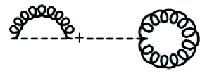
Figure 3: First order diagrams for $\Sigma\left(\mathbf{q}\right)$. The curly line represents the free correlator of flexural phonons, the dashed line corresponds to the 4-leg interaction vertex associated to $R_{ij,kl}\left(\mathbf{k}\right)$. The second diagram is $0$, since the $\mathbf{q}=0$ Fourier component of the transverse projector is integrated out during the in-plane modes Gaussian integration.

Recently it has been demonstrated how anharmonic effects in stiff membranes as graphene are highly suppressed by applying tension.Roldán et al. In this Appendix we show how the infrared cutoff $q_{c}$ of our (harmonic) theory depends on the applied strain. This is consistent with the sample to sample differences of order unity reported in recent measurements of electron mobilities in doped suspended monolayer graphene.Castro et al. (2010) As argued in Ref. Castro et al., 2010, comparing $q_{c}\approx 0.1\textrm{\AA}^{-1}$,Zakharchenko et al. (2010b) (the infrared cutoff for the harmonic theory in the absence of strain), and $q^{*}$ [the momentum scale associated to the presence of strain, defined by Eq. (55)] gives $u\sim 10^{-4}-10^{-3}$ as the strain involved in such kind of experiments. In order to estimate properly this number we have to know how $q_{c}$ is affected by strain. The discussion can be applied to both cases, monolayer or bilayer graphene.

In order to estimate anharmonic effects in the dispersion relation of FPs, since Eq. (1) is quadratic in the in-plane displacements we can integrate them out to obtain the effective free-energy for the out-of-plane degree of freedomNelson and Peliti (1987)

$$\mathcal{F}^{eff}=\frac{1}{2}\kappa\int dxdy\left(\nabla^{2}h\right)^{2}+\frac{1}{2}\int dxdyR_{ij,kl}\partial^{i}h\partial^{j}h\partial^{k}h\partial^{l}h,$$ (116)

where the four-point-coupling fourth-order tensor can be written as $R_{ij,kl}=\frac{K_{0}}{4}P_{ij}^{T}P_{kl}^{T}$, the operator $P_{ij}^{T}$ is the transverse projector $P_{ij}^{T}=\left(\nabla^{2}\right)^{-1}\varepsilon_{ik}\varepsilon_{jl}\partial^{k}\partial^{l}$, and $K_{0}=\frac{4\mu\left(\mu+\lambda\right)}{2\mu+\lambda}$. In order to include the effect of strain, we add to Eq. (116) the simplest term which breaks rotational symmetry

$$\frac{1}{2}\gamma\int dxdy\left(\nabla h\right)^{2},$$

where $\gamma$ is a sample-dependent coefficient with units of tension which can be related with the strain of the sample. This approach follows the spirit of the effective isotropic dispersion relation of FPs introduced in Eq. (8). If we add to Eq. (1) the most general term to first order in the derivatives of the displacement fields which breaks rotational symmetry and then we integrate out the in-plane degrees of freedom, we obtain a new two-point vertex whose contribution to the renormalization of the bending rigidity is weak and can be neglected.Roldán et al. . We are going to study the Fourier component of the height-height correlation function

$$G\left(\mathbf{q}\right)=\left\langle\left|h\left(\mathbf{q}\right)\right|^{2}\right\rangle=\frac{1}{Z}\int\mathcal{D}h\left(\mathbf{q}\right)\left|h\left(\mathbf{q}\right)\right|^{2}e^{S^{eff}\left[h\left(\mathbf{q}\right)\right]},$$

where obviously $Z=\int\mathcal{D}h\left(\mathbf{q}\right)e^{S^{eff}}$ is the partition function of the system, the effective action is nothing but $S^{eff}\left[h\left(\mathbf{q}\right)\right]=-\beta F^{eff}\left[h\left(\mathbf{q}\right)\right]$, and the Fourier transformed effective free energy reads

$$\mathcal{F}^{eff}\left[h\left(\mathbf{q}\right)\right]=\int\frac{d^{2}\mathbf{q}}{\left(2\pi\right)^{2}}\left(\frac{\kappa}{2}q^{4}+\frac{\gamma}{2}q^{2}\right)|h\left(\mathbf{q}\right)|^{2}+\frac{1}{2}\int\prod_{i=1}^{4}\frac{d^{2}\mathbf{q}_{i}}{\left(2\pi\right)^{8}}q_{1}^{i}q_{2}^{j}q_{3}^{k}q_{4}^{l}R_{ij,kl}\left(\mathbf{q}_{1}+\mathbf{q}_{2}\right)\delta^{(2)}\left(\mathbf{q}_{1}+\mathbf{q}_{2}+\mathbf{q}_{3}+\mathbf{q}_{4}\right),$$ (117)

where $R_{ij,kl}\left(\mathbf{k}\right)=\frac{K_{0}}{4}P_{ij}^{T}\left(\mathbf{k}\right)P_{ij}^{T}\left(\mathbf{k}\right)$, and the Fourier transformed transverse projector reads $P_{ij}^{T}\left(\mathbf{k}\right)=k^{-2}\varepsilon_{ik}\varepsilon_{jl}k^{k}k^{l}=\delta_{ij}-\frac{k_{i}k_{j}}{k^{2}}$. It is important to note that the $\mathbf{q}=0$ Fourier component of the transverse projector is integrated out during the Gaussian integration of the in-plane modes.Nelson and Peliti (1987) In the harmonic approximation and in the absence of strain ($\gamma=0$), the (free) correlator is given by

$$G^{(0)}\left(\mathbf{q}\right)=\frac{K_{B}T}{\kappa q^{4}}.$$ (118)

When we assume a quadratic dispersion relation we are taking this correlator as the proper one. This approximation is obviously affected by the presence of strain and anharmonic effects (also affected by strain), which renormalizes the bending rigidity $\kappa$. Then, we can write $G^{-1}\left(\mathbf{q}\right)\propto\kappa\left(\mathbf{q}\right)q^{4}$ and study the renormalization of $\kappa$ from the Dyson equation

$$G^{-1}\left(\mathbf{q}\right)=\left(G^{(0)}\left(\mathbf{q}\right)\right)^{-1}+\Sigma\left(\mathbf{q}\right),$$ (119)

where now the correlator in the harmonic theory, including the effect of strain, is given by

$$G^{(0)}\left(\mathbf{q}\right)=\frac{K_{B}T}{\kappa q^{4}+\gamma q^{2}}.$$ (120)

In order to estimate the anharmonic effects we compute the first order diagrams for self-energy, showed in Fig. 3. Only the first diagram gives a non-zero contribution

$$\Sigma^{(1)}\left(\mathbf{q}\right)=4\beta\int\frac{d^{2}\mathbf{k}}{\left(2\pi\right)^{2}}q^{i}q^{j}q^{k}q^{l}R_{ij,kl}\left(\mathbf{k}\right)G^{(0)}\left(\mathbf{q}-\mathbf{k}\right).$$ (121)

Replacing this result in equation Eq. (119) we obtain

$$\kappa\left(\mathbf{q}\right)=\kappa+\frac{\gamma}{q^{2}}+K_{B}TK_{0}\int\frac{d^{2}\mathbf{k}}{\left(2\pi\right)^{2}}\frac{\left(1-\frac{\left(\mathbf{q}\cdot\mathbf{k}\right)^{2}}{q^{2}k^{2}}\right)^{2}}{\kappa|\mathbf{q}-\mathbf{k}|^{4}+\gamma|\mathbf{q}-\mathbf{k}|^{2}}.$$ (122)

Follow the Ginzburg criterion,Fasolino et al. (2007) we estimate the cutoff of the theory nothing but comparing each correcting term of Eq. (122) with the bare value of $\kappa$. As we have already mentioned, there are two different cutoffs, the one given by strain in the harmonic approximation, and the other one associated to anharmonic effects. The first one is given by the second term of Eq. (122), and it is nothing but $q^{*}$,

$$q^{*}=\sqrt{\frac{\gamma}{\kappa}}.$$ (123)

Identifying this result with the momentum scale defined by Eq. (55), we deduce the relation between $\gamma$ and $u$: $\gamma=\left(\lambda+2\mu\right)u$.

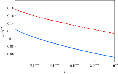
Figure 4: The infrared cutoff $q_{c}$ as a function of the applied strain $u$ for monolayer (in red dashed line) and bilayer graphene (in blue). In both cases $T=300$ K.

The cutoff of the harmonic theory is also affected by strain. Following the same criterion, its value comes from the solution to the equation

$$\kappa=\frac{K_{B}TK_{0}}{\left(2\pi\right)^{2}\kappa}\int_{0}^{2\pi}d\theta\int_{0}^{\infty}dk\frac{k\sin^{4}\left(\theta\right)}{\left(k^{2}+q^{2}-2kq\cos\left(\theta\right)\right)^{2}+\left(q^{*}\right)^{2}\left(k^{2}+q^{2}-2kq\cos\left(\theta\right)\right)}.$$ (124)

In the absence of strain, we have $q_{c}=\sqrt{\frac{3K_{B}TK_{0}}{16\pi\kappa^{2}}}$, which gives at $T=300$ K the value $q_{c}=0.178\textrm{\AA}^{-1}$ in the case of monolayer, and $q_{c}=0.126\textrm{\AA}^{-1}$ in the case of bilayer graphene. Its dependence on the applied strain is shown in Fig. 4. It is clear that $q_{c}$ decreases as the strain increases, so the unavoidable little strain present in real samples increases the validity of the harmonic approximation.

References

- Feldman et al. (2009) B. E. Feldman, J. Martin, and A. Yacoby, Nature Physics 5, 889 (2009).
- Zhang et al. (2009) Y. Zhang, T.-T. Tang, C. Girit, Z. Hao, M. C. Martin, A. Zettl, M. F. Crommie, Y. R. Shen, and F. Wang, Nature 459, 820 (2009).
- Bolotin et al. (2008) K. I. Bolotin, K. J. Sikes, Z. Jiang, G. Fudenberg, J. Hone, P. Kim, and H. L. Stormer, Solid State Commun. 146, 351 (2008).
- Du et al. (2008) X. Du, I. Skachko, A. Barker, and E. Y. Andrei, Nature Nanotech. 3, 491 (2008).
- Morozov et al. (2008) S. V. Morozov, K. S. Novoselov, M. I. Katsnelson, F. Schedin, D. Elias, J. A. Jaszczak, and A. K. Geim, Phys. Rev. Lett. 100, 016602 (2008).
- Castro et al. (2010) E. V. Castro, H. Ochoa, M. I. Katsnelson, R. V. Gorbachev, D. C. Elias, K. S. Novoselov, A. K. Geim, and F. Guinea, Phys. Rev. Lett. 105, 266601 (2010).
- Mariani and von Oppen (2010) E. Mariani and F. von Oppen, Phys. Rev. B 82, 195403 (2010).
- (8) H. Ochoa, E. V. Castro, M. I. Katsnelson, and F. Guinea, arXiv:1008.2523v1 [cond-mat.mtrl-sci].
- Bao et al. (2009) W. Bao, F. Miao, Z. Chen, H. Zhang, W. Jang, C. Dames, and C. N. Lau, Nature Nanotech. 4, 562 (2009).
- Chen et al. (2009) C. Chen, S. Rosenblatt, K. I. Bolotin, W. Kalb, P. Kim, I. Kymissis, H. L. Stormer, T. F. Heinz, and J. Hone, Nature Nanotech. (2009), published online: 20 September 2009.
- Castro Neto et al. (2009) A. H. Castro Neto, F. Guinea, N. M. R. Peres, K. S. Novoselov, and A. K. Geim, Rev. Mod. Phys. 81, 109 (2009).
- Zakharchenko et al. (2009) K. V. Zakharchenko, M. I. Katsnelson, and A. Fasolino, Phys. Rev. Lett. 102, 046808 (2009).
- Landau and Lifshitz (1970) L. D. Landau and E. M. Lifshitz, Theory of Elasticity (Pergamon Press, Oxford, 1970), 2nd ed.
- Nelson et al. (2004) D. Nelson, T. Piran, and S. Weinberg, eds., Statistical Mechanics of Membranes and Surfaces (World Scientific, New Jersey, 2004), 2nd ed.
- Kudin et al. (2001) K. N. Kudin, G. E. Scuseria, and B. I. Yakobson, Phys. Rev. B 64, 235406 (2001).
- Lee et al. (2008) C. Lee, X. Wei, J. W. Kysar, and J. Hone, Science 321, 385 (2008).
- Zakharchenko et al. (2010a) K. Zakharchenko, J. Los, M. I. Katsnelson, and A. Fasolino, Phys. Rev. B 81, 235439 (2010a).
- Mariani and von Oppen (2008) E. Mariani and F. von Oppen, Phys. Rev. Lett. 100, 076801 (2008).
- Fogler et al. (2008) M. M. Fogler, F. Guinea, and M. I. Katsnelson, Phys. Rev. Lett. 101, 226804 (2008).
- Suzuura and Ando (2002) H. Suzuura and T. Ando, Phys. Rev. B 65, 235412 (2002).
- Choi et al. (2010) S.-M. Choi, S.-H. Jhi, and Y.-W. Son, Phys. Rev. B 81, 081407(R) (2010).
- Morozov et al. (2006) S. V. Morozov, K. S. Novoselov, M. I. Katsnelson, F. Schedin, L. A. Ponomarenko, D. Jiang, and A. K. Geim, Phys. Rev. Lett. 97, 016801 (2006).
- Katsnelson and Novoselov (2007) M. Katsnelson and K. Novoselov, Solid State Commun. 143, 3 (2007).
- Katsnelson and Geim (2008) M. I. Katsnelson and A. K. Geim, Phil. Trans. R. Soc. A 366, 195 (2008).
- Guinea et al. (2008) F. Guinea, B. Horovitz, and P. L. Doussal, Phys. Rev. B 77, 205421 (2008).
- Altland and Simons (2006) A. Altland and B. Simons, Condensed Matter Field Theory (Cambridge University Press, Cambridge, 2006).
- Auslender and Katsnelson (2007) M. Auslender and M. I. Katsnelson, Phys. Rev. B 76, 235425 (2007).
- Cappelluti and Benfatto (2009) E. Cappelluti and L. Benfatto, Phys. Rev. B 79, 035419 (2009).
- Ziman (1960) J. M. Ziman, Electrons and Phonons: the theory of transport phenomena in solids (Oxford Univesity Press, London, 1960).
- (30) The fact that scattering is elastic and the Fermi surface isotropic makes unimportant factors depending only on , the absolute value of momentum.
- Irkhin and Katsnelson (2002) V. Y. Irkhin and M. I. Katsnelson, Eur. Phys. J. B 30, 481 (2002).
- (32) H. Min, E. H. Hwang, and S. D. Sarma, arXiv:1011.0741v1 [cond-mat.mtrl-sci].
- Hwang and Sarma (2008) E. H. Hwang and S. D. Sarma, Phys. Rev. B 77, 115449 (2008).
- Stauber et al. (2007) T. Stauber, N. M. R. Peres, and F. Guinea, Phys. Rev. B 76, 205423 (2007).
- Chen et al. (2008) J. H. Chen, C. Jang, S. Xiao, M. Ishigami, and M. S. Fuhrer, Nature Nanotech. 3, 206 (2008).
- Efetov and Kim (2010) D. K. Efetov and P. Kim, Phys. Rev. Lett. 105, 256805 (2010).
- Zakharchenko et al. (2010b) K. V. Zakharchenko, R. Roldan, A. Fasolino, and M. I. Katsnelson, Phys. Rev. B 82, 125435 (2010b).
- (38) R. Roldán, A. Fasolino, K. V. Zakharchenko, and M. I. Katsnelson, arXiv:1101.6026v1 [cond-mat.mtrl-sci].
- Landau and Lifshitz (1981) L. D. Landau and E. M. Lifshitz, Physical Kinetics, vol. 5 (Pergamon, 1981), 1st ed.
- Nelson and Peliti (1987) D. R. Nelson and L. Peliti, J. Physique 48, 1085 (1987).
- Fasolino et al. (2007) A. Fasolino, J. H. Los, and M. I. Katsnelson, Nat. Mater. 6, 858 (2007).