Rare $B$ Decays Potential at Super$B$

Abstract:

We present a short overview of the most important rare $B$ decay analyses which will be performed using $75~{}{\rm ab}^{-1}$ dataset which is expected to be provided by Super$B$ Factory within five years from its starting date.

1 Motivation for Super$B$ Factory

1.1 Why Rare Decays?

There are two major ways to discover physics beyond the Standard Model (SM). The first one is to directly produce non-SM particles in collisions and detect their decay products, the second one is to observe the effects of these particles on the decay rates of the rare decays of the SM bound states. The former way requires high energy, the latter – high statistics. The discovery of the $c$-quark proved the validity of both ways: initially heavy $c$-quark was introduced to bring the theoretically calculated decay rate of the rare decay of light meson $K_{L}\to\mu^{+}\mu^{-}$ into agreement with the experiment [1], and only later it was found in direct production and decay of the $J/\psi$ bound state [2]. Following this historical lesson, one can look for the effects of extremely heavy non-SM particles in the decays of much lighter $B$-mesons.

1.2 Why Rare $B$ Decays?

The decays of the heavy $b$-quark involve all the lighter quarks, therefore one has more chances to find non-SM effects. There are many processes sensitive to these effects, including $B^{0}$-$\overline{B^{0}}$ mixing, penguin decays $b\to s\gamma$, $b\to s\ell^{+}\ell^{-}$ and $b\to s\nu\bar{\nu}$, transitions $b\to sq\bar{q}$, $b\to dq\bar{q}$, and annihilations $b\bar{q}\to\ell^{+}\ell^{-}$ and $b\bar{q}\to\ell\nu$. A few examples of possible New Physics (NP) contributions to $b\to s\nu\bar{\nu}$ decay are shown in the diagrams in Fig. 1.

Figure 1: Possible NP contributions to $b\to s\nu\bar{\nu}$ decay.

1.3 Why Super(B)-Flavor Factory?

The projected Super$B$ factory [3] is a linear $e^{+}e^{-}$ collider intended to deliver instantaneous luminosity of ${\cal L}=10^{36}~{}{\rm cm}^{-2}~{}{\rm s}^{-1}$ at the same center-of-mass energy as the current $B$-factories: the mass of $\Upsilon(4S)$. In five years ($1.5\times 10^{8}~{}{\rm s}$) of running with estimated $\sim\!50\%$ downtime Super$B$ is expected to collect $\sim\!75~{}{\rm ab}^{-1}$ of data. This is two orders of magnitude larger than the currently available datasets collected by BABAR ($0.53~{}{\rm ab}^{-1}$) and Belle ($0.95~{}{\rm ab}^{-1}$). This humongous dataset will drastically improve our chances to find the New Physics effects in rare $B$ decays. And if (when) LHC finds the New Physics before the start of Super$B$, the flavor content of this New Physics will still have to determined, and Super$B$ will be playing major role in this.

2 Experimental Technique

Fully-reconstructible rare $B$ decays (such as $B_{(s)}\to\mu\mu$ or $B_{(s)}\to K^{(*)}\mu\mu$) can be analysed at both hadronic machines (LHC, Tevatron) and Super$B$. But those rare $B$ decays which contain one or more neutrinos in the final state can only be investigated in clean $e^{+}e^{-}$ environment. The corresponding data analyses at Super$B$ will be exploiting the same recoil technique which has been extensively used in $B$-factories: full or partial reconstruction of one $B$-meson (the tag $B$) and ascribing all the remaining objects to the second $B$-meson (the signal $B$) – see Fig. 2.

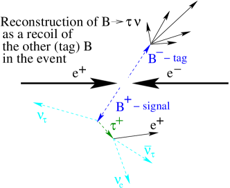
Figure 2: Rare $B$ decays with one or more neutrinos in the final state can only be done in $e^{+}e^{-}$ machines.

The tag $B$ meson can be reconstructed in two ways. In the first one it is fully-reconstructed in the decay into pure hadronic final state. This technique gives better kinematic constraint of the $B$ meson but has a lower reconstruction efficiency ($\sim\!0.4\%$). In the second way, the tag $B$ meson is partially reconstructed in the decay into semileptonic final state with missing neutrino. Obviously, in this case the kinematic constraint is much worse, but the reconstruction efficiency is higher ($\sim\!2.0\%$).

A very important quantity here is so-called $E_{extra}$ – the sum of all the energy depositions in the Electromagnetic Calorimeter (EMC) not associated with any physics objects. In a well-reconstructed event $E_{extra}$ must be of the order of 200-300 ${\rm MeV}/c^{2}$ (calorimeter noise), but in the events where we actually miss a particle it can be larger. Super$B$ will have an additional backward end-cap EMC with respect to BABAR EMC configuration, to diminish the amount of lost particles.

3 Rare $B$ Decays

3.1 $b\to s\nu\bar{\nu}$

Theoretically, it is better to measure inclusive decay rate $B\to X_{s}\nu\bar{\nu}$, but such analysis would be challenging from experimental point of view. For this reason we are going to measure the rates of the exclusive decays $B_{u}\to K\nu\bar{\nu}$ and $B_{d}\to K^{*0}\nu\bar{\nu}$. The latter decays has another observable – longitudinal polarization $\langle F_{L}\rangle$ properly averaged over the neutrinos’ invariant mass [4] – which is easy to calculate. The current limits of the decay rates are about an order of magnitude larger than SM predictions (Tab. 1).

Observable	SM prediction	Experiment
$\mathcal{B}(B^{0}\to K^{*0}\nu\bar{\nu})$	$(6.8^{+1.0}_{-1.1})\times 10^{-6}$ [4]	$<80\times 10^{-6}$ [5]
$\mathcal{B}(B^{+}\to K^{+}\nu\bar{\nu})$	$(3.6\pm 0.5)\times 10^{-6}$ [6]	$<14\times 10^{-6}$ [7]
$\mathcal{B}(\bar{B}\to X_{s}\nu\bar{\nu})$	$(2.7\pm 0.2)\times 10^{-5}$ [4]	$<64\times 10^{-5}$ [8]
$\langle F_{L}(B^{0}\to K^{*0}\nu\bar{\nu})\rangle$	$0.54\pm 0.01$ [4]	–

Table 1: SM predictions and experimental 90% C.L. upper bounds for the four $b\to s\nu\bar{\nu}$ observables.

It is possible to parametrize the deviations of all the branching fractions from their SM values in terms of only two phenomenological parameters $\epsilon$ and $\eta$ which are respectively equal to 1 and 0 in SM:

$$R(B\to K^{*}\nu\bar{\nu}) = (1+1.31\,\eta)\epsilon^{2},$$ (1)

$$R(B\to K\nu\bar{\nu}) = (1-2\,\eta)\epsilon^{2},$$ (2)

$$R(\bar{B}\to X_{s}\nu\bar{\nu}) = (1+0.09\,\eta)\epsilon^{2},$$ (3)

$$\langle F_{L}\rangle/\langle F_{L}\rangle_{\rm SM} = \frac{(1+2\,\eta)}{(1+1.31\,\eta)},$$ (4)

where $R(X)=\mathcal{B}(X)/\mathcal{B}(X)_{\rm SM}$. Notice that $\langle F_{L}\rangle$ does not depend on $\epsilon$. An experimental observation of such a dependence would be a sign for the existence of the right-handed currents. The plots in Fig. 3 (Refs. [9, 10]) demonstrate current theoretical and experimental constraints in $\epsilon$-$\eta$ plane.

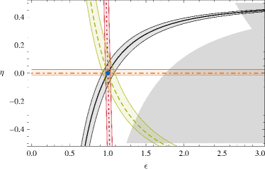
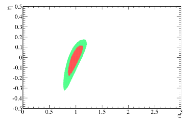
Figure 3: Left: Theoretical (4 colored bands) and 90% C.L. experimental (grey area) constraints on $\epsilon$ and $\eta$. The green band (dashed line) shows the constraint from $\mathcal{B}(B\to K^{*}\nu\bar{\nu})$, the black band (solid line) – $\mathcal{B}(B\to K\nu\bar{\nu})$, the red band (dotted line) – $\mathcal{B}(B\to X_{s}\nu\bar{\nu})$, and the orange band (dot-dashed line) – $\langle F_{L}\rangle$. Right: Expected 68% C.L. (green) and 95% C.L. (red) constraints on $\epsilon$ and $\eta$ from $75~{}{\rm ab}^{-1}$ at Super$B$.

3.2 $B\to\ell\nu$

This annihilation proceeds via charged current and is sensitive to the charged Higgs, especially for the large values of $\tan\beta$. The Two Higgs Double Model (2HDM) yields

$$\frac{\mathcal{B}(B\to\ell\nu_{\ell})_{2HDM}}{\mathcal{B}(B\to\ell\nu_{\ell})_{SM}}=\left(1-\frac{m_{B}^{2}\tan^{2}\beta}{m^{2}_{H^{\pm}}}\right)^{2}.$$

The $\mathcal{B}(B\to\tau\nu_{\tau})$ is within the reach of current $B$-factories and has already been measured by BABAR [11] and Belle [12] but Super$B$ is expected to significantly improve the precision, as well as measure the $\mathcal{B}(B\to\mu\nu_{\mu})$. The plots in Fig. 4 demonstrate the excluded regions for $\tan\beta$ and the mass of the charged Higgs for the currently available total dataset ($2~{}{\rm ab}^{-1}$) and for the expected dataset from Super$B$ ($75~{}{\rm ab}^{-1}$) for both $B\to\tau\nu_{\tau}$ and $B\to\mu\nu_{\mu}$ analyses together. With further increase of the dataset beyond $75~{}{\rm ab}^{-1}$ the uncertainty on $\mathcal{B}(B\to\tau\nu_{\tau})$ becomes systematics-dominated while $\mathcal{B}(B\to\mu\nu_{\mu})$ keeps scaling with statistics.

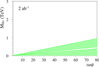
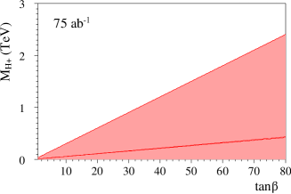
Figure 4: Excluded regions for the currently available total dataset ($2~{}{\rm ab}^{-1}$) and for the expected dataset from Super$B$ ($75~{}{\rm ab}^{-1}$) for both $B\to\tau\nu_{\tau}$ and $B\to\mu\nu_{\mu}$ analyses together.

3.3 $B\to\ell\nu\gamma,B_{(s)}\to\ell\ell\gamma,B_{(s)}\to\gamma\gamma$

The branching fractions of these radiative decays have no hadronic uncertainties and no helicity suppression (due to the presence of the photon). The SM predictions together with current experimental limits on the branching fractions are given in Tab. 2. Super$B$ will be able to improve the existing measurements on $B_{(s)}$ decays and, possibly, setup a limit on $B_{s}\to\ell\ell\gamma$ decay.

Process	SM Branching Fraction	Experiment 90% C.L.
$B\to\ell\nu\gamma$	$\mathcal{O}(10^{-6})$ [13]	$1.56\times 10^{-5}$ [14]
$B\to\ell\ell\gamma$	$\mathcal{O}(10^{-10})$ [13]	$\sim\!10^{-7}$ [14]
$B_{s}\to\ell\ell\gamma$	$\mathcal{O}(10^{-9})$ [13]	–
$B\to\gamma\gamma$	$\mathcal{O}(10^{-8})$ [13]	$6.2\times 10^{-7}$ [14]
$B_{s}\to\gamma\gamma$	$(2$-$8)\times 10^{-7}$ [15]	$8.7\times 10^{-6}$ [14]

Table 2: SM predictions and current experimental limits on the radiative branching fractions.

3.4 $b\to s\gamma$

Similar to $b\to s\nu$, this decay is sensitive to charged Higgs in 2HDM-II model. The bound on the charged Higgs mass from the left plot in Fig. 5 ($M_{H^{+}}=295~{}{\rm GeV}/c^{2}$ at $95\%~{}C.L.$) is the strongest available one [16]. Another application of $b\to s\gamma$ decay – extra dimensions. The bound on the inverse compactification radius $1/R$ at $95\%$ C.L. in the minimal Universal Extra Dimension model (mUED) shown in the right plot Fig. 5 from Ref. [17]. Super$B$ will definitely improve both plots with the expected systematic uncertainty (3%) dominating over the statistical one. It is also worth mentioning here that in producing these plots the $B$-factories used only more efficient semileptonic tag $B$, while Super$B$ will be able to use more kinematically-constrained hadronic tag $B$ as well.

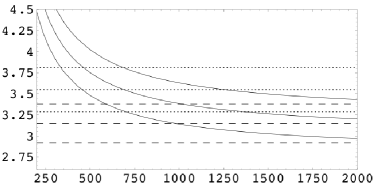
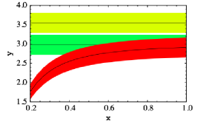
Figure 5: Left: ${\cal B}(\bar{B}\to X_{s}\gamma)~{}[10^{-4}]$ as a function of the charged Higgs boson mass $M_{H^{+}}~{}[GeV/c^{2}]$ in the 2HDM II for $\tan\beta=2$ (solid lines). The dashed lines represent SM (central value plus-minus uncertainty), the dotted lines – experiment. Right: $y\equiv{\mathcal{B}}(\bar{B}\to X_{s}\gamma)~{}[10^{-4}]$ as a function of inverse compactification radius $x\equiv 1/R~{}[{\rm TeV}]$ of mUED. The red (dark gray) band corresponds to the LO mUED result. The yellow (light gray) band – 68% C.L. experimental range, the green (medium gray) band – SM.

3.5 $b\to s\ell\ell$

This rare decay is sensitive to the right-handed currents and multitude of different types of NP. There are two approaches to this decay: reconstruction of all the exclusive decay modes and inclusive recoil analysis with two leptons in the recoil. The first method is quite complicated experimentally and not so clean from the theoretical point of view. The second method is better theoretically, but has a disadvantage of low $B$-tagging efficiency and admixture of $b\to d\ell\ell$. Therefore, the third approach is usually used – exclusive reconstruction of only two modes: $B_{u}\to K\ell\ell$ and $B_{d}\to K^{*0}\ell\ell$. By simple extrapolation we expect an order of magnitude better statistical uncertainty and a factor of two better systematic uncertainty in $75~{}{\rm ab}^{-1}$ data sample in Super$B$ than in the corresponding BABAR analyses.

3.6 Super$B$ Performance at $75~{}{\rm ab}^{-1}$

Finally, the uncertainties on the branching fractions of the most important rare $B$ decays projected to $75~{}{\rm ab}^{-1}$ dataset expected at Super$B$ are presented in Tab. 3 (Refs. [18, 19, 20, 21]). As we can see, a significant improvement or a completely new measurement is expected for all the channels.

Mode	Sensitivity
	Current	Expected ($75\ {\rm ab}^{-1}$)
${\cal B}(B\to X_{s}\gamma)$	7%	3%
${\cal B}(B^{+}\to\tau^{+}\nu)$	30%	3–4%
${\cal B}(B^{+}\to\mu^{+}\nu)$	not measured	5–6%
${\cal B}(B\to X_{s}\ell^{+}\ell^{-})$	23%	4–6%
${\cal B}(B\to K\nu\overline{\nu})$	not measured	16–20%

Table 3: The uncertainties on the branching fractions of the most important rare $B$ decays projected to $75~{}{\rm ab}^{-1}$ dataset expected at Super$B$.

4 Summary

In conclusion, the Super$B$ Factory will be able to either spot New Physics in the rare $B$ decays or to investigate flavor content of the New Physics found at LHC, within only a few years after its start!

5 Acknowledgments

The author would like to thank the conference organizers for the opportunity to present this poster.

References

- [1] S. L. Glashow, J. Iliopoulos, and L. Maiani, Phys. Rev. D2, 1285 (1970)
- [2] J. Aubert et al., Phys. Rev. Lett. 33, 1402 (1974); J. E. Augustin et al., Phys. Rev. Lett. 33, 1406 (1974)
- [3] E. Grauges et al. [SuperB Collaboration], arXiv:1007.4241
- [4] W. Altmannshofer, A. J. Buras, D. M. Straub, and M. Wick, JHEP 04, 022 (2009), arXiv:0902.0160
- [5] B. Aubert et al. [BABAR Collaboration], Phys. Rev. D78, 072007 (2008), arXiv:0808.1338
- [6] M. Bartsch, M. Beylich, G. Buchalla, and D. N. Gao, JHEP 11, 011 (2009), arXiv:0909.1512
- [7] K. F. Chen et al. [BELLE Collaboration], Phys. Rev. Lett. 99, 221802 (2007), arXiv:0707.0138
- [8] R. Barate et al. [ALEPH Collaboration], Eur. Phys. J. C19, 213 (2001), arXiv:hep-ex/0010022
- [9] A. Bevan et al. [Super Collaboration], arXiv:1008.1541
- [10] A. Bevan, arXiv:hep-ex/0611031
- [11] P. del Amo Sanchez et al., [BABAR Collaboration], arXiv:1008.0104; B. Aubert et al. [BABAR Collaboration], arXiv:0708.2260; B. Aubert et al. [BABAR Collaboration], arXiv:hep-ex/0304030; B. Aubert et al. [BABAR Collaboration], arXiv:hep-ex/0608019; B. Aubert et al. [BABAR Collaboration], arXiv:0705.1820; B. Aubert et al. [BABAR Collaboration], arXiv:hep-ex/0408091
- [12] K. Abe et al. [Belle Collaboration], Phys. Rev. Lett. 97, 251802 (2006); K. Abe et al. [Belle Collaboration], arXiv:1006.4201; K. Abe et al. [Belle Collaboration], arXiv:hep-ex/0507034; K. Abe et al. [Belle Collaboration], arXiv:hep-ex/0408144
- [13] D. Hitlin et al., arXiv:0810.1312
- [14] K. Nakamura et al. [Particle Data Group], J. Phys. G 37, 075021 (2010)
- [15] L. Reina, G. Ricciardi, and A. Soni, Phys. Rev. D56, 5805 (1997), arXiv:hep-ph/9706253
- [16] M. Misiak et al., Phys. Rev. Lett. 98, 022002 (2007), arXiv:hep-ph/0609232
- [17] U. Haisch and A. Weiler, Phys. Rev. D76, 034014 (2007), arXiv:hep-ph/0703064
- [18] M. Rama, arXiv:0909.1239
- [19] M. Bona et al., arXiv:0709.0451
- [20] T. Browder et al., JHEP 0802 (2008) 110, arXiv:0710.3799
- [21] T. Browder et al., arXiv:0802.3201