Meridional circulation in turbulent protoplanetary disks

Abstract

Context. Based on the viscous disk theory, a number of recent studies have suggested there is large scale meridional circulation in protoplanetary disks. Such a flow could account for the presence of crystalline silicates, including calcium– and aluminum–rich inclusions (CAIs), at large distances from the sun.

Aims. This paper aims at examining whether such large–scale flows exist in turbulent protoplanetary disks.

Methods. High–resolution global hydrodynamical and magnetohydrodynamical (MHD) numerical simulations of turbulent protoplanetary disks were used to infer the properties of the flow in such disks.

Results. By performing hydrodynamic simulations using explicit viscosity, we demonstrate that our numerical setup does not suffer from any numerical artifact. The aforementioned meridional circulation is easily recovered in viscous and laminar disks and is quickly established. In MHD simulations, the magnetorotational instability drives turbulence in the disks. Averaging out the turbulent fluctuations on a long timescale, the results fail to show any large–scale meridional circulation. A detailed analysis of the simulations show that this lack of meridional circulation is due to the turbulent stress tensor having a vertical profile different from the viscous stress tensor. A simple model is provided that successfully accounts for the structure of the flow in the bulk of the disk. In addition to those results, possible deviations from standard vertically averaged $\alpha$ disk models are suggested by the simulations and should be the focus of future work.

Conclusions. Global MHD numerical simulations of fully ionized and turbulent protoplanetary disks are not consistent with the existence of a large–scale meridional flow. As a consequence, the presence of crystalline silicates at large distance for the central star cannot be accounted for by that process as suggested by recent models based on viscous disk theory.

1 Introduction

In the past few years, more and more evidence has accumulated that suggests there are crystalline solid particles in the outer regions of protoplanetary disks. Spitzer observations in the $5$–$35$ $\mu$m spectral range have revealed crystalline signatures in a large fraction of T–Tauri stars (Bouwman et al. 2008; Olofsson et al. 2009; Sargent et al. 2009). Comets, which are believed to form far away from the Sun, are also known to show high crystallinity values (Crovisier et al. 1997; Wooden et al. 1999, 2007). This has recently been independently confirmed by the returned samples of the Stardust mission (Brownlee et al. 2006; Zolensky et al. 2006). Meteoritic records also indicate that calcium– and aluminum–rich inclusions (CAIs) are a common component of chondrites collected from parent bodies thought to originate in the main asteroid belt. CAIs, as well as the crystalline silicates observed by the Spitzer telescope, are believed to have formed in the inner parts of protoplanetary disks ($R\leq 1$ AU) where temperatures are in excess of $\sim$$1000$ K as required for their formation from amorphous silicates. This general trend of finding crystalline silicates at large distances from the central star requires a mechanism able to transport them from the disk’s inner parts to their outer regions.

Several processes have been suggested to account for such transport. Shu et al. (1996, 2001) have invoked the action of powerful winds from the young stars, the so–called X–wind model (see also Hu 2010). Many authors have, on the other hand, relied on processes operating within the bulk of the disk itself. Indeed, the flow in accretion disks is believed to be turbulent in order for angular momentum to be efficiently transported outward. The turbulent nature of the flow results in an efficient diffusion of small solids in the disk, potentially transporting some of them to large heliocentric distances. Using the standard 1D (i.e. vertically integrated) $\alpha$ disk model (Shakura & Sunyaev 1973; Lynden-Bell & Pringle 1974) as a theoretical basis to model the effect of the turbulence, Gail (2001) and Bockelée-Morvan et al. (2002) have quantified the resulting concentration of crystalline silicates in the outer parts of protoplanetary disks. The conclusion is that turbulence alone appears unable to transport enough solid material out to large distances because the inward flow associated with mass accretion onto the central object dominates over a long time and reduces its effect. As a remedy, several papers have invoked the existence of a large–scale meridional flow in protoplanetary disks. Such a meridional circulation naturally arises out of viscous disk models that extend the standard $\alpha$ disk model to two dimensions, the radial position $R$ and distance to the midplane Z (Urpin 1984; Siemiginowska 1988; Kley & Lin 1992; Rozyczka et al. 1994; Regev & Gitelman 2002; Takeuchi & Lin 2002). In these models, the radial velocity is positive in the disk’s equatorial plane while gas accretion proceeds through the disk surfaces. This outwardly directed mass flux advectively transports solids sedimented in the disk equatorial plane out to large distances and thus circumvents the limiting effect of mass accretion mentioned above. Several models based on this idea have been developed in the last few years (Takeuchi & Lin 2002; Keller & Gail 2004; Tscharnuter & Gail 2007; Ciesla 2007, 2009; Hughes & Armitage 2010). They have indeed been able to successfully reproduce the amount of crystalline solids found in outer protoplanetary disks.

However, all of these models rely on the $\alpha$ prescription, a large–scale model for the turbulence. While the nature of the turbulence in protoplanetary disks is still somewhat debated, it is most likely magnetohydrodynamical (MHD) in nature and driven by the magnetorotational instability (MRI, Balbus & Hawley 1991, 1998). Thanks to the large increase in computational resources, it is now possible to perform global numerical simulations of protoplanetary disks (Papaloizou & Nelson 2003; Fromang & Nelson 2006; Lyra et al. 2008) and to apply such simulations to a variety of issues related to planet formation, including dust dynamics (Fromang & Nelson 2005; Lyra et al. 2008; Fromang & Nelson 2009), planetesimals evolution (Nelson 2005; Nelson & Gressel 2010), dead–zone properties (Dzyurkevich et al. 2010), and planet–disk interaction (Nelson & Papaloizou 2003; Papaloizou et al. 2004; Nelson & Papaloizou 2004; Winters et al. 2003). Using such simulations, the nature of the large–scale flow can be investigated from first principles without having to rely on ad hoc modeling of the turbulence. It is the purpose of the present paper to develop such dedicated numerical simulations in order to validate the models of meridional circulation presented above that are used to explain the presence of crystalline solids at large distances from the central objects in protoplanetary disks.

The plan of the paper is as follows. In section 2, we describe the properties of meridional circulation as it can be derived from 2D viscous disk theory. Section 3 presents a set of numerical simulations of protoplanetary disks and analyzes the properties of the large–scale flow. In section 4, an additional series of purely hydrodynamical simulations are used to assess the influence of the numerical setup and algorithm on meridional circulation. Finally, in section 5, the results are discussed using a simple model and their consequences for crystalline silicates radial mixing are highlighted.

2 Large scale flow in protoplanetary disks

In this section, we seek to derive the equations that govern the large–scale radial flow in protoplanetary disks. To do so, we consider an axisymmetric disk and derive its global structure. The large–scale gas flow is determined by the mechanism governing angular momentum transport. Two cases will be considered. We first examine the case of viscous disk models in section 2.3 and adopt the standard $\alpha$ prescription for the kinematic viscosity. The analysis we present largely follows the equations derived, for example, by Takeuchi & Lin (2002) to which the reader is referred for further details. Since the flow in protoplanetary disk is most likely turbulent, we also write in section 2.4 the equations that govern angular momentum transport in such disks, highlighting the similarities and differences with viscous disk models.

2.1 Definitions

Unless otherwise stated, we consider in this paper a cylindrical coordinate system $(R,\phi,Z)$ with unit vectors $(\mbox{\boldmath{$e_{R}$}},\mbox{\boldmath{$e_{\phi}$}},\mbox{\boldmath{$e_{Z}$}})$. The disk model is fully specified once the equation of state (EOS), midplane density, and viscosity are chosen. For the former, we used a locally isothermal EOS: the sound speed is time independent and given as a function of the cylindrical radius $R$ by the power law,

$$c_{s}^{2}=c_{0}^{2}\left(\frac{R}{R_{0}}\right)^{q}\,,$$ (1)

where $c_{0}$ is the sound speed at the fidutial radius $R=R_{0}$. The disk midplane density $\rho_{mid}$ is similarly given by

$$\rho_{mid}=\rho_{0}\left(\frac{R}{R_{0}}\right)^{p}\,,$$ (2)

in which $\rho_{0}$ stands for the gas density at $R=R_{0}$.

2.2 Density and angular velocity

The first step is to derive the spatial distribution of gas density and angular velocity. They are given by the equations of force balance in the radial and vertical direction:

$$R\Omega^{2}-\frac{GMR}{(R^{2}+Z^{2})^{3/2}}-\frac{1}{\rho}\frac{\partial P}{\partial R} = 0\,,$$ (3)

$$-\frac{GMZ}{(R^{2}+Z^{2})^{3/2}}-\frac{1}{\rho}\frac{\partial P}{\partial Z} = 0\,.$$ (4)

The second equation gives the vertical profile for the density:

$$\rho(R,Z)=\rho_{0}\left(\frac{R}{R_{0}}\right)^{p}\exp\left(\frac{GM}{c_{s}^{2}}\left[\frac{1}{\sqrt{R^{2}+Z^{2}}}-\frac{1}{R}\right]\right)\,,$$ (5)

where Eq. (2) has been used to write the disk midplane density. Upon expanding Eq. (5) to the second order in $Z/R$, one recovers the standard Gaussian vertical profile

$$\rho(R,Z)=\rho_{0}\left(\frac{R}{R_{0}}\right)^{p}\exp\left(-\frac{Z^{2}}{2H^{2}}\right)\,,$$ (6)

where $H=c_{s}/\Omega_{K}$ is the disk scale height, which is the ratio of the sound speed to the Keplerian angular velocity $\Omega_{K}=\sqrt{GM/R^{3}}$. In this last definition, $G$ and $M$ stand for the gravitational constant and the central stellar mass, respectively . With the definition of $c_{s}$ given in section 2.1, $H$ can be expressed as

$$H=H_{0}\left(\frac{R}{R_{0}}\right)^{(q+3)/2}\,,$$ (7)

where $H_{0}=c_{0}/\sqrt{GM/R_{0}^{3}}$ is the disk scale height at $R=R_{0}$. Finally, Eq. (3), along with the expression for the gas density, gives the spatial variations of $\Omega$:

$$\Omega = \Omega_{K}\left[(1+q)-\frac{qR}{\sqrt{R^{2}+Z^{2}}}+(p+q)\left(\frac{H}{R}\right)^{2}\right]^{1/2}$$ (8)

$$= \Omega_{K}\left[1+\frac{1}{2}\left(\frac{H}{R}\right)^{2}\left(p+q+\frac{q}{2}\frac{Z^{2}}{H^{2}}\right)\right]\,.$$

where the last equality results from a second–order expansion in $Z/R$.

These expressions for the density and the angular velocity do not depend on the viscous or turbulent nature of the flow. In particular, they are expected to hold in turbulent protoplanetary disks provided turbulent fluctuations are properly averaged out on long timescales, as well as in viscous accretion disks regardless of the form of the viscous stress tensor. We show in section 3.2.1 that this is indeed the case.

2.3 Angular momentum conservation in viscous disks

A widespread and convenient way of modeling the effect of disk turbulence is to solve the hydrodynamic equations adding a nonzero kinematic viscosity. Since the early $1970$’s, this has led to the development of $\alpha$ disk models in which the kinematic viscosity is assumed to be of the form (Shakura & Sunyaev 1973; Lynden-Bell & Pringle 1974)

$$\nu=\alpha c_{s}H\,.$$ (9)

In this section, we examine the consequences of such a prescription on the disk’s large–scale radial flow. Angular momentum conservation writes in this case as

$$\rho\left(v_{R}\frac{\partial}{\partial R}+v_{Z}\frac{\partial}{\partial Z}\right)(R^{2}\Omega)$$ (10)

$$\hskip 42.67912pt=\frac{\partial}{\partial R}\left(R^{2}T_{R\phi}^{visc}\right)+\frac{\partial}{\partial Z}\left(R^{2}T_{Z\phi}^{visc}\right)\,,$$

where the viscous stress components $T_{R\phi}^{visc}$ and $T_{Z\phi}^{visc}$ are given by

$$T_{R\phi}^{visc} = \rho\nu R\frac{\partial\Omega}{\partial R}$$ (11)

$$T_{Z\phi}^{visc} = \rho\nu R\frac{\partial\Omega}{\partial Z}\,.$$ (12)

In addition, we have the orderings $v_{Z}$ $\sim$ $(H/R)v_{R}$ and $\partial/\partial Z$ $\sim$ $(H/R)\partial/\partial R$. Thus, in Eq. (10), the term $v_{Z}\partial/\partial Z$ is a factor $(H/R)^{2}$ smaller than the term $v_{R}\partial/\partial R$ and can be safely neglected in thin disks for which $H$$\ll$$R$ (Takeuchi & Lin 2002). This gives

$$R\rho v_{R}\frac{\partial R^{2}\Omega}{\partial R}=\frac{\partial}{\partial R}\left(R^{3}\rho\nu\frac{\partial\Omega}{\partial R}\right)+\frac{\partial}{\partial Z}\left(R^{3}\rho\nu\frac{\partial\Omega}{\partial Z}\right)\,.$$ (13)

At this point, an expansion to the second order in $(Z/R)$ is performed in order to proceed further in the analysis. After some manipulations and using Eq. (9) for the kinematic viscosity, the radial velocity can be expressed as (Takeuchi & Lin 2002)

$$\frac{v_{R}}{c_{0}}=-\alpha\left(\frac{H_{0}}{R_{0}}\right)\left(\frac{R}{R_{0}}\right)^{q+1/2}$$ (14)

$$\hskip 56.9055pt\left[3p+2q+6+\frac{5q+9}{2}\left(\frac{Z}{H}\right)^{2}\right]\,.$$

In the disk midplane, the radial velocity is thus positive whenever $3p+2q+6<0$, which is readily obtained for standard disks parameters. For example, typical values generally considered in numerical simulations are $q=-1$ and $p=-3/2$ (Fromang & Nelson 2006, 2009; Lyra et al. 2009; Dzyurkevich et al. 2010), and they correspond to outward midplane velocities. For these typical parameters, the second term appearing in front of the $Z$ dependence is positive. This indicates that the flow direction reverses in the disk’s upper layers to become negative. Overall, this flow pattern produces a meridional circulation in the disk in which gas flows outward in the disk midplane and accretes through the disk’s surface layers.

Equations (6), (8), and (14) completely determine the flow structure in a viscous protoplanetary disk. It is established on a few dynamical timescales, as suggested by Takeuchi & Lin (2002) and demonstrated using 2D numerical simulations by Rozyczka et al. (1994). This does not mean, however, that such a disk is in steady state. Indeed, that is only the case for particular combinations of the exponents $p$ and $q$ for which the mass flux is independent of radius (Takeuchi & Lin 2002). In a more general situation, Rozyczka et al. (1994) and Kley & Lin (1992) demonstrated using 2D numerical simulation that a meridional circulation is quickly established, on the one hand, as a dynamical response to the viscous stress. On the other hand, the disk structure evolve viscously on much longer timescales. We confirm these results using our own simulations of viscous disks in Sect. 4.

It is important at this stage to stress that the amplitude of the radial velocity predicted by Eq.(14) is extremely low. Indeed, as indicated by Eq. (14), the Mach number of the radial velocity is about $\alpha H_{0}/R_{0}$. With standard values such as $\alpha\sim 10^{-2}$ and $H_{0}/R_{0}\sim 0.1$, this gives $v_{R}/c_{0}\sim 10^{-3}$. In contrast, years of numerical simulations of MRI–induced MHD turbulence have taught us that the amplitude of the turbulent velocity fluctuations are around $5$ to $10$% of the sound speed, i.e. almost two orders of magnitude larger. Detecting the signature of a meridional circulation in turbulent disk simulations will thus require extremely long simulations to properly average out the turbulent velocity fluctuations.

2.4 Angular momentum conservation in turbulent disks

In a turbulent disk, angular momentum conservation can be written in a form similar to Eq. (13),

$$R\rho v_{R}\frac{\partial R^{2}\Omega}{\partial R}=\frac{\partial}{\partial R}\left(R^{2}T_{R\phi}^{turb}\right)+\frac{\partial}{\partial Z}\left(R^{2}T_{Z\phi}^{turb}\right)\,,$$ (15)

but where $T_{R\phi}^{turb}$ and $T_{Z\phi}^{turb}$ now stand for the turbulent stress tensors and are respectively given in terms of the velocity and magnetic field turbulent fluctuations by the following expressions (Balbus & Papaloizou 1999):

$$T_{R\phi} = <B_{R}B_{\Phi}-\rho v_{R}\delta v_{\phi}>$$ (16)

$$T_{Z\phi} = <B_{Z}B_{\Phi}-\rho v_{Z}\delta v_{\phi}>\,,$$ (17)

where $\delta v_{\phi}$ stands for the fluctuations of the azimuthal component of the velocity. While analytical calculations have shown in section 2 that the spatial variations in the viscous stresses $T_{R\phi}^{visc}$ and $T_{Z\phi}^{visc}$ lead to large–scale meridional circulation in protoplanetary disks, no such derivation can be performed for turbulent disks since their radial and vertical profiles are unknown and highly fluctuating in time. One therefore has to rely on numerical simulations instead. In the following sections, we present the results of such simulations and analyze the effects of the turbulent stresses on the large–scale flow in turbulent protoplanetary disks.

3 Numerical simulations

3.1 Setup

Three models of turbulent protoplanetary disks are presented in this paper. The setup is very similar to those of Fromang & Nelson (2006, 2009). The MHD equations are solved with the code GLOBAL (Hawley & Stone 1995) using spherical coordinates $(r,\theta,\phi)$ with unit vectors $(\mbox{\boldmath{$e_{r}$}},\mbox{\boldmath{$e_{\theta}$}},\mbox{\boldmath{$e_{\phi}$}})$. The resolution is set to $(N_{r},N_{\theta},N_{\phi})=(512,256,256)$. At time $t=0$, the gas density and the angular velocity are initialized such that the disk is in hydrostatic equilibrium. This is done using Eq. (5) for the gas density and Eq. (8) for the angular velocity. The radial and meridional velocities are both set to zero. Units are such that $GM=1$, $R_{0}=1$, $\rho_{0}=1$, and $c_{0}=0.1$. For all models, we used $q=-1$. This value gives a steeper temperature radial profile than suggested by most realistic disk models. It was largely chosen for computational reasons since it gives a constant opening angle for the disk. Taken together, these relations mean that $H/R=H_{0}/R_{0}=0.1$ everywhere in the disk. The computational grid covers the radial extent $r\in[1,10]$, the azimuthal range $\phi\in[0,\pi/2]$, and five scale heights on both sides of the equatorial plane: $\theta\in[\pi/2-0.5,\pi/2+0.5]$. The grid resolution thus corresponds to more than $25$ cells per scale height in the meridional direction. Finally, three values were considered for the last parameter: $p=-3/2$, $-2$, and $-5/2$. They respectively give a physically reasonable power law radial profile for the surface density with exponents $-0.5$, $-1$, and $-1.5$. In the rest of this paper, time is measured in orbital periods at the grid inner edge. Using this set of parameters, each simulation can be recast into physical units as explained in Fromang & Nelson (2009).

To trigger the MRI at the beginning of each run, the disk is initially threaded by a weak purely toroidal magnetic field whose strength is such that the ratio $\beta$ between the thermal and magnetic pressure equals $25$ everywhere. Random velocity fluctuations are then added to each component of the velocity, with an amplitude equal to $1\%$ of the local sound speed. The boundary conditions are the same as used by Fromang & Nelson (2006) and are periodic in azimuth and outflowing in the meridional direction. The inner radial boundary uses the ”viscous outflow conditions”, in which the radial velocity is set to a constant value consistent with $\alpha$ disk theory, while all other variables are outflowing. The outer radial boundary is handled through a nonturbulent buffer zone (covering the range $R\in[9,10]$) where motions and magnetic fields are damped.

With this setup, the disk quickly becomes fully turbulent because of the MRI. The idea is then to average out the turbulent velocity fluctuations in order to extract the mean flow structure of the disk. This averaging is done both in space (using an azimuthal average) and in time. However, as detailed in section 2.3, the expected amplitude of the meridional circulation is much smaller than the amplitude of the turbulent velocity fluctuations. As a result, the raw data need to be averaged over a long time interval to average these fluctuations out. We typically found that about $400$ dumps evenly spaced over $200$ orbits at $R=1$ were needed to extract a meaningful signal from the data. In the middle of the computational domain, say at $R=5$, this corresponds to about $20$ orbits. This is much shorter than the viscous timescale (typically a few hundred local orbital time) over which the disk evolves away from the initial state. Thus we expect that the disk structure in the middle of the computational domain will remain close to its initial state described by the power–law functions above. This will facilitate the comparison with the models presented above.

An additional complication comes, however, from the violence of the MRI linear phase. Indeed, the transients associated with it significantly affect the disk structure and drive it away from its initial state by the time the entire disk has become fully turbulent. This prevents a detailed comparison with viscous disk models. To solve that problem, the simulations were stopped after $300$ orbits. At that time, the density and velocity were reset to their initial values, keeping the magnetic field to its current value. The models were then restarted for another $300$ orbits. Time averaging was usually started about $100$ orbits after this restarting procedure to avoid any spurious transient that might be associated with it. As shown in the next section, this procedure greatly helps to maintain the disk close to its initial state and allows a clean comparison between viscous and turbulent disk models.

3.2 Fiducial run: p=-2

We first present a detailed analysis of the model for which $p=-2$, before using the other two cases to demonstrate the robustness of the result. All the data presented in this section were obtained after time averaging the raw simulation results between $t=400$ and $t=600$ using roughly 400 snapshots evenly spaced in time by half an orbit.

3.2.1 Flow properties

Figure 1: Left panel: radial profile of $\alpha_{\rm Rey}$ (dotted line), $\alpha_{\rm Max}$ (dashed line), and $\alpha$ (solid line), as defined according to Eq. (18), for the case $p=-2$. Right panel: vertical profile of $\Omega$ at $R=4.5$ for the same model (solid line) compared with the prediction of Eq. (8) shown using the dashed line.

Figure 2: Disk surface density for the case $p=-2$ at $t=400$ (solid line) and $t=600$ (dashed line).

Before considering the possibility that a meridional circulation develop in the disk, we first describe some basic features of the flow that will be needed for the rest of the analysis. The most important of them is provided by the parameter $\alpha$, which measures the rate of angular momentum transport. As in Fromang & Nelson (2006), it is measured as a function of radius according to

$$\alpha(R)=\alpha_{\rm Rey}+\alpha_{\rm Max}=\frac{\overline{\delta v_{R}\delta v_{\phi}}-\overline{\frac{B_{R}B_{\phi}}{4\pi\rho}}}{\overline{c_{s}^{2}}}\,,$$ (18)

where $\alpha_{\rm Rey}$ and $\alpha_{\rm Max}$ correspond to the Reynolds and Maxwell stress contributions to $\alpha$, respectively. The overbar symbols denote density-weighted azimuthal and vertical averages. For example,

$$\overline{\delta v_{R}\delta v_{\phi}}=\frac{\int\int\rho\delta v_{R}\delta v_{\phi}d\phi dZ}{\int\int\rho d\phi dZ}=\frac{1}{2\pi\Sigma}\int\int\rho\delta v_{R}\delta v_{\phi}d\phi dZ\,,$$ (19)

where the last relation stands for a definition of the disk surface density $\Sigma$.

The radial profile of $\alpha$ as defined above and time averaged between $t=400$ and $t=600$ orbits is shown in figure 1 (left panel). In agreement with published models of stratified protoplanetary disks (Fromang & Nelson 2006, 2009; Dzyurkevich et al. 2010; Sorathia et al. 2010), $\alpha$ is on the order of $0.005$. It shows fairly smooth variations with $R$ that indicate a systematic decrease with radius. The reason for such a radial decline is still unclear and beyond the scope of this paper (see however a detailed discussion of that point in section 5.2).

The right hand panel of figure 1 displays the vertical profile of $\Omega$ at radius $R=4.5$, averaged azimuthally over the computational box and in time between $t=400$ and $t=600$. For the purpose of comparison, the figure also displays the prediction of Eq. (8). There is a small systematic difference between the two curves because the radial surface density profile is slightly flattened at $R=4.5$ over the course of the simulation (see fig. 2), thereby reducing pressure support and increasing $\Omega$. But aside from this small difference, there is good agreement between the two curves. Finally, the quasi steady state structure of the disk is illustrated by figure 2, which shows the radial profile of the surface density at $t=400$ (solid line) and $t=600$ (dashed line). The two curves differ at most by $20$ to $30$%, and the difference is even much smaller in most parts of the disk. These small variations in the disk surface density over the duration of the simulations confirm that the disk structure remains close to its initial state, as expected since the viscous timescale in the middle of the computational domain is much longer than the duration of the simulation. It can thus be accurately described using the power laws we used in section 2, which makes the present simulations an excellent laboratory for studying whether meridional circulation exists in turbulent protoplanetary disks. This is the purpose of the following section.

3.2.2 Meridional circulation

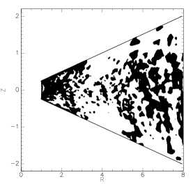
Figure 3: Left panel: Time and azimuthally averaged radial velocity for the model $p=-2$. Positive velocities are marked with white colors, while black regions correspond to negative $v_{R}$. The raw simulation data have been averaged in time between $t=400$ and $t=600$. Right panel: The solid line shows the vertical profile of the radial velocity averaged in time between $t=400$ and $t=600$, in the azimuthal direction and in the radial direction between $R=3$ and $R=6$. The dashed lines show the theoretical prediction of Eq. (14) for $\alpha=10^{-2}$ and $5\times 10^{-3}$, respectively . The dotted line simply marks the zero point as a reference.

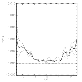
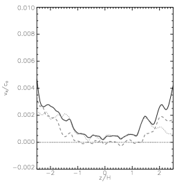
Figure 4: Vertical profile of the radial velocity for the case $p=-2$. In both panels, the solid line is identical to that plotted on the right panel of figure 3 (time average over $[400,600]$ and radial average over $[3,6]$). The left panel investigates the sensitivity of the result on the time average while keeping the same radial range: the time average is taken over $[400,500]$ (dotted line) and $[500,600]$ (dashed line). The right panel shows data obtained with the same time average, $[400,600]$, but different radial range, namely $R\in[2,4.5]$ (dotted line) and $R\in[4.5,7]$ (dashed line).

The properties of the large–scale radial flow that develops during the simulation are illustrated in figure 3. For the results to be easier to interpret, only the region $|Z|<2.5H$ has been considered in the analysis. This corresponds to the midplane region of the disk where most of the mass concentrates. According to Eq. (14), this is also the region where meridional circulation is expected to develop. Velocity fluctuations above that height are so large that no converged mean flow could be extracted from the simulations, even after averaging for $200$ orbits. In any case, because of the exponential drop in density, little mass flux is expected in that region. The sign of the radial velocity in the $(R,Z)$ plane is displayed in the left hand panel of figure 3. Despite the very long averaging period, the patchy structure apparent in that figure indicates that the data remain very noisy even after the long average we performed. As discussed above, this is due to the large–scale flow having an amplitude much smaller than the turbulent velocity fluctuations. Nevertheless, it is also evident from the figure that the numerical simulations do not show any obvious signature of a meridional circulation. Such a feature would have been characterized by a large white region around the disk midplane sandwiched between two black regions. In fact, it appears that many black blobs are clustered around the disk midplane, while the disk surface (i.e. the region located at larger $|Z|$) appears whiter. This is confirmed by the right hand panel of that figure, in which an additional radial averaging has been performed between $R=3$ and $R=6$. The resulting vertical profile of $v_{R}$ is compared with the theoretical expectation of Eq. (14) for two values of $\alpha$, namely $5\times 10^{-3}$ and $10^{-2}$. In the simulations, $v_{R}$ is found to be low in the vicinity of the disk midplane and rises in the disk surface layers. It is surprising to see positive velocities at all $Z$ since it indicates a mean bulk motion of the disk. This will be largely addressed in section 5.2 where the connections between the present simulations and vertically averaged $\alpha$–disks are discussed. Here, we only comment that the large difference between the simulations and the predictions of viscous disk theory further supports the conclusion suggested above. There is no meridional circulation in turbulent protoplanetary disks in which turbulence is driven by the MRI.

As mentioned above, the amplitude of the large–scale flow is nevertheless much smaller than the typical turbulent velocity fluctuations. This raises the question of the uncertainty on the radial velocity vertical profile shown in the right hand panel of figure 3. To investigate this point, we have varied the intervals over which the time and radial averages are performed. The result is shown in figure 4. In both panels, the solid curve is identical to the one plotted in the right hand panel of figure 3: the time average is performed over the range $[400,600]$ and the radial average over the range $[3,6]$. In the left hand panel, the dotted and dashed lines retain the same radial range, $R\in[3,6]$, while the time interval is respectively varied over the range $[400,500]$ and $[500,600]$. In the right hand panel, the time average is performed over the range $[400,600]$ while the radial average is done over $[2,4.5]$ and $[4.5,7]$. As a result, all of these additional curves are obtained by averaging the simulation results either over a smaller radial extent or over a shorter time interval than used to compute the solid curve. They are thus expected to be less converged than the solid line. Nevertheless, the dotted and dashed curves in both panels are qualitatively similar to the solid line (i.e. no meridional circulation is found) and show only moderate quantitative difference with the solid line, indicating that the results shown in figure 3 are converged fairly well.

3.2.3 Turbulent vs. viscous torques

Figure 5: Left panel: Vertical profile of $T_{Z\phi}^{turb}/P_{mid}$ (solid line) and $T_{Z\phi}^{visc}/P_{mid}$ (dashed line), time averaged between $t=400$ and $t=600$ and radially averaged between $R=3$ and $R=6$. The two stresses are similar both in amplitude and in their vertical profile. Right panel: Vertical profile of $T_{R\phi}^{turb}/P_{mid}$ (solid line) and $T_{R\phi}^{visc}/P_{mid}$ (dashed line), time averaged between $t=400$ and $t=600$ and radially averaged between $R=3$ and $R=6$. Although they are comparable in magnitude, the viscous and turbulent stresses display largely different vertical profiles.

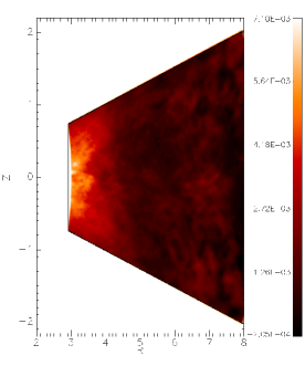
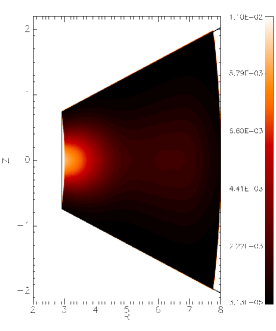
Figure 6: Left panel: Spatial variation of $T_{R\phi}^{turb}/P_{mid}$ in the disk’s meridional plane, time–averaged between $t=400$ and $t=600$. Right panel: Same as the left panel, but for the quantity $T_{R\phi}^{visc}/P_{mid}$. A strong vertical stratification is apparent in the viscous stress but appears to be much weaker in the turbulent stress.

The results presented above demonstrate important differences between the large–scale flow properties of viscous and turbulent disks. This is due to differences between viscous and turbulent stresses. Indeed, as outlined in section 2.4, stress tensors responsible for angular momentum transport have no reason to be identical in viscous and in turbulent disks. We now compare them in detail.

We first consider the $Z\phi$ components of those stresses. Both $T_{Z\phi}^{visc}$ and $T_{Z\phi}^{turb}$ are respectively given by Eq. (12), along with the $\alpha$–prescription for the viscosity and Eq. (17). The left hand panel of figure 5 compares the vertical profile of $T_{Z\phi}^{turb}/P_{mid}$ and $T_{Z\phi}^{visc}/P_{mid}$. As for the right hand panel of figure 3, the simulation data have been averaged in azimuth over the entire computational domain and in radius between $R=3$ and $R=6$. A further average over $11$ snapshots evenly spaced between $t=300$ and $t=600$ was also performed. The two stresses display a comparable amplitude and a similar vertical profile, which is ultimately related to the sign and the amplitude of the vertical derivative of $\Omega$.

We now turn our attention to the $R\phi$ components of the viscous and turbulent stress tensors. These are given by Eq. (11), along with the $\alpha$–prescription for the viscosity, and Eq. (16), respectively. Snapshots of both tensors in the disk’s meridional plane, properly averaged in time and azimuth, are shown in figure 6. The left hand panel shows $T_{R\phi}^{turb}/P_{mid}$ while the right hand panel plots $T_{R\phi}^{visc}/P_{mid}$ (as for the left panel of figure 3, only the region within $2.5$H of the equatorial plane has been plotted here). First, both the viscous and turbulent $R\phi$ components of the stress are much larger in amplitude than the $Z\phi$ components plotted in the left hand panel. Second, their vertical profiless are markedly different. While $T_{R\phi}^{turb}$ vertical variations are weak, those of $T_{R\phi}^{visc}$ are strong. This is because the latter traces the large vertical gradient of the gas density, while the former arises mainly because of magnetic forces. This difference is made even more apparent in the right hand panel of figure 5 in which a further radial average between $R=3$ and $R=6$ has been performed. (The range of the x–axis has been expanded up to $4.5H$ compared to figure 6.) In this figure, the solid line plots the turbulent stress while the dashed line represents the viscous stress tensor. As suggested by figure 6, the viscous stress displays a vertical profile reminiscent of the Gaussian density profile. The turbulent stress, because it is dominated by the magnetic forces, shows a plateau for $|Z|<2.5H$ before dropping to lower values higher in the disk. Such a vertical profile for the turbulent stress tensor has already been reported in numerous numerical simulations of MRI–driven MHD turbulence, using either a local (Miller & Stone 2000; Hirose et al. 2006; Flaig et al. 2010) or a global approach (Fromang & Nelson 2006; Dzyurkevich et al. 2010; Sorathia et al. 2010). As becomes clear in section 5.1, it is precisely this peculiar vertical structure in the turbulent stress that prevents meridional circulation from developing.

3.3 Dependence with the surface density power law index

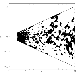
Figure 7: Same as figure 3 but for the case $p=-5/2$.

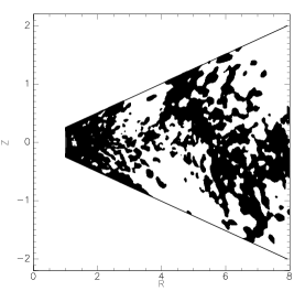
Figure 8: Same as figure 3 but for the case $p=-3/2$.

Even though the previous results suggest a significant difference between viscous and turbulent models, the simulations presented above still display large fluctuations. To assess the robustness of the result, namely the absence of any meridional circulation in turbulent disks, we present in this section two additional simulations for which $p=-3/2$ and $p=-5/2$. These two runs serve two purposes: first, they probe different disk radial structure. Second, and maybe more importantly, they test the nature of the large–scale flow in disks given different realizations of the turbulent flow.

The results of these two simulations are displayed in figures 7 and 8 for the case $p=-5/2$ and $p=-3/2$, respectively. Both figures are similar to figure 3: the left hand panel shows the meridional distribution of $v_{R}$, with white regions corresponding to outward motions and black regions to inward flow; the right hand panel plots the vertical profile of $v_{R}$ radially averaged between $R=3$ and $R=6$. This is compared to the predictions of viscous disk theory (depicted using a dashed line). Both models confirm the differences between turbulent and viscous disks. No meridional circulation is observed, and the results are similar to the fiducial model $p=-2$. The absence of meridional circulation in turbulent protoplanetary disks thus appears quite general (i.e. independent of the disk structure).

4 Numerical checks

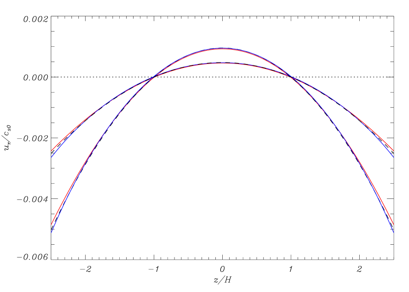
Figure 9: Vertical profile of the gas radial velocity obtained in two hydrodynamical viscous simulations with the Pencil code (red solid line) and with the JUPITER code (solid blue line). The two sets of curves plot the simulations results obtained with $\alpha=5\times 10^{-3}$ and $10^{-2}$ while the dashed lines are the analytical predictions of Eq. (14). Numerical and analytical results are in excellent agreement with each other.

The MHD simulations presented in the section above suggest that meridional circulation is not present in turbulent protoplanetary disks. However, because of its very small amplitude, one has to be careful since a number of potential numerical issues might affect this conclusion. For example, the grid meridional boundaries might cause wave reflections that could perturb the development of that circulation, while the limited radial extent of the computational domain perturbs its viscous evolution. Both problems can potentially affect the development of meridional circulation. To address these issues, we have used two hydrodynamic codes, namely the Pencil Code and the code JUPITER (de Val-Borro et al. 2006). Both codes were used to solve the hydrodynamic equations in spherical geometry with a prescribed kinematic viscosity. The implementation of the viscous force in both codes was checked using the test described in Appendix A. At $t=0$, a disk in hydrostatic equilibrium is initialized as described in section 2.2, using $q=-1$, $p=-2$, and $H_{0}/R_{0}=0.1$. The $\alpha$ prescription is used with the two different values $\alpha=5\times 10^{-3}$ and $10^{-2}$. The size of the grid and the resolution in the disk’s meridional plane are identical to the MHD runs performed with GLOBAL. However, the boundary conditions differ. The Pencil simulation was done with periodic boundaries in $\theta$. JUPITER in turn used simple reflexive boundary conditions both in colatitude and radius, so that the ghost zones are filled with copies of the neighboring zones of the active mesh, using a mirror symmetry. This yields a trivial Riemann problem at the boundary, hence a zero mass flux and a momentum flux that scales with the pressure at the boundary.

The results obtained with the two codes are summarized in figure 9, in which the vertical profile of the radial velocity is plotted for the two values of $\alpha$ quoted above. All curves are averaged in azimuth and in radius between $R=3$ and $R=6$. They were obtained at times $t=250$ (Pencil Code results), $t=37.5$ (Jupiter results, case $\alpha=5\times 10^{-3}$) and $t=57.5$ (Jupiter results, case $\alpha=10^{-2}$). For both codes and both values of $\alpha$, the agreement between the numerical results and the analytical predictions is spectacular. There is only a tiny mismatch above $2H$, which is most likely due to the meridional boundary conditions. This remarkable agreement shows that meridional circulation, when it exists, is a robust feature of the flow that is easily recovered in numerical simulations. It is neither affected by the presence of artificial boundaries nor strongly influenced by the details of the numerical algorithm. In addition, these results are obtained at much shorter times than the disk’s viscous timescale at $R=4.5$. Indeed the later amounts to a few hundreds orbits, while the results are obtained after a few tens of orbital times at that radius. This confirms the claims of Kley & Lin (1992) and Rozyczka et al. (1994) that meridional circulation is established quickly, i.e. on a much shorter timescale than the disk’s viscous timescales. As a conclusion, these viscous disk numerical simulations give further confidence that the lack of meridional circulation reported in section 3 is a real feature of turbulent protoplanetary disks.

5 Discussion

The numerical simulations presented above have shown striking differences between viscous and turbulent disks. In this section, we first present a simple model that accounts for the numerical results and discuss the relationship between these results and 1D standard $\alpha$ disk models before highlighting the consequences of our findings for large–scale radial transport of solids in protoplanetary disks.

5.1 A simple model

Figure 10: The solid line shows the vertical profile of $v_{R}$ for the case $p=-2$, derived as described in figure 3. It should be compared with the dashed line which plots the prediction of Eq. (25), using $\alpha_{t}=5\times 10^{-3}$ and $H_{0}/R_{0}=0.1$.

Figure 11: Same as figure 10, but for the cases $p=-3/2$ (top panel) and $p=-5/2$ (bottom panel).

In section 3.2.3, it was shown that meridional circulation fails to be established in turbulent protoplanetary disks. As explained in section 3.2.3, this behavior, unlike that of viscous disks, is due to differences between the viscous and turbulent stress tensors that are responsible for angular momentum transport. In this section, we provide a simple prescription for the turbulent stresses $T_{R\phi}^{turb}$ and $T_{Z\phi}^{turb}$ that accounts for the 2D structure of the large–scale flow observed in the simulations.

First, the right hand panel of figure 5 shows that the $R\phi$ component of the turbulent and viscous stress tensors are comparable in amplitude. In addition, both stresses are larger by about an order of magnitude than the $Z\phi$ components of the stress $T_{Z\phi}^{visc}$ and $T_{Z\phi}^{turb}$ (compare the vertical scales on the two panels of that figure). This suggests that the $Z\phi$ component of the stress is not a fundamental piece in the process of setting the flow topology. For example, in the derivation of the radial velocity in section 2.3, the $R\phi$ contribution of the viscous stress to the meridional variations of the radial velocity writes as

$$\frac{v_{R}^{(R\phi)}}{c_{0}}=-\alpha\left(\frac{H_{0}}{R_{0}}\right)\left(\frac{R}{R_{0}}\right)^{q+1/2}$$ (20)

$$\hskip 56.9055pt\left[3p+3q+6+\frac{3q+9}{2}\left(\frac{Z}{H}\right)^{2}\right]\,.$$

This last expression is very similar to the complete expression for $v_{R}$ that is given by Eq. (14) and still indicates outward motion in the disk midplane and inward motion in the disk upper layers for a wide range of $p$ and $q$ values. Obviously, the essence of the meridional circulation lies in the $R\phi$ component of the viscous stress. We thus adopt, for simplicity, the following prescription for the $Z\phi$ component of the turbulent stress:

$$T_{Z\phi}^{turb}=0\,.$$ (21)

The conservation of angular momentum, Eq. (15), can thus be written as

$$R\rho v_{R}\frac{\partial R^{2}\Omega_{K}}{\partial R}=\frac{\partial}{\partial R}\left(R^{2}T_{R\phi}^{turb}\right)\,,$$ (22)

where the vertical velocity has been dropped as it is an order $H/R$ lower than the radial velocity. Similarly, the vertical variation in $\Omega$ appearing on the left hand side of the equation above has been neglected because it would result in terms of order $(H/R)^{2}$, i.e. much smaller than the vertical variations arising as a result of the vertical density stratification. Using the variations for the gas density given by Eq. (6), Eq. (22) can then be written as

$$\frac{v_{R}}{c_{0}}=2\left(\frac{H_{0}}{R_{0}}\right)\left(\frac{R}{R_{0}}\right)^{-p-1/2}\frac{\partial}{\partial R}\left(R^{2}T_{R\phi}^{turb}\right)$$ (23)

$$\hskip 113.81102pt\frac{1}{R_{0}\rho_{0}c_{0}^{2}}\exp\left(+\frac{Z^{2}}{2H^{2}}\right)\,.$$

In the bulk on the disk ($|Z|<2.5H$), the results of the simulations (figures 5 and 6) demonstrate that $T_{R\phi}^{turb}$ is largely independent of $Z$. Thus the only dependence with $Z$ in the expression above is in the exponential, which explains why the sign of the radial velocity does not depend on the distance to the midplane.

Whether the radial velocity is positive or negative instead depends on the radial derivative of the turbulent stress tensor. If the radial variations of $T_{R\phi}^{turb}$ are steeper than $R^{-2}$, $v_{R}$ is negative everywhere. In the opposite situation, it is positive, as found in the simulations presented in this paper. For illustrative purposes, we adopt in the following a simple power–law radial dependence for $T_{R\phi}^{turb}$ and writes:

$$T_{R\phi}^{turb}=\left\{\begin{array}[]{ll}-\alpha_{t}\rho_{0}c_{0}^{2}\left(\frac{R}{R_{0}}\right)^{\delta}&\textrm{if }|Z|<2.5H\\ 0&\textrm{otherwise}\end{array}\right.\,.$$ (24)

Such a prescription bears similarities to the one adopted by Kretke & Lin (2010) in their disk models. In Eq. (24), $\alpha_{t}$ is a normalizing factor of the stress that shall not be thought of as the standard $\alpha$ parameter. However, on dimensional grounds, $\alpha_{t}$ and $\alpha$ are expected to have the same order of magnitude. The power–law exponent $\delta$ is an unknown number that depends a priori on the disk properties (for example the density and sound speed exponents $p$ and $q$). It is important, at this stage, to stress that such a form in the radial variations of the stress tensor has absolutely no theoretical grounds and should only be viewed as a means to pushing the analysis further. Using the expression above for the stress tensor, the radial velocity of the gas can be written as

$$\frac{v_{R}}{c_{0}}=-2\alpha_{t}(\delta+2)\left(\frac{H_{0}}{R_{0}}\right)\left(\frac{R}{R_{0}}\right)^{\delta-p+1/2}\exp\left(\frac{Z^{2}}{2H^{2}}\right)$$ (25)

when $|Z|<2.5H$, while $v_{R}$ vanishes in the disk’s upper layers. The results of the simulations presented in this paper show that $v_{R}$ is positive in the disk midplane, suggesting $\delta<-2$ for the set of disk parameters probed in the present paper. It would be tempting at this stage to take the actual measured radial variations in the stress instead of using the simple power law given by the equation above. We chose not to do it for two main reasons: first, as detailed in the following sections, these variations may be polluted by numerical artifacts and thus may not be representative of an actual protoplanetary disk, and second, whether a meridional circulation develops does not depend on those variations, as shown by Eq. (23). Rather, we simply observe that the results of the simulations indicate a midplane radial velocity on the order of $5\times 10^{-4}c_{0}$. In other words, it is around $\alpha(H_{0}/R_{0})$. This suggests in turn that $2(\delta+2)(R/R_{0})^{\delta-p+1/2}$ is close to unity. Eq. (25) for the radial velocity is compared with the simulation results, for the case $p=-2$, in the left hand panel of figure 10. In computing $v_{R}$ using that equation, we have used $\alpha_{t}\sim\alpha\sim 5\times 10^{-3}$, $H_{0}/R_{0}=0.1$ while the remaining terms (with the exception of the exponential!) are assumed to be equal to one. Given the simplicity of the prescriptions detailed above, the agreement between the simulation results and the prediction of Eq. (25) is very good.

Finally, the prediction of Eq. (25) is further compared with the simulation results for the case $p=-3/2$ (top panel) and $p=-5/2$ (bottom panel) in figure 11. Again, the agreement between the simulations and the prediction of Eq.(25) is satisfactory for the case $p=-5/2$, while the case $p=-3/2$ shows larger, but still modest deviations from the simple analytical prediction.

5.2 Comparison with the predictions of standard $\alpha$ disk models

Standard 1D $\alpha$ disk theory considers the height and azimuthally integrated version of Eq. (10) to describe angular momentum transport. (All $Z$–derivatives disappear in that procedure.) Using the notation introduced in section 3.2.1, it is expressed as (Papaloizou & Lin 1995; Balbus & Papaloizou 1999)

$$R\Sigma\overline{v_{R}}\frac{d}{dR}\left(R^{2}\Omega\right)=\frac{d}{dR}\left(R^{2}\Sigma\overline{T_{R\phi}^{visc}/\rho}\right)\,.$$ (26)

Assuming it has the form of a standard viscous stress tensor, the height and azimuthally integrated $R\phi$ component of the stress are then

$$\Sigma\overline{T_{R\phi}^{visc}/\rho}=\frac{1}{2\pi}\int T_{R\phi}^{visc}d\phi dz=\frac{1}{2\pi}\overline{\nu}\Sigma R\frac{d\Omega}{dR}\,.$$ (27)

Standard $\alpha$ disk models then make the ansatz that it is in fact the vertically and azimuthally average kinematic viscosity $\overline{\nu}$ that takes the form given by Eq. (9). This is different from the theory developed in section 2.3, where this relation is assumed to hold locally. Using that prescription for $\overline{\nu}$ in Eq. (27) and given the radial dependence of the Keplerian angular velocity, the vertically and azimuthally averaged stress tensor writes as

$$\Sigma\overline{T_{R\phi}^{visc}/\rho}=\frac{1}{2\pi}\int T_{R\phi}^{visc}d\phi dz=-\frac{3}{2}\alpha\Sigma c_{s}^{2}\,.$$ (28)

For locally isothermal disks such as those considered in the present paper, this relation can be equivalently expressed in terms of the thermal pressure as

$$\int T_{R\phi}^{visc}d\phi dz=-\frac{3}{2}\alpha\int Pd\phi dz\,.$$ (29)

This equation shows that the relation between stress and pressure holds for vertically integrated quantities in standard $\alpha$ disk theory, while the model developed in section 2 explicitly assumes that it holds locally: $T_{R\phi}^{visc}=-3/2\alpha P$. The results presented in this paper have shown that such a local relation does not hold between the turbulent stress and the thermal pressure, as it would otherwise result in meridional circulation developing in turbulent disks. Nevertheless, this does not mean that this relation would not hold between the vertically averaged turbulent stress and the vertically averaged thermal pressure, as is the case in standard $\alpha$ disk theory as shown by Eq. (29).

A first attempt at answering this question can be made by comparing the vertically and azimuthally averaged radial velocity predicted, on one side, by 1D $\alpha$ disk model and, on the other hand, by the numerical simulations of protoplanetary disks presented in this paper. In standard 1D $\alpha$ disk models, the radial profile of the vertically integrated radial velocity can be computed by plugging Eq. (29) into Eq. (26) to get

$$\frac{\overline{v_{R}}}{c_{0}}=-3\alpha\left(\frac{H_{0}}{R_{0}}\right)\left(\frac{R}{R_{0}}\right)^{q+1/2}\left[p+\frac{3q}{2}+\frac{7}{2}\right]\,.$$ (30)

Equation (30) can also be recovered from Eq. (14) by a simple vertical integration (Takeuchi & Lin 2002). For the value $q=-1$ considered in the present paper, it vanishes and changes sign for $p=-2$. When $p<-2$, Eq. (30) predicts a positive vertically integrated radial velocity, while $\overline{v_{R}}$ is negative for $p>-2$. This behavior is different from what is found in the simulations, in which outward bulk motions were observed regardless of the value of $p$. This suggests that turbulent disk behave differently than standard 1D $\alpha$ disk models.

The systematic outward velocities obtained in the simulations can be traced back to $\alpha$ not being a constant function of R, but rather systematically decreasing outward. Indeed, when using the prescription for the turbulent stress tensor given by Eq. (24), $\alpha=\overline{T_{R\phi}^{turb}/\rho}/\overline{c_{s}^{2}}$ as given by Eq.(18), is found to scale like $R^{\delta+2}$. Constant $\alpha$ values thus correspond to disk regions where $\delta=-2$. In constrast, $\delta<-2$ in those parts of the disks where $\alpha$ decreases with R. Using Eq. (25), we can thus predict outward midplane radial velocities in the region where $\alpha$ decreases radially (since $\delta+2<0$ there). The tendenct of $\alpha$ to decrease with $R$ in our simulations thus explains the trend toward finding positive midplane radial velocities. As shown by figure 1, in model $p=-2$, $\alpha$ is almost constant in the region $R\in[4.5,7]$. In this region, we thus expect to have $\delta\sim 2$, and Eq. (25) predicts a vanishing radial velocity in the disk midplane. This is again consistent with the simulation results, as shown in the right hand panel of figure 4. Finally, Eq. (25) predicts that negative midplane radial velocities are obtained when $\delta>-2$, or equivalently when $\alpha$ increases outward. We note that this prediction is consistent with the recent results of Flock et al. (2011). In simulations similar to those presented here, these authors indeed reports radially increasing $\alpha$ and inward radial velocities.

The systematic positive radial velocities we report here might appear suspicious for the long term evolution of an accretion disk, so it deserves a comment. We start by stressing that $\alpha$ disk models such as those used here also exhibit that property for some combination of the exponents $p$ and $q$. This is the case for example of the model $q=-1$ and $p=-2.5$, for which Eq. (30) predicts a positive velocity implying outward mass transport. This can only be a transient situation. The mass accretion rate $\dot{M}=-2\pi R\Sigma v_{R}$ is negative in this case and scales like $R^{p+3q/2+3}$. Thus its exponent is negative, showing that the mass accretion rate and its derivative both decrease with $R$ in amplitude. On viscous timescales, the radial profile of $\Sigma$ will flatten and accretion will proceed. Ultimately, mass will fall onto the star as angular momentum is transported outward. Although it is currently impossible to run 3D MHD simulations on viscous disk timescales, the same is most likely true of the turbulent disk that is simulated in the present paper. We would thus expect to recover accretion if the simulations were run long enough. However, this does not prevent a comparison between viscous models and simulations when disks are not in steady state, because the mean flow in disks is established on a shorter timescale than the viscous timescale. The point of the present section is precisely to highlight that the predictions of standard $\alpha$ disk theory differ from the findings of numerical simulations. That being said, we caution that these simulations only probe such differences for the limited time and parameters enabled by current computational resources. Whether they are general is beyond the scope of this paper and should be the focus of future work.

We finally comment that the differences we report between turbulent and standard $\alpha$ disk model are consistent with previous results in the literature. For example, Sano et al. (2004) report a scaling of the turbulent stress tensor as $P^{1/4}$, and not as $P$ as in standard $\alpha$ disk theory. This is consistent with the simulations of Lyra et al. (2008). Along the same lines, Hirose et al. (2009) have also recently reported the lack of a direct relation between stress and thermal pressure using shearing box simulations of turbulent disks. At the same time, the results presented in the present paper regarding this question should be taken with care. Recent studies have shown that the saturation level of the MRI in the unstratified shearing box is strongly affected by explicit dissipation (Lesur & Longaretti 2007; Fromang et al. 2007; Simon & Hawley 2009). In the simulations presented here, all the dissipation is of numerical origin. Thus numerical dissipation alone could mask any scaling of the stress with the disk parameters. To make things even worse, numerical dissipation in these simulations is in principle a function of position since the effective radial resolution per disk scaleheight varies with radius. Any definite conclusions regarding the precise scaling of the vertically averaged stress with pressure should thus wait for better control of dissipation in global simulations, a difficult task by definition. The present results highlight once more the need for an accurate determination of the saturation of the turbulent stress as a function of the disk parameters. Such a task is beyond the scope of the present paper but should also be the focus of future work.

5.3 Conclusions

Large–scale meridional circulation has been predicted in protoplanetary disks based on 2D viscous disk theory. However, the flow in a protoplanetary disk is known to be turbulent, most likely because of the MRI. The question raised in this paper is thus simple: does meridional circulation exist in turbulent protoplanetary disks? This problem has been addressed using a set of numerical simulations of turbulent protoplanetary disks. The large–scale radial flow of the gas was computed by averaging the results in the azimuthal direction, as well as on long time intervals. The results are found to disagree with 2D viscous disk theory. There is no sign of any meridional circulation in the disk. Instead, the sign of the radial velocity is found to be constant in the bulk of the disk ($|Z|<2.5H$). This is shown to come from the vertical behavior of the turbulent stress tensor. Instead of scaling like the local thermal pressure as assumed in 2D viscous disk theory, the turbulent stress is constant around the disk midplane before dropping in the disk corona, where thermal and magnetic pressure become comparable. Such a vertical profile of the turbulent stress has been found already in many numerical simulations, regarless of their local and global nature. It is thus a robust property of the flow in turbulent disks. In light of these properties of the stress, the conclusion that no meridional circulation exists in fully ionized and turbulent protoplanetary disks appears unavoidable.

This has important consequences for the transport of solids in the solar nebula. The relevance of models in which crystalline dust radial transport is largely based on meridional circulation can be questioned (Keller & Gail 2004; Tscharnuter & Gail 2007; Ciesla 2007, 2009; Hughes & Armitage 2010). In addition, the simulations also raise the possibility of an outward radial mass flux unexpected from a standard $\alpha$ disk model. This opens up the possibility of an efficient mechanism to transport solid particles outward. Given the current state of the art of global numerical simulations of protoplanetary disks, the viability of such a feature of the flow nonetheless remains very uncertain. Future studies of MRI–powered MHD turbulence should aim at better constraining the nature of the large–scale flow in disks and the saturation amplitude of the MRI as a function of the disk’s properties (surface densities, temperature).

It is also important to realize that the simulations presented here do not rule out the possibility of a large–scale outward flow in protoplanetary disks. They only demonstrate it does not exist in fully turbulent disks and that a viscous modeling of such disks leads to erroneous results. There are a number of possibilities by which a meridional flow might develop in real protoplanetary disks. First, protoplanetary disks are known to be largely neutral and most likely harbor a dead zone around their equatorial plane in which the flow is stable to the MRI. While the exact size and dynamical status of the dead zone is uncertain because it depends both on chemical (Fromang et al. 2002; Ilgner & Nelson 2006b, a) and dynamical effects (Fleming & Stone 2003; Turner et al. 2007; Ilgner & Nelson 2008), its very existence in the planet–forming region seems difficult to avoid. The large–scale flow in such disks has never been considered and might lead to unexpected results that could affect the large–scale transport of solid particles. For example, Bai & Stone (2010) recently showed that the fast inward drift of large particles causes an outflow of gas in the dead zone midplane that could carry small solids like CAIs with it. Finally, one should bear in mind the idealized nature and the limited sampling of the parameter space of the simulations presented here. Additional physical ingredients (ambipolar diffusion, hall effects) or different disk properties (temperature radial and vertical profile, magnetic field configuration) might all change the vertical profile of the stress tensor and create a large scale outflow in the bulk of the disk.

Appendix A Off-centered Keplerian viscous ring spreading in spherical geometry

o To test the implementation of the viscous stress tensor in our purely hydrodynamical codes, we have designed a set up, in spherical coordinates $(r,\theta,\phi)$, in which the two components of the stress tensor that potentially contribute to meridional circulation are within the same order of magnitude. It consists of a disk orbiting within a fixed potential $\Phi$ that has the following form:

$$\Phi(r,\theta,\phi)=-\frac{GM}{r\sin\theta}+\lambda(r\cos\theta-Z_{0})^{2},$$ (31)

where $Z_{0}$ and $\lambda$ are constants. This potential is Keplerian along the cylindrical radius $R=r\sin\theta$, and harmonic in the vertical direction $Z=r\cos\theta$, with a potential minimum at $Z_{0}\neq 0$. An equilibrium setup for this potential can therefore correspond, for a globally isothermal gas with sound speed $c_{s}$, to an approximately Keplerian disk with its equator lying at $Z=Z_{0}$ and with a uniform thickness given by $H=c_{s}/\omega_{z}$, where $\omega_{z}^{2}=\partial^{2}\Phi/\partial z^{2}=2\lambda$. Namely, we initialize our disk as

$$\rho(r,\theta,\phi) = \frac{m}{2\pi^{2}R_{0}^{2}H\sqrt{2\tau_{0}}}x^{-3/4}\times$$

$$\exp\left[-\frac{(x-1)^{2}}{\tau_{0}}-\frac{(Z-Z_{0})^{2}}{2H^{2}}\right],$$

where $x=R/R_{0}$ and $\tau_{0}=12\nu t/R_{0}^{2}$, which is the ratio of the time and of the viscous timescale of the disk (Lynden-Bell & Pringle 1974). $\tau_{0}$ is set to be much lower than unity in the expression above. Equation (A) corresponds to a narrow Gaussian ring of mass $m$, centered on $R_{0}$, in vertical hydrostatic equilibrium, so that it also has a Gaussian profile, centered on $Z_{0}$, in the vertical direction. Eq. (A) stems from the classical expression of Lynden-Bell & Pringle (1974), which describes the radial spread of an initially infinitely narrow viscous ring, in which we approximate the Bessel function $I_{1/4}(2x/\tau_{0})$ with $\exp(2x/\tau_{0})/\sqrt{4\pi x/\tau_{0}}$, using the fact that its argument $2x/\tau_{0}$ is large. This means that we start with a ring that has already undergone some viscous radial spread, although for a time short compared to its viscous timescale, so that its width is small compared to its radius. A meridional cut of the initial density field is represented in Figure 12.

We initialize the azimuthal velocity as follows:

$$v_{\phi}=\left\{\frac{GM_{*}}{R}-c_{s}^{2}\left[\frac{3}{4}+\frac{2(x-1)x}{\tau_{0}}\right]\right\}^{1/2},$$ (33)

where the last two terms correspond to the rotational support provided by the radial pressure gradient, and we initialize the cylindrical radial velocity as

$$v_{R}=\frac{\nu}{R}\left[\frac{3}{4}+\frac{6}{\tau_{0}}x(x-1)\right],$$ (34)

from which we set $v_{r}=v_{R}\sin\theta$ and $v_{\theta}=v_{R}\cos\theta$. Equation (34) stems from Eq. (13), in which the $Z$ derivative is set to $0$, as no vertical dependence of $\Omega$ is expected in this setup, each layer at a given altitude being a replica of the equatorial layer, with a density ratio that depends on the altitude.

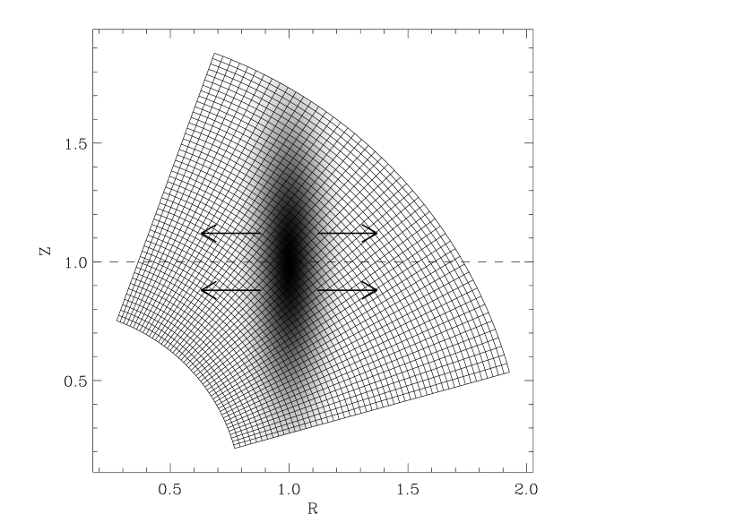
Figure 12: Initial density field (gray levels) superimposed on the spherical mesh used in the calculation. The dashed line represents the “equator” (i.e. the potential minimum in the $Z$ direction), while the thick arrows depict the expected trend of the ring’s material to spread radially.

For our fiducial calculation, we adopt $c_{s}=10^{-3/2}(GM/R_{0})^{1/2}$, $\lambda=10^{-2}/3(GM/R_{0}^{3})$, hence $H=\sqrt{0.15}R_{0}$, and we start with a narrow ring corresponding to $\tau_{0}=0.018$, with an equator at $Z_{0}=1$. Our mesh contains $50\times 50$ zones, regularly spaced in radius from $R=0.8R_{0}$ to $R=2R_{0}$, and regularly spaced in colatitude from $\theta=0.35$ to $\theta=1.3$. Since the azimuthal velocities are taken into account, our setup is “2D1/2” in nature.

Figure 13: Equatorial density cuts for $\tau_{0}=0.018$ (initial conditions, highest and narrowest peak), $\tau_{0}=0.04$ and $\tau_{0}=0.09$ (widest distribution). In each case the diamond’s curve represents the distribution inferred in the $Z=Z_{0}$ plane from the numerical simulations, using a bilinear interpolation, while the solid curve represents the exact solution of Lynden-Bell & Pringle (1974). In addition, the dotted and dashed curves represent the situation obtained for $\tau_{0}=0.09$ in numerical calculations in which we set $T^{\rm visc}_{\theta\phi}$ and $T^{\rm visc}_{r\phi}$ to zero, respectively.

We present in Figure 13 the results of this calculation, which show that the radial spread of the ring is correctly captured on the spherical mesh. We performed subsidiary calculations in which we manually cancel out one of the two stress components that have an impact on the torque felt by a ring of material (hence on the rate at which the material spreads), i.e. either $T^{\rm visc}_{\theta\phi}$ or $T^{\rm visc}_{r\phi}$. That the resulting curves of these two additional calculations display a significantly different result than the correct result and that they yield a similar peak value at the same date shows that these two components of the stress tensor play roles of comparable magnitude on the spread of the ring. This can be understood as the spherical coordinate system, in the vicinity of the center of the ring at $Z=Z_{0}$, is approximately tilted by $45^{\circ}$ with respect to the equator. We finally note that the original derivation of Lynden-Bell & Pringle (1974) does not contemplate pressure effects. Those are relatively substantial in the disk considered here, and might account for the tiny discrepancy between the simulated and expected profiles in Figure 13, except near the boundaries, where the discrepancy likely arises from the accumulation of material due to the reflexive boundary conditions that we use, which prevent material from flowing out of the grid.

References

- Bai & Stone (2010) Bai, X.-N. & Stone, J. M. 2010, ApJ, 722, 1437
- Balbus & Hawley (1991) Balbus, S. & Hawley, J. 1991, ApJ, 376, 214
- Balbus & Hawley (1998) Balbus, S. & Hawley, J. 1998, Rev.Mod.Phys., 70, 1
- Balbus & Papaloizou (1999) Balbus, S. & Papaloizou, J. 1999, ApJ, 521, 650
- Bockelée-Morvan et al. (2002) Bockelée-Morvan, D., Gautier, D., Hersant, F., Huré, J., & Robert, F. 2002, A&A, 384, 1107
- Bouwman et al. (2008) Bouwman, J., Henning, T., Hillenbrand, L. A., et al. 2008, ApJ, 683, 479
- Brownlee et al. (2006) Brownlee, D., Tsou, P., Aléon, J., et al. 2006, Science, 314, 1711
- Ciesla (2007) Ciesla, F. J. 2007, Science, 318, 613
- Ciesla (2009) Ciesla, F. J. 2009, Icarus, 200, 655
- Crovisier et al. (1997) Crovisier, J., Leech, K., Bockelee-Morvan, D., et al. 1997, Science, 275, 1904
- de Val-Borro et al. (2006) de Val-Borro, M., Edgar, R. G., Artymowicz, P., et al. 2006, MNRAS, 370, 529
- Dzyurkevich et al. (2010) Dzyurkevich, N., Flock, M., Turner, N. J., Klahr, H., & Henning, T. 2010, A&A, 515, A70+
- Flaig et al. (2010) Flaig, M., Kley, W., & Kissmann, R. 2010, ArXiv e-prints
- Fleming & Stone (2003) Fleming, T. & Stone, J. M. 2003, ApJ, 585, 908
- Flock et al. (2011) Flock, M., Dzyurkevich, N., Klahr, H., Turner, N. J., & Henning, T. 2011, ArXiv e-prints
- Fromang & Nelson (2005) Fromang, S. & Nelson, R. 2005, MNRAS, 364, L81
- Fromang & Nelson (2006) Fromang, S. & Nelson, R. P. 2006, A&A, 457, 343
- Fromang & Nelson (2009) Fromang, S. & Nelson, R. P. 2009, A&A, 496, 597
- Fromang et al. (2007) Fromang, S., Papaloizou, J., Lesur, G., & Heinemann, T. 2007, A&A, 476, 1123
- Fromang et al. (2002) Fromang, S., Terquem, C., & Balbus, S. A. 2002, MNRAS, 329, 18
- Gail (2001) Gail, H. 2001, A&A, 378, 192
- Hawley & Stone (1995) Hawley, J. & Stone, J. 1995, Comput. Phys. Commun., 89, 127
- Hirose et al. (2009) Hirose, S., Krolik, J. H., & Blaes, O. 2009, ApJ, 691, 16
- Hirose et al. (2006) Hirose, S., Krolik, J. H., & Stone, J. M. 2006, ApJ, 640, 901
- Hu (2010) Hu, R. 2010, ApJ, 725, 1421
- Hughes & Armitage (2010) Hughes, A. L. H. & Armitage, P. J. 2010, ApJ, 719, 1633
- Ilgner & Nelson (2006a) Ilgner, M. & Nelson, R. P. 2006a, A&A, 445, 205
- Ilgner & Nelson (2006b) Ilgner, M. & Nelson, R. P. 2006b, A&A, 445, 223
- Ilgner & Nelson (2008) Ilgner, M. & Nelson, R. P. 2008, A&A, 483, 815
- Keller & Gail (2004) Keller, C. & Gail, H. 2004, A&A, 415, 1177
- Kley & Lin (1992) Kley, W. & Lin, D. N. C. 1992, ApJ, 397, 600
- Kretke & Lin (2010) Kretke, K. A. & Lin, D. N. C. 2010, ApJ, 721, 1585
- Lesur & Longaretti (2007) Lesur, G. & Longaretti, P.-Y. 2007, MNRAS, 378, 1471
- Lynden-Bell & Pringle (1974) Lynden-Bell, D. & Pringle, J. E. 1974, MNRAS, 168, 603
- Lyra et al. (2008) Lyra, W., Johansen, A., Klahr, H., & Piskunov, N. 2008, A&A, 479, 883
- Lyra et al. (2009) Lyra, W., Johansen, A., Zsom, A., Klahr, H., & Piskunov, N. 2009, A&A, 497, 869
- Miller & Stone (2000) Miller, K. A. & Stone, J. M. 2000, ApJ, 534, 398
- Nelson & Papaloizou (2003) Nelson, R. & Papaloizou, J. 2003, MNRAS, 339, 993
- Nelson (2005) Nelson, R. P. 2005, A&A, 443, 1067
- Nelson & Gressel (2010) Nelson, R. P. & Gressel, O. 2010, ArXiv e-prints
- Nelson & Papaloizou (2004) Nelson, R. P. & Papaloizou, J. C. B. 2004, MNRAS, 350, 849
- Olofsson et al. (2009) Olofsson, J., Augereau, J., van Dishoeck, E. F., et al. 2009, A&A, 507, 327
- Papaloizou & Lin (1995) Papaloizou, J. C. B. & Lin, D. N. C. 1995, ARA&A, 33, 505
- Papaloizou & Nelson (2003) Papaloizou, J. C. B. & Nelson, R. P. 2003, MNRAS, 339, 983
- Papaloizou et al. (2004) Papaloizou, J. C. B., Nelson, R. P., & Snellgrove, M. D. 2004, MNRAS, 350, 829
- Regev & Gitelman (2002) Regev, O. & Gitelman, L. 2002, A&A, 396, 623
- Rozyczka et al. (1994) Rozyczka, M., Bodenheimer, P., & Bell, K. R. 1994, ApJ, 423, 736
- Sano et al. (2004) Sano, T., Inutsuka, S., Turner, N. J., & Stone, J. M. 2004, ApJ, 605, 321
- Sargent et al. (2009) Sargent, B. A., Forrest, W. J., Tayrien, C., et al. 2009, ApJS, 182, 477
- Shakura & Sunyaev (1973) Shakura, N. I. & Sunyaev, R. A. 1973, A&A, 24, 337
- Shu et al. (2001) Shu, F. H., Shang, H., Gounelle, M., Glassgold, A. E., & Lee, T. 2001, ApJ, 548, 1029
- Shu et al. (1996) Shu, F. H., Shang, H., & Lee, T. 1996, Science, 271, 1545
- Siemiginowska (1988) Siemiginowska, A. 1988, Acta Astron., 38, 21
- Simon & Hawley (2009) Simon, J. B. & Hawley, J. F. 2009, ApJ, 707, 833
- Sorathia et al. (2010) Sorathia, K. A., Reynolds, C. S., & Armitage, P. J. 2010, ApJ, 712, 1241
- Takeuchi & Lin (2002) Takeuchi, T. & Lin, D. N. C. 2002, ApJ, 581, 1344
- Tscharnuter & Gail (2007) Tscharnuter, W. M. & Gail, H. 2007, A&A, 463, 369
- Turner et al. (2007) Turner, N. J., Sano, T., & Dziourkevitch, N. 2007, ApJ, 659, 729
- Urpin (1984) Urpin, V. A. 1984, Sov. Ast., 28, 50
- Winters et al. (2003) Winters, W. F., Balbus, S. A., & Hawley, J. F. 2003, ApJ, 589, 543
- Wooden et al. (2007) Wooden, D., Desch, S., Harker, D., Gail, H., & Keller, L. 2007, Protostars and Planets V, 815
- Wooden et al. (1999) Wooden, D. H., Harker, D. E., Woodward, C. E., et al. 1999, ApJ, 517, 1034
- Zolensky et al. (2006) Zolensky, M. E., Zega, T. J., Yano, H., et al. 2006, Science, 314, 1735