Approximations for modelling CO chemistry in GMCs: a comparison of approaches

Abstract

We examine several different simplified approaches for modelling the chemistry of CO in three-dimensional numerical simulations of turbulent molecular clouds. We compare the different models both by looking at the behaviour of integrated quantities such as the mean CO fraction or the cloud-averaged CO-to-H₂ conversion factor, and also by studying the detailed distribution of CO as a function of gas density and visual extinction. In addition, we examine the extent to which the density and temperature distributions depend on our choice of chemical model.

We find that all of the models predict the same density PDF and also agree very well on the form of the temperature PDF for temperatures $T>30\;{\rm K}$, although at lower temperatures, some difference become apparent. All of the models also predict the same CO-to-H₂ conversion factor, to within a factor of a few. However, when we look more closely at the details of the CO distribution, we find larger differences. The more complex models tend to produce less CO and more atomic carbon than the simpler models, suggesting that the C/CO ratio may be a useful observational tool for determining which model best fits the observational data. Nevertheless, the fact that these chemical differences do not appear to have a strong effect on the density or temperature distributions of the gas suggests that the dynamical behaviour of the molecular clouds on large scales is not particularly sensitive to how accurately the small-scale chemistry is modelled.

1 Introduction

Carbon monoxide (CO) is a key constituent of the gas making up the giant molecular clouds (GMCs) that are the site of almost all Galactic star formation. Although almost all of the molecular gas mass within a GMC is in the form of molecular hydrogen (H₂), this material is extremely difficult to observe directly, as the temperatures within a GMC are too low to excite even the lowest accessible rotational transition of the H₂ molecule, the quadrupole transition between the $J=2$ and $J=0$ rotational levels. On the other hand, CO does become rotationally excited at GMC temperatures, owing to the much smaller energy separation between its rotational levels. It is readily observed in the millimeter, and is arguably the single most important observational tracer of the state of the gas within the clouds. It also plays an important role as the main molecular coolant of the gas over a wide range in densities (see e.g. Neufeld, Lepp & Melnick, 1995). It is therefore important to understand the distribution of CO within GMCs, and how this relates to the underlying gas distribution.

Unfortunately, this is not a simple task. It has been understood for a long time that the gas within GMCs is typically not in chemical equilibrium (see e.g. Leung, Herbst & Huebner, 1984). More recently, numerical modelling has highlighted the fact that the CO abundance within a given parcel of gas within a GMC is a complex function of the density and temperature of the gas, the local radiation field (modulated by absorption by gas elsewhere in the cloud), and possibly also the dynamical history of the gas (Glover et al., 2010). It has also become increasingly clear that molecular clouds are dynamically complex objects, dominated by supersonic, turbulent motions (see e.g. Mac Low & Klessen, 2004, for a comprehensive overview), and that we ignore the effects of this dynamical complexity at our peril. Therefore, if we want to be able to accurately model the formation and destruction of CO within a GMC, the use of detailed models that treat both the chemistry and the turbulent dynamics in an appropriately coupled fashion seems unavoidable.

However, this presents us with a serious numerical challenge. Even if we focus only on the chemistry of hydrogen, helium, carbon and oxygen, and ignore other elements such as nitrogen or sulphur, there are still a very large number of possible reactions and reactants that we could include in our chemical model. For example, in the 2006 release of the UMIST Database for Astrochemistry (Woodall et al., 2007), there are 2115 such reactions, involving a total of 172 different chemical species. In particular, it is the large number of chemical species that must potentially be handled that is the main source of our problems. If we model the chemical evolution of the gas by using a set of ordinary differential equations (ODEs) to represent the rates of change of the chemical abundances, then we find that the required set of ODEs is generally extremely stiff, containing processes with a wide range of different intrinsic timescales. To evolve this set of ODEs in a numerically stable fashion, we must therefore either evolve them explicitly in time using extremely small timesteps, which is impractical, or evolve them implicitly in time. However, if we adopt an implicit approach, then we find in general that the computational cost of solving the implicit ODEs scales as the cube of the number of species involved, $N_{\rm spec}^{3}$. Therefore, when $N_{\rm spec}$ is large, the cost of solving the chemical rate equations can easily come to dominate the total computational cost, putting strict limits on the size of the problems that can be tackled. In practice, values of $N_{\rm spec}$ as large as 14 can be handled in three-dimensional turbulence simulations at the present day (see e.g. Glover et al. 2010; note that while their model includes 32 distinct chemical species, all but 14 of these are assumed to be in chemical equilibrium, or are trivially derivable from conservation laws), but even in this case, solving the chemical rate equations can take up as much as 90% of the total runtime of the simulation. Scaling up from here to the $N_{\rm spec}=172$ subset of the UMIST database mentioned above remains computationally impractical in three-dimensional simulations.

For this reason, a number of authors have sought to reduce $N_{\rm spec}$ to a more tractable value by identifying and retaining only the most important of the reactions involved in the formation and destruction of CO, as well as making other simplifications that are discussed in later sections. When identifying the key reactions, there is an obvious trade-off between complexity (and hence computational cost) and completeness: the larger the number of possible chemical pathways that we include, the slower the code will run. There are models available in the literature that span a range of different complexities, but until now there has been no comparison of the results produced by these different approaches.

In this paper, we present results from a detailed comparison of several different approximate methods for modelling CO formation and destruction in turbulent molecular clouds that span a range of different complexities. We are interested in particular in establishing which results from simulations of turbulent clouds are highly sensitive to the choice of simplified chemical model, and which are relatively insensitive.

2 Simulation setup

The basic setup of the simulations used here is similar to that described in Glover et al. (2010) and Glover & Mac Low (2011). We use the ZEUS-MP code to model driven magnetohydrodynamical turbulence in a cubical volume, with side length $L=20\>{\rm pc}$, using periodic boundary conditions for the gas. The turbulence is driven using the algorithm described in Mac Low et al. (1998), and the amplitude of the driving is chosen in order to maintain the rms turbulent velocity at $v_{\rm rms}=5\>{\rm km}\>{\rm s^{-1}}$. The initial magnetic field strength is $B_{0}=5.85\>\mu{\rm G}$, and the field is assumed to be initially uniform and oriented parallel to the $z$-axis of the simulation. The effects of self-gravity are not included. The simulations are run for $t=1.8\times 10^{14}\>{\rm s}\simeq 5.7\>{\rm Myr}$, or approximately three turbulent eddy turnover times. We showed in Glover et al. (2010) that this is long enough to allow the CO distribution to settle into a statistical steady state.

We perform two sets of simulations (hereafter denoted as set 1 and set 2) with different initial densities: $n_{0}=100\>{\rm cm^{-3}}$ for set 1 and $n_{\rm 0}=300\>{\rm cm^{-3}}$ for set 2, where $n_{0}$ is the initial number density of hydrogen nuclei. The corresponding mean extinctions are therefore $\bar{A}_{\rm V}=3.3$ and $\bar{A}_{\rm V}=9.9$, respectively, where we have assumed a conversion factor from hydrogen column density to dust visual extinction of $5.348\times 10^{-22}\mbox{ mag cm}^{2}$, appropriate to dust in the cold interstellar medium (ISM). We therefore expect that in both cases, detectable amounts of CO will be produced in the clouds, even though the mean mass-weighted CO abundance should differ by more than an order of magnitude between the two sets of runs (Glover & Mac Low, 2011).

In both sets of simulations, we adopt elemental abundances (by number, relative to hydrogen) of $x_{\rm He}=0.1$, $x_{\rm C}=1.41\times 10^{-4}$ and $x_{\rm O}=3.16\times 10^{-4}$ for helium, carbon and oxygen, respectively. We assume that the hydrogen, helium and oxygen are initially atomic, and that the carbon is initially in singly ionized form throughout the simulation volume.

We set the initial gas temperature to 60 K and the initial dust temperature to 10 K in both sets of simulations. To model the subsequent heating and cooling of the gas and the dust, we use a modified version of the Glover et al. (2010) thermal model, as described in that paper and in the Appendix. Set 1 and set 2 consist of six simulations each, one for each of the chemical models described in Section 3. In the models that include the effects of cosmic rays, we adopt a rate $\zeta_{\rm H}=10^{-17}\>{\rm s^{-1}}$ for the cosmic ray ionization of atomic hydrogen. Finally, to model the effects of the external ultraviolet radiation field, we assume that its strength and shape are the same as those of the standard Draine (1978) field. We illuminate each side of the simulation box using the unattenuated field, and model attenuation within the box due to dust absorption, H₂ self-shielding, CO self-shielding and the shielding of CO by H₂ using the ‘six-ray’ approximation introduced by Nelson & Langer (1997). Full details of this procedure can be found in Glover et al. (2010).

3 Chemical models

3.1 Glover et al. (2010) [G10g, G10ng]

The first model we consider is a slightly modified version of the Glover et al. (2010) chemical model. This consists of 218 reactions amongst 32 species, and so although it is the most complicated of the approximate models included in this study, it nevertheless still represents a considerable simplification compared to a model including the full set of reactions from e.g. the UMIST Database for Astrochemistry. However, Glover et al. (2010) demonstrated that this simplified model could accurately reproduce the results obtained with a far more comprehensive model for several 1D test problems, while at the same time being small enough to be usable in a three-dimensional simulation.

We have made one significant change to the Glover et al. (2010) chemical network: the inclusion of an optional treatment of the effects of the recombination of H⁺, He⁺, C⁺, and O⁺ ions on the surfaces of charged dust grains. We treat these processes using the formalism of Weingartner & Draine (2001), which includes the effects of very small dust grains and polycyclic aromatic hydrocarbons. These grain surface processes are not included in any of the other models that we examine, and in order to understand what effect they have on the outcome of the simulations, we have performed runs both with and without them. In the remainder of the paper, we denote these simulations as G10g and G10ng, respectively.

We have also made a number of modifications to our treatment of the thermodynamic behaviour of the gas, in order to improve our ability to model very cold gas. These improvements are used for all of the models examined here and full details of them are given in the Appendix.

3.2 Nelson & Langer (1997) [NL97]

A much simpler approximation is given by the model proposed by Nelson & Langer (1997), which they used to study the dynamics of low-mass ($M=100$–$400\>{\rm M_{\odot}}$) molecular clouds. In their study, Nelson & Langer (1997) assume that all of the hydrogen is already in the form of H₂, and focus their attention on the conversion of singly ionized carbon, C⁺, to carbon monoxide, CO. Their approximation involves the assumption of direct conversion from C⁺ to CO, and vice versa, which allows them to ignore any intermediate species (such as neutral atomic carbon, C). They assume that the conversion of C⁺ to CO is initiated by the formation of an intermediate hydrocarbon radical (e.g. CH or CH₂), which they denote as CH_x. This may then react with oxygen to form CO, or be photodissociated by the interstellar radiation field. Once CO has formed, it is then only destroyed by photodissociation, yielding C and O, but the neutral carbon produced in this way is assumed to be instantly photoionized, yielding C⁺. Since the formation of the hydrocarbon radical will typically involve a slow radiative association reaction as the initial step, such as the formation of CH${}_{2}^{+}$ via

$${\rm C}^{+}+{\rm H_{2}}\rightarrow{\rm CH}_{2}^{+}+\gamma,$$ (1)

Nelson & Langer (1997) assume that this is the rate limiting step for the formation of CO, and write the rate equation for the CO number density as:

$$\frac{{\rm d}n_{\rm CO}}{{\rm d}t}=k_{0}n_{\rm C^{+}}n_{\rm H_{2}}\beta-\Gamma_{\rm CO}n_{\rm CO},$$ (2)

where $n_{\rm C^{+}}$ is the number density of C⁺ ions and $n_{\rm H_{2}}$ is the number density of hydrogen molecules. In Equation 2, $k_{0}$ is the rate coefficient for the formation of the intermediate CH_x ion or radical, which Nelson & Langer (1997) give as $k_{0}=5\times 10^{-16}\>{\rm cm^{3}}\>{\rm s^{-1}}$, and $\Gamma_{\rm CO}$ is the photodissociation rate of CO, given in their model as

$$\Gamma_{\rm CO}=10^{-10}G_{0}\exp(-2.5A_{\rm V})\>{\rm s^{-1}},$$ (3)

where $G_{0}$ is the strength of the ultraviolet radiation field in units of the Habing (1968) field. In our simulations, we adopt the Draine (1978) parameterization of the interstellar ultraviolet radiation field and so $G_{0}=1.7$. The variable $\beta$ in Equation 2 represents the proportion of the CH_x that successfully forms CO. This is given in the Nelson & Langer (1997) model by

$$\beta=\frac{k_{1}x_{\rm O}}{k_{1}x_{\rm O}+\Gamma_{\rm CH_{x}}/n},$$ (4)

where $n$ is the number density of hydrogen nuclei, $x_{\rm O}$ is the fractional abundance of atomic oxygen, $k_{1}$ is the rate coefficient for the formation of CO from O + CH_x, given by Nelson & Langer as $k_{1}=5\times 10^{-10}\>{\rm cm^{3}}\>{\rm s^{-1}}$, and $\Gamma_{\rm CH_{x}}$ is the photodissociation rate of CH_x, given by

$$\Gamma_{\rm CH_{x}}=5\times 10^{-10}G_{0}\exp(-2.5A_{\rm V})\>{\rm s^{-1}}.$$ (5)

We have implemented this treatment of the carbon chemistry, with a couple of minor changes. In place of the rate assumed by Nelson & Langer (1997) for $\Gamma_{\rm CO}$, we use a rate $\Gamma_{\rm CO}=2\times 10^{-10}G_{0}\exp(-2.5A_{\rm V})f_{\rm sh}\>{\rm s^{-1}}$, where $f_{\rm sh}$ is a shielding factor that quantifies the effects of CO self-shielding and the shielding of CO by H₂ Lyman-Werner band absorption. This is the same rate coefficient as that used in the G10g model, and is based on work by van Dishoeck & Black (1988) and Lee et al. (1996). We have made this substitution in an effort to minimize any differences between the models that arise purely from differences in the rate coefficients adopted. The influence of rate coefficient uncertainties on molecular cloud chemistry has been studied in detail elsewhere (see e.g. Millar et al., 1988; Wakelam, Herbst & Selsis, 2006; Wakelam et al., 2010) and is not our primary focus here, as we are interested more in the influence of the design of the chemical network itself. Since we have adopted a larger value for $\Gamma_{\rm CO}$, we have also adopted a larger value for $\Gamma_{\rm CH_{x}}$, so as to keep the ratio of $\Gamma_{\rm CH_{x}}/\Gamma_{\rm CO}$ in the optically thin limit the same as in Nelson & Langer (1997). This yields a value for $\Gamma_{\rm CH_{x}}$ that is more in keeping with the rates adopted for CH and CH₂ photodissociation and photoionization in the G10g model (see Glover et al., 2010, Appendix A). To compute the shielding factor $f_{\rm sh}$, we use our standard six-ray treatment to determine the H₂ and CO column densities, and then convert these to a shielding factor using the data tabulated in Lee et al. (1996).

In addition, and unlike Nelson & Langer (1997), we do not assume that the hydrogen is completely molecular, but instead follow the evolution of the H₂ and H⁺ abundances explicitly using the same hydrogen chemistry network as in Glover & Mac Low (2007a, b). The abundance of neutral atomic hydrogen, H, then follows from a simple conservation law. We include the effects of H₂ self-shielding and dust shielding using the same six-ray treatment as in the G10g model.

3.3 Nelson & Langer (1999) [NL99]

In a later paper, Nelson & Langer suggested an alternative approximation for modelling the formation of CO (Nelson & Langer, 1999). This was designed for a similar purpose as the Nelson & Langer (1997) approximation, but is considerably more sophisticated. Notably, it allows for the formation of CO via multiple pathways. In addition to the formation channel involving the composite hydrocarbon radical CH_x (which should be understood to represent both CH and CH₂) that forms the basis of the NL97 model, the Nelson & Langer (1999) model (hereafter NL99) also allows for CO formation via the composite oxygen species OH_x (representing the species OH, H₂O, O₂ and their ions) as well as via the recombination of HCO⁺. In addition, photodissociation is no longer the only fate for the CO: the network also includes the conversion of CO to HCO⁺ by proton transfer from H${}_{3}^{+}$, and its destruction by dissociative charge transfer from ionized helium:

$${\rm CO}+{\rm He^{+}}\rightarrow{\rm C^{+}}+{\rm O}+{\rm He}.$$ (6)

A further notable difference between the NL97 and NL99 models is the fact that the latter model tracks the abundance of neutral atomic carbon, rather than just C⁺ and CO. Finally, Nelson & Langer (1999) also include in their model a small number of reactions involving a species they denote as M that represents the combined effects of low ionization potential metals such as Mg, Fe, Ca and Na, which become the dominant atomic charge carriers in very shielded regions of the cloud. The full list of reactions included in the Nelson & Langer (1999) model is given in Table 1.

Table 1: Reactions in the NL99 chemical model

Reaction	Notes
${\rm H_{2}}+{\rm c.r.}\rightarrow\rm{H}_{2}^{+}+{\rm e^{-}}$	1
$\rm{H}_{2}^{+}+{\rm H_{2}}\rightarrow\rm{H}_{3}^{+}+{\rm H}$	1
${\rm He}+{\rm c.r.}\rightarrow\rm{He}^{+}+{\rm e^{-}}$
$\rm{C}+\rm{H}_{3}^{+}\rightarrow{\rm CH_{x}}+{\rm H_{2}}$
$\rm{O}+\rm{H}_{3}^{+}\rightarrow\rm{OH_{x}}+{\rm H_{2}}$
${\rm CO}+\rm{H}_{3}^{+}\rightarrow{\rm HCO^{+}}+{\rm H_{2}}$
$\rm{He}^{+}+{\rm H_{2}}\rightarrow\rm{He}+{\rm H}+\rm{H}^{+}$
$\rm{He}^{+}+{\rm CO}\rightarrow\rm{C^{+}}+\rm{O}+\rm{He}$
$\rm{C^{+}}+{\rm H_{2}}\rightarrow{\rm CH_{x}}+{\rm H}$
$\rm{C^{+}}+\rm{OH_{x}}\rightarrow{\rm HCO^{+}}$
$\rm{O}+{\rm CH_{x}}\rightarrow{\rm CO}+{\rm H}$
$\rm{C}+\rm{OH_{x}}\rightarrow{\rm CO}+{\rm H}$
$\rm{He}^{+}+{\rm e^{-}}\rightarrow\rm{He}+\gamma$
$\rm{H}_{3}^{+}+{\rm e^{-}}\rightarrow{\rm H_{2}}+{\rm H}$
$\rm{C^{+}}+{\rm e^{-}}\rightarrow\rm{C}+\gamma$
${\rm HCO^{+}}+{\rm e^{-}}\rightarrow{\rm CO}+{\rm H}$
${\rm M^{+}}+{\rm e^{-}}\rightarrow{\rm M}+\gamma$	2
$\rm{H}_{3}^{+}+{\rm M}\rightarrow{\rm M^{+}}+{\rm H_{2}}+{\rm H}$	2
$\rm{C}+\gamma\rightarrow\rm{C^{+}}+{\rm e^{-}}$
${\rm CH_{x}}+\gamma\rightarrow\rm{C}+{\rm H}$
${\rm CO}+\gamma\rightarrow\rm{C}+\rm{O}$
$\rm{OH_{x}}+\gamma\rightarrow\rm{O}+{\rm H}$
${\rm M}+\gamma\rightarrow{\rm M^{+}}+{\rm e^{-}}$	2
${\rm HCO^{+}}+\gamma\rightarrow{\rm CO}+\rm{H}^{+}$

Notes: 1: These two reactions are combined into a single pseudo-reaction in NL99, as it is assumed that all of the $\rm{H}_{2}^{+}$ formed by the first reaction is immediately consumed by the second. 2: M represents the combined contributions of several low ionization potential metals, such as Mg, Fe, Ca and Na.

Many of the reactions in the NL99 model are also included in the G10g model, and for these reactions we adopt the same rate coefficients in both models, for the reasons discussed previously. For the reactions not in the G10g model – notably, those involving CH_x, OH_x or M, we adopt the same rate coefficients as in NL99. For the elemental abundance of M, which is not included in any of our other chemical models, we adopt the same value as in Nelson & Langer (1999), i.e. $x_{\rm M,tot}=10^{-7}$, and we assume that it is initially fully ionized.

We also supplement the list of reactions given in Table 1 with those used in the Glover & Mac Low (2007a, b) network for hydrogen chemistry, and once again include the effects of shielding using our standard six-ray approach. As in the case of the NL97 model, we include the effects of CO self-shielding and the shielding of CO by H₂ in order to allow us to make a fair comparison with the G10g model.

3.4 Keto & Caselli (2008) [KC08e, KC08n]

The final two approximations that we consider in this study are based on the work of Keto & Caselli (2008), and were developed for the study of the thermal balance in dense prestellar cores. As in Nelson & Langer (1997), they assume that CO forms primarily via an intermediate hydrocarbon radical, explicitly assumed in this case to be CH₂, and that the formation of this radical is the rate limiting step in the formation of CO. Unlike Nelson & Langer (1997), they do not account for photodissociation of the CH₂, and so write the rate equation for the CO number density as

$$\frac{{\rm d}n_{\rm CO}}{{\rm d}t}=k_{\rm RA}n_{\rm H_{2}}n_{\rm C^{+}}-\Gamma_{\rm CO}n_{\rm CO},$$ (7)

where $k_{\rm RA}$ is the rate coefficient describing the formation of CH₂ from C⁺ and H₂ (via radiative association to form CH${}_{2}^{+}$, which is then rapidly converted to CH₂) and $\Gamma_{\rm CO}$ is the photodissociation rate of CO, the only destruction mechanism for CO that is included in their models. Unlike Nelson & Langer (1997), they do not assume that the carbon produced by CO photodissociation will be instantly photoionized, and hence write the rate equation for the neutral carbon number density as

$$\frac{{\rm d}n_{\rm C}}{{\rm d}t}=\Gamma_{\rm CO}n_{\rm CO}-\Gamma_{\rm C}n_{\rm C},$$ (8)

where $\Gamma_{\rm C}$ is the photoionization rate of atomic carbon. The rate equation for the C⁺ number density then follows as

$$\frac{{\rm d}n_{\rm C^{+}}}{{\rm d}t}=\Gamma_{\rm C}n_{\rm C}-k_{\rm RA}n_{\rm H_{2}}n_{\rm C^{+}}.$$ (9)

In their study, Keto & Caselli (2008) assume chemical equilibrium, and hence eliminate all of the time derivatives from the above set of equations, yielding a set of coupled algebraic equations. If one also makes use of the conservation equation relating the fractional abundance of C⁺, C and CO to the total fractional abundance of carbon, $x_{\rm C,tot}$,

$$x_{\rm C^{+}}+x_{\rm C}+x_{\rm CO}=x_{\rm C,tot},$$ (10)

then these algebraic equations are simple to solve for the equilibrium fractional abundances of C⁺, C and CO. One obtains:

$$\frac{x_{\rm C^{+}}}{x_{\rm C,tot}}=\left(1+\frac{x_{\rm CO}}{x_{\rm C^{+}}}+\frac{x_{\rm C}}{x_{\rm C^{+}}}\right)^{-1},$$ (11)

$$\frac{x_{\rm C}}{x_{\rm C,tot}}=\left(\frac{x_{\rm C}}{x_{\rm C^{+}}}\right)\left(1+\frac{x_{\rm CO}}{x_{\rm C^{+}}}+\frac{x_{\rm C}}{x_{\rm C^{+}}}\right)^{-1},$$ (12)

and

$$\frac{x_{\rm CO}}{x_{\rm C,tot}}=\left(\frac{x_{\rm CO}}{x_{\rm C^{+}}}\right)\left(1+\frac{x_{\rm CO}}{x_{\rm C^{+}}}+\frac{x_{\rm C}}{x_{\rm C^{+}}}\right)^{-1},$$ (13)

where the ratio of CO to C⁺ is given by

$$\frac{x_{\rm CO}}{x_{\rm C^{+}}}=\frac{k_{\rm RA}n_{\rm H_{2}}}{\Gamma_{\rm CO}},$$ (14)

and the ratio of C to C⁺ is given by

$$\frac{x_{\rm C}}{x_{\rm C^{+}}}=\frac{k_{\rm RA}n_{\rm H_{2}}}{\Gamma_{\rm C}}.$$ (15)

Keto & Caselli (2008) adopt numerical values for $k_{\rm RA}$, $\Gamma_{\rm CO}$ and $\Gamma_{\rm C}$ from Tielens & Hollenbach (1985), but as in the other models we examine, we instead use values from Glover et al. (2010) in order to minimize any differences arising purely from differences in the adopted rate coefficients. As in the other models, we account for the shielding of CO by CO and H₂ when computing $\Gamma_{\rm CO}$.

We have implemented this equilibrium treatment of the carbon chemistry and coupled it with our standard treatment of the non-equilibrium hydrogen chemistry, described in Glover & Mac Low (2007a). We denote this implementation as KC08e (for “equilibrium”) in the remainder of the paper. We have also implemented a non-equilibrium carbon chemistry based on the same set of reactions, but which uses the time-dependant rate equations (Eqs. 7–9) as its basis, rather than the equilibrium abundances. This implementation is denoted below as KC08n (for “non-equilibrium”); note also that Keto & Caselli (2010) use a similar non-equilibrium scheme.

4 Performance

We begin our comparison of these various approaches to modelling CO formation and destruction in turbulent gas by examining their relative computational performance. In Table 2 we list the computational time required (in units of CPU hours) to perform the simulations discussed in this paper. All of the simulations were run on 32 cores on kolob, an Intel Xeon Quad-Core cluster at the University of Heidelberg. Note that as we made no special efforts to ensure that the computational workload of the cluster was completely identical during each run, these numbers should be treated with a certain amount of caution – they are reasonably indicative of the computational performance of the different approaches, but could easily be uncertain at the 10–20% level. Nevertheless, some clear trends are apparent. The three approaches that attempt to model the carbon chemistry with only one or two additional rate equations (NL97, KC08e and KC08n) are clearly the fastest, but do not differ significantly amongst themselves in terms of required runtime. This likely just reflects the fact that the time taken up by the chemistry in these simulations does not dominate the total computational cost.

Table 2: Computational performance of the various approaches

Method	Approximate runtime (CPU hours)
	Run 1	Run 2
G10g	1190	1360
G10ng	880	1240
NL97	110	140
NL99	310	460
KC08e	100	130
KC08n	120	150

The NL99 model is approximately a factor of three slower than these simpler models, reflecting its significantly greater complexity, but is a factor of three faster than the even more complex G10g and G10ng models. The slowdown as we go from NL99 to G10g or G10ng is roughly in line with what we expect, given an $N_{\rm spec}^{3}$ scaling for the cost of the chemistry: $N_{\rm spec}=10$ in the NL99 model (nine non-equilibrium species, plus the internal energy), while $N_{\rm spec}=15$ in G10g and G10ng (14 non-equilibrium species, plus the internal energy), and so the expected slowdown is a factor of $15^{3}/10^{3}\simeq 3.4$. On the other hand, the slowdown between e.g. NL97 and NL99 is much smaller than we might expect, given that $N_{\rm spec}=4$ in NL97, consistent with the chemistry not being the dominant cost in the simplest models. Finally, the difference in runtimes between models G10g and G10ng is likely due to the fact that the grain-surface recombination rate coefficients are somewhat costly to calculate, at least if one uses the Weingartner & Draine (2001) fitting functions, and their calculation has not yet been significantly optimized within the current version of the code.

In terms of the limits that the requirement of following the chemistry places on the size of simulation that can be performed, it is worth bearing in mind that a factor of two increase in spatial resolution in a three-dimensional ideal MHD Eulerian simulation will generally lead to a factor of sixteen increase in runtime: the number of resolution elements increases by a factor of eight, while the Courant condition causes the maximum timestep to decrease by a factor of two, so that twice as many timesteps are required to reach the same physical time. In simulations where the chemistry is the dominant computational cost, and is also subcycled (i.e. evolved on a timestep smaller than the magnetohydrodynamical timestep), then this last factor of two increase can often be avoided, since the change in spatial resolution does not directly affect the number of chemical substeps that must be taken. However, even in this case, the bottom line is that a factor of two improvement in spatial resolution will lead to an order of magnitude increase in runtime. Therefore, the difference in performance between the simplest and most complex chemical networks is roughly equivalent to a factor of two in spatial resolution: a simulation performed with $256^{3}$ zones using model G10g will take roughly as long as a simulation performed with $512^{3}$ zones using one of models NL97, KC08e or KC08n.

5 Results

5.1 Chemical abundances: time evolution

Having discussed the relative computational performance of the various approaches, and shown that, as expected, the simpler models are considerably faster than the more complex ones, we now look in more detail at the behaviour they predict for the chemical abundances. We begin with some of the simplest quantities that we might expect the models to be able to reproduce, the total masses of atomic carbon and CO formed in the simulation as a function of time. A convenient way to express this is in terms of the mass-weighted mean abundances of these species. We can define the mass-weighted mean abundance of a species p as

$${\langle x_{\rm\rm p}}\rangle_{\rm M}=\frac{\sum_{i,j,k}x_{\rm p}(i,j,k)\rho(i,j,k)\Delta V(i,j,k)}{M_{\rm tot}},$$ (16)

where $x_{\rm p}(i,j,k)$ is the fractional abundance (by number, relative to the number of hydrogen nuclei) of species m, $\rho(i,j,k)$ is the mass density in zone $(i,j,k)$, $\Delta V(i,j,k)$ is the volume of zone $(i,j,k)$, $M_{\rm tot}$ is the total mass of gas present in the simulation, and where we sum over all grid zones. It is simple to convert from ${\langle x_{\rm\rm p}}\rangle_{\rm M}$ to $M_{\rm p}$ (the total mass of species p in the simulation) using the following equation:

$$M_{\rm p}=\frac{m_{\rm p}}{x_{\rm H}m_{\rm H}+x_{\rm He}m_{\rm He}}M_{\rm tot}{\langle x_{\rm\rm p}}\rangle_{\rm M},$$ (17)

where $m_{\rm H}$ is the mass of a hydrogen atom and $m_{\rm He}$ is the mass of a helium atom.

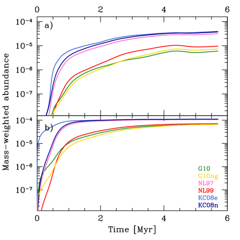
Figure 1: (a) Time evolution of the mass-weighted mean CO abundance in the simulations in set 1, representing the evolution of a low density cloud with mean hydrogen number density $n_{0}=100\>{\rm cm^{-3}}$. (b) As (a), but for the simulations in set 2, which model the evolution of a higher density cloud, with $n_{0}=300\>{\rm cm^{-3}}$.

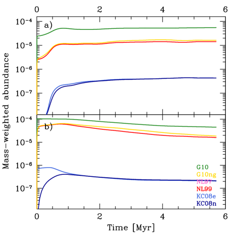
Figure 2: (a) Time evolution of the mass-weighted mean abundance of atomic carbon in the simulations in set 1, the low density cloud. Note that no line is plotted for the NL97 model, as this model does not track the abundance of atomic carbon. (b) As (a), but for the simulations in set 2.

In Figure 1a, we plot the evolution with time of the mass-weighted mean CO abundance, ${\langle x_{\rm CO}}\rangle_{\rm M}$, in the six simulations in set 1, our low density simulations. It is immediately obvious from this figure that the different methods do not agree on the amount of CO that is formed in the gas. Although there is good agreement between closely related models (e.g. KC08n and KC08e, or G10g and G10ng), there is roughly an order of magnitude difference in the CO fractions predicted by the full set of models. Furthermore, it is clear that the three simplest models (NL97, KC08e and KC08n) find a qualitatively different evolution for the mean CO abundance that the three more complex models (NL99, G10g and G10ng), predicting a more rapid rise in ${\langle x_{\rm CO}}\rangle_{\rm M}$ and a significantly larger final value.

The behaviour of ${\langle x_{\rm CO}}\rangle_{\rm M}$ in our higher density runs in set 2, illustrated in Figure 1b, further supports our finding that we can divide our models into two subsets that predict qualitatively different behaviour for the growth of the CO mass fraction. Runs NL97, KC08e and KC08n form almost all of their CO at $t<1\>{\rm Myr}$, and thereafter predict that ${\langle x_{\rm CO}}\rangle_{\rm M}$ should barely evolve. On the other hand, models NL99, G10g and G10ng find that CO forms over a more extended period, and predict that ${\langle x_{\rm CO}}\rangle_{\rm M}$ reaches a statistical steady state only at $t>5\>{\rm Myr}$. Runs NL97, KC08e and KC08n agree very well on the final amount of CO produced, predicting values for ${\langle x_{\rm CO}}\rangle_{\rm M}$ that differ by only a few percent. Runs NL99, G10g and G10ng also agree well at times $t>1\>{\rm Myr}$ on the amount of CO produced, but predict a final value for ${\langle x_{\rm CO}}\rangle_{\rm M}$ that is only 60% of the size of that predicted by runs NL97, KC08e and KC08n. The only difference between runs G10g and G10ng is the inclusion of grain-surface recombination in the former, and the good agreement between the CO distributions produced by these two models therefore indicates that the inclusion of this process has only a minor effect on the CO abundance. The good agreement between the results of these two models and the NL99 model is more of a surprise, and suggests that the composite species CH_x and OH_x in the NL99 model do a good job of reproducing the behaviour of the intermediate hydrocarbons and oxygen-bearing species that are tracked directly in models G10g and G10ng.

In Figure 2, we examine the evolution of the mass-weighted mean abundance of atomic carbon, ${\langle x_{\rm C}}\rangle_{\rm M}$, in our simulations. In this case, we compare only five models, as the NL97 chemical model does not contain atomic carbon, and so cannot make any prediction whatsoever about its abundance. It is immediately apparent from the Figure that there is a far larger degree of disagreement for the C abundances than for the CO abundances, particularly for our low density simulations. In these, we see three different evolutionary tracks. Run G10g forms a large amount of atomic carbon very quickly, reaching a value of ${\langle x_{\rm C}}\rangle_{\rm M}\sim 2\times 10^{-5}$ within only a few thousand years, an interval so short that it is not well represented in the Figure. Following this, the atomic carbon abundance continues to increase for the rest of the run, but at a much, much slower pace, reaching a final abundance ${\langle x_{\rm C}}\rangle_{\rm M}\sim 5.5\times 10^{-5}$ by the end of the simulation. In runs G10ng and NL99, there is also a rapid growth in the atomic carbon abundance at very early times, but in this case, this phase of rapid growth stops once ${\langle x_{\rm C}}\rangle_{\rm M}\sim 2\times 10^{-6}$. From this point until $t\sim 1\>{\rm Myr}$, the atomic carbon abundance continues to increase significantly, albeit at a much slower pace than at the very beginning of the simulation, while for $t>1\>{\rm Myr}$, there is little further evolution of ${\langle x_{\rm C}}\rangle_{\rm M}$. Finally, in runs KC08e and KC08n, the atomic carbon abundance does not display the very rapid growth at $t\ll 1\>{\rm Myr}$ seen in the other runs. Although there is significant growth in the atomic carbon abundance at $t<1\>{\rm Myr}$, the characteristic timescale is a significant fraction of a megayear, rather than the few thousand years found in the other models, and the amount of atomic carbon formed is much smaller. At $t>1\>{\rm Myr}$, there is a clear change in behaviour; the growth in ${\langle x_{\rm C}}\rangle_{\rm M}$ slows significantly, and it appears to have reached a steady-state by the end of the simulation. The final abundance of atomic carbon is considerably smaller than in the other runs: it is roughly a factor of thirty smaller than in than in runs G10ng or NL99, and more than a factor of 100 smaller than in run G10g.

In our higher density simulations, the size of the disagreement between run G10g and runs G10ng and NL99 is somewhat smaller, although significant differences remain. As in the lower density case, we see a very rapid growth in the atomic carbon abundance at very early times in these models, followed in this case by a slow decline as the atomic carbon is incorporated into CO molecules. The KC08e model also predicts a rapid rise in ${\langle x_{\rm C}}\rangle_{\rm M}$ followed by a slow decline, but the amount of atomic carbon produced in this model is a factor of 100 or so smaller than in the other models. Finally, model KC08n predicts a somewhat slower rise in ${\langle x_{\rm C}}\rangle_{\rm M}$ at early times, with a characteristic timescale of about 1 Myr, followed by a decline in the atomic carbon fraction at times $t>1\>{\rm Myr}$ that is almost indistinguishable from that in the KC08e model.

These discrepancies in the behaviour of the atomic carbon abundance in the various models are actually relatively easy to understand. In the KC08n and KC08e models, atomic carbon is produced only as an outcome of CO photodissociation, rather than directly from C⁺ by recombination. Since the formation rate of CO is relatively slow, relying as it does on a radiative association reaction, this means that the equilibrium abundance of atomic carbon is very small when the visual extinction is small. Therefore, in the KC08e model, the growth of the carbon abundance is regulated by the appearance of regions with high visual extinctions. In run 1, regions with a large enough visual extinction to allow for the production of non-negligible amounts of C and CO are created by the turbulent restructuring of the gas on a timescale of roughly $1\>{\rm Myr}$. In run 2, on the other hand, the higher mean density allows some regions to have a significant visual extinction (and hence a high equilibrium abundance of atomic carbon) even at $t=0$. In the KC08n model, the same consideration applies with regards to the dependence on visual extinction, but in addition, the growth of the atomic carbon abundance is also regulated by the time taken to form CO, which itself is of the order of $1\>{\rm Myr}$ or longer in much of the gas.

In the other three models, the most effective way to convert C⁺ to C is by direct recombination: gas-phase recombination in models G10ng and NL99, and a mix of gas-phase and grain-surface recombination in model G10g. The recombination time of fully ionized carbon in gas with $n=100\>{\rm cm^{-3}}$ and $T=60\>{\rm K}$ is roughly 0.2 Myr, assuming that the ionized carbon itself is the dominant source of the required electrons, and since the equilibrium C/C⁺ ratio at $t=0$ is much smaller than unity, it requires only a small fraction of a recombination time for the C/C⁺ ratio to reach its equilibrium value. Subsequent changes in the atomic carbon abundance are driven by two main effects: the restructuring of the gas by the turbulence, which puts more of the gas mass into dense, high $A_{\rm V}$ regions where the equilibrium C/C⁺ ratio is larger, and the conversion of C into CO in this same dense, well-shielded gas. This latter process is responsible for the fall-off in the atomic carbon abundance in the high density versions of runs G10g, G10ng and NL99 that occurs at $t>1\>{\rm Myr}$ (see Figure 2). The larger C/C⁺ ratio that we find in run G10g compared to runs G10ng and NL99 is an obvious consequence of the inclusion of grain-surface recombination, which is particularly effective when the ratio of the UV field strength $G_{0}$ to the mean density $n_{0}$ is small, as it is in our simulations.

Finally, we note that although it would be simple to investigate the evolution of the total mass of C⁺ in a similar fashion to our analysis of C and CO above, we have chosen to omit this, as in practice, C⁺, C and CO between them contain almost all of the available carbon in models G10g, G10ng and NL99 (and must contain 100% of it in the other models), and so there is nothing new to be learned from studying the time evolution of the C⁺.

5.2 Chemical abundances: dependence on density and visual extinction

We can gain more insight into the differences between the various models tested here by looking in more detail at their predictions for the distribution of CO at the end of the simulations. We know from previous work (Glover et al., 2010) that regardless of whether we examine them as a function of density or visual extinction, we always find considerable scatter in the CO abundances in a turbulent cloud. The reason for this is that the CO abundance is sensitive to both density and visual extinction, but these two quantities are only poorly correlated within turbulent clouds. Nevertheless, despite this scatter it can still be useful to examine averaged quantities, such as the total fraction of carbon represented by C⁺, C or CO, and how this varies as a function of density or visual extinction.

Therefore, in Figure 3, we show how the fraction of carbon in the form of C⁺, C or CO varies with density in the simulations. Let us focus initially on Figure 3a, which shows the results from the simulations in set 1. At densities below the mean density of $100\>{\rm cm^{-3}}$, all of the models predict that almost all of the carbon will be C⁺, and hence agree very well in their predictions of the C⁺ abundance. However, when we look at the abundances of C and CO at these low densities, we find substantial disagreement between the results of the different models. Let us start by considering the abundance of atomic carbon. This is entirely absent in the NL97 model, but represents 0.1% of the total carbon at $n=100\>{\rm cm^{-3}}$ in the KC08 models, roughly 1% in models G10ng and NL99, and closer to 10% in model G10g. The differences in the predictions for the atomic carbon abundance coming from various models persist over a wide range of densities, and at high densities, where atomic carbon is abundant, they also cause significant differences in the C⁺ fraction, which, for instance, falls off more rapidly with increasing density in run G10g than in the other runs. Turning to the CO fraction, we find that runs G10g, G10ng and NL99 agree well with each other on the behaviour of the CO fraction, as do runs NL97, KC08e and KC08n, but that there is a significant difference in the behaviour of these two sets of runs. All of the models predict a sharp rise in the CO fraction with increasing number density, and agree that the fraction of carbon in CO should be close to 100% for number densities of order $10^{4}\>{\rm cm^{-3}}$. However, at densities below $10^{4}\>{\rm cm^{-3}}$, we find that the CO fraction in runs NL97, KC08e and KC08n is systematically larger than in the other three runs. For example, at $n=1000\>{\rm cm^{-3}}$, the three simple models predict a CO fraction of roughly 80–90%, while runs G10g, G10ng, and NL99 predict a value that is closer to 10%.

In Figure 3b, which shows the behaviour of the simulations in set 2, we find very similar results. In this case, the transition from C⁺ to C to CO takes place over a wider range of densities, and the gas becomes CO dominated at a lower density than before. This is a consequence of the higher mean extinction of the gas – in these simulations, there is more gas at all densities that is well shielded from the UV background and hence can maintain a high CO abundance. Nevertheless, the qualitative behaviour of the CO fraction as a function of density remains the same as in our lower density runs. Models NL97, KC08e and KC08n continue to agree well over the whole range of densities plotted, as do models G10g, G10ng and NL99, with the first set of models predicting systematically higher CO fractions than the second set. At $n>5000\>{\rm cm^{-3}}$, all six models agree that the gas should be completely CO-dominated.

In Figure 4, we show how the fraction of carbon in the form of C⁺, C or CO varies as a function of the effective visual extinction, defined for any given cell in our simulations as

$$A_{\rm V,eff}=-\frac{1}{2.5}\ln\left[\frac{1}{6}\left(\sum_{p=1}^{3}e^{-2.5A_{\rm V}(x_{p+})}+e^{-2.5A_{\rm V}(x_{p-})}\right)\right]$$ (18)

where $A_{\rm V}(x_{p+})$ is the visual extinction of material between that cell and the edge of the volume in the positive direction along the $x_{p}$ axis, and so forth. The choice of the factor of 2.5 occurs because in our models, the CO photodissociation rate scales with the visual extinction $A_{\rm V}$ as $\exp(-2.5A_{\rm V})$. The value of $A_{\rm V,eff}$ defined in this fashion corresponds to the visual extinction used in our code, in the context of our six-ray approximation, for computing the CO photodissociation rate.

Figure 4 displays a number of familiar features. Models G10g, G10ng and NL99 all agree well on the evolution of the CO fraction with increasing visual extinction, just as they did on its evolution with increasing density. Models G10ng and NL99 also agree on the behaviour of the C and C⁺ fractions at all but the highest visual extinctions, while model G10g predicts a much larger atomic carbon fraction at $A_{\rm V,eff}\sim 1$–2 than in the other two models, and hence a correspondingly smaller C⁺ fraction. Models NL97, KC08e and KC08n agree well with each other regarding the CO fraction, but produce more CO at low visual extinctions than the other three runs.

Figure 4b also displays a curious feature in the plot of the atomic carbon fraction at very low $A_{\rm V,eff}$ in runs G10g, G10ng and NL99. Below an effective visual extinction of roughly 0.4, the atomic carbon fraction increases with decreasing $A_{\rm V,eff}$ in these three runs. However, further investigation shows that this feature is a numerical artifact related to our use of the six-ray approximation. As previously discussed in Glover et al. (2010), the effective visual extinction of material right at the edge of the computational volume is higher than it should be, owing to the poor angular sampling of the radiation field, and in practice only few zones very close to the edge have effective visual extinctions $A_{\rm V,eff}<0.5$. Because of this, when we compute the mass fractions for $A_{\rm V,eff}<0.5$, we are averaging over only a small number of zones, and hence are far more sensitive to the effects of outliers than we would be at higher $A_{\rm V,eff}$. In this particular case, the anomalous behaviour of the atomic carbon fraction is due to the contribution from a small clump of dense gas located at the edge of the simulation volume. The higher density of this gas enables C⁺ recombination to be more effective, and allows it to have a higher atomic carbon abundance than the rest of the gas at this visual extinction. The effect is more pronounced in run G10g because of the inclusion of grain-surface recombination in that model.

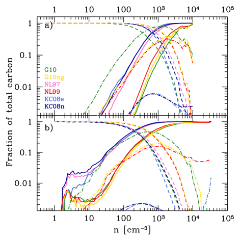
Figure 3: (a) Fraction of the total available carbon found in the form of C⁺ (dashed lines), C (dash-dotted lines), or CO (solid lines) in the simulations in set 1, plotted as a function of density. Note that as model NL97 does not include atomic carbon, no line is plotted in this case. (b) As (a), but for the simulations in set 2.

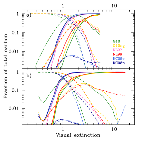
Figure 4: (a) As Figure 3a, but showing the variation in the C⁺, C and CO fractions as a function of visual extinction $A_{\rm V}$ for the simulations in set 1. (b) As (a), but for the simulations in set 2.

5.3 CO column densities and integrated intensities

Although informative, the quantities that we have examined so far have the significant disadvantage that they are not observable in real molecular clouds. It is therefore useful to examine whether the differences between the models that we have already discussed will lead to clear differences in the observable properties of the CO distribution.

We begin by examining the behaviour of the CO column density distribution. CO column densities are directly observable in the ISM along low extinction ($A_{\rm V}\sim 2$ or less) sightlines to bright background stars, where they can be accurately determined by UV absorption measurements (see e.g. Sheffer et al., 2007). For higher extinctions, this technique is no longer effective, and one typically relies on CO emission, which is an accurate tracer of the CO column density only for transitions which are optically thin and uniformly excited (see e.g. Pineda, Caselli & Goodman, 2008; Shetty et al., 2011). Since much of the ¹²CO emission coming from Galactic GMCs is optically thick, information on the CO column density distributions in these clouds generally comes from observations of rarer CO isotopologues such as ¹³CO or C¹⁸O, which are optically thin over a much wider range of cloud column densities.

The probability density functions (PDFs) for the CO column density in our two sets of runs are plotted in Figure 5. In our low density runs, we see that the PDFs are relatively flat, indicative of there being a roughly equal probability of selecting any particular CO column density within a relatively wide range. This is quite unlike the PDF of total column density, which has the characteristic log-normal shape ubiquitously found in simulations of supersonic turbulence (see e.g. Ostriker, Stone & Gammie, 2001), and demonstrates that the CO is not a particularly accurate tracer of the underlying density distribution in our low density simulations (see also Shetty et al., 2011, for more on this point). In runs NL97, KC08e and KC08n, we begin to see the influence of this underlying structure between CO column densities of $10^{17}\>{\rm cm^{-2}}$ and a few times $10^{18}\>{\rm cm^{-2}}$, where there is a clear peak in the PDF, but no such feature is visible in the CO column density distributions produced in the other three runs. In our higher density runs, on the other hand, the influence of the underlying density structure of the gas is far more pronounced, with all of the runs showing a clear peak in the PDF at high CO column densities. The PDFs can best be understood as the superposition of two different features: a log-normal portion at high $N_{\rm CO}$, corresponding to lines of sight along which most of the carbon is in molecular form, leading to a CO column density that simply traces the total column density, and an extended tail at much lower $N_{\rm CO}$ that corresponds to lines of sight along which the CO is significantly photodissociated.

Comparing the predictions of the different models, we see that once again the runs can be separated into two distinct sets. Runs G10g, G10ng and NL99 agree reasonably well with each other, particularly for the higher density cloud, but produce results that differ significantly from those found in runs NL97, KC08e and KC08n. The latter models produce narrower CO column density PDFs, with a more pronounced peak at high $N_{\rm CO}$, and with much smaller probabilities at low $N_{\rm CO}$. One consequence of this is that the CO is a better tracer of the underlying density distribution in runs NL97, KC08e and KC08n than in runs G10g, G10ng and NL99.

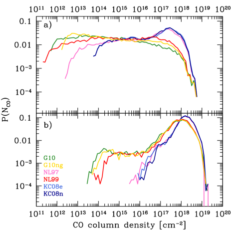
Figure 5: (a) CO column density PDFs for the runs in set 1. (b) As (a), but for the runs in set 2.

We have also computed estimates of the frequency-integrated intensities of the $J=1\rightarrow 0$ line of CO corresponding to these CO column densities, using the same technique as in Glover & Mac Low (2011). To briefly summarize, we assume that the CO is in local thermodynamic equilibrium (LTE), and is isothermal, with a temperature equal to a weighted mean temperature for the gas, computed using the CO number density as the weighting function:

$$T_{\rm mean,CO}=\frac{\sum_{i,j,k}T(i,j,k)n_{\rm CO}(i,j,k)}{\sum_{i,j,k}n_{\rm CO}(i,j,k)},$$ (19)

where we sum over all grid zones $i,j,k$. We also assume that the CO linewidth is uniform, and is given by $\Delta v=3\>{\rm km}\>{\rm s^{-1}}$ (which is roughly equal to the one-dimensional velocity dispersion we would expect to find in a gas with an RMS turbulent velocity of $5\>{\rm km\>s^{-1}}$). Given these assumptions, we can relate the CO column density to the optical depth in the $J=1\rightarrow 0$ line using (Tielens, 2005)

$$\tau_{10}=\frac{A_{10}c^{3}}{8\pi\nu_{10}^{3}}\frac{g_{1}}{g_{0}}f_{0}\left[1-\exp\left(\frac{-E_{10}}{kT}\right)\right]\frac{N_{\rm CO}}{\Delta v},$$ (20)

where $A_{10}$ is the spontaneous radiative transition rate for the $J=1\rightarrow 0$ transition, $\nu_{10}$ is the frequency of the transition, $E_{10}=h\nu_{10}$ is the corresponding energy, $g_{0}$ and $g_{1}$ are the statistical weights of the $J=0$ and $J=1$ levels, respectively, and $f_{0}$ is the fractional level population of the $J=0$ level. We can then convert from $\tau_{10}$ to the integrated intensity, $W_{\rm CO}$, using the same curve of growth analysis as in Pineda, Caselli & Goodman (2008):

$$W_{\rm CO}=T_{\rm b}\Delta v\int_{0}^{\tau_{10}}2\beta(\tilde{\tau}){\rm d}\tilde{\tau},$$ (21)

where $T_{\rm b}$ is the brightness temperature of the line, which we assume is simply equal to $T_{\rm mean,CO}$, and $\beta$ is the photon escape probability, given by

$$\beta(\tau)=\left\{\begin{array}[]{lr}[1-\exp(-2.34\tau)]/4.68\tau&\tau\leq 7,\\ \left(4\tau\left[\ln\left(\tau/\sqrt{\pi}\right)\right]^{1/2}\right)^{-1}&\tau>7.\end{array}\right.$$ (22)

Although the estimates of $W_{\rm CO}$ generated by this procedure are probably accurate to within only a factor of a few, this level of accuracy is sufficient for our purpose here.

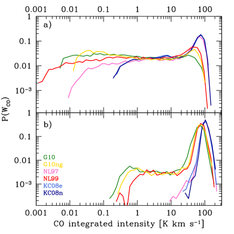
Figure 6: (a) PDF of the integrated intensity in the $J=1\rightarrow 0$ line of ¹²CO in the runs in set 1. The integrated intensities are estimates, calculated using the technique described in Glover & Mac Low (2011) and summarized in Section 5.3. (b) As (a), but for the runs in set 2.

In Figure 6, we plot PDFs of integrated intensity for the simulations. At $W_{\rm CO}<30{\rm K\>km\>s^{-1}}$, these PDFs closely resemble the CO column density PDFs, while at higher integrated intensities, we see a clear peak in the PDF even when there is no corresponding feature in the CO column density distribution at high $N_{\rm CO}$. This behaviour can be easily understood as being due to the change from having optically thin CO emission at $W_{\rm CO}\sim 30{\rm K\>km\>s^{-1}}$ and below, to having optically thick emission at higher $W_{\rm CO}$. In the optically thin regime, $W_{\rm CO}\propto N_{\rm CO}$, and so we see similar behaviour in both PDFs. In the optically thick regime, on the other hand, $W_{\rm CO}$ increases only slowly with increasing $N_{\rm CO}$, and so we find a ‘pile-up’ of values at these intensities (see also the more detailed discussion of this effect in Shetty et al., 2011).

5.4 The C/CO ratio

Another potentially useful quantity for distinguishing between different models is the ratio of the column density of atomic carbon to that of CO. A number of groups have attempted to measure this value (see e.g. Ingalls et al., 1997; Ikeda et al., 2002; Bensch et al., 2003), typically finding values in the range of 0.1 to 3, with the higher values coming from lower column density translucent clouds, and the lower values coming from higher column density dark clouds. Although a comprehensive comparison between our results and these observational determinations is outside of the scope of our current paper, a simple comparison nevertheless proves illuminating.

In Table 3, we list the ratio of the mean column density of atomic carbon, $\bar{N}_{\rm C}$, to the mean column density of CO, $\bar{N}_{\rm CO}$, that we obtain for each of our runs, with the exception of the two NL97 models, which do not track atomic carbon. We see that two of the models – G10ng and NL99 – produce values for the C/CO column density ratio that are broadly in line with the values observed in real clouds. On the other hand, model G10g in run 1 produces a significantly higher value than is observed, suggesting that our treatment of C⁺ recombination on grains may actually overestimate the rate at which this process occurs in the real ISM. In this context, it is interesting to note a recent study by Liszt (2011) that also finds indications that we do not currently understand the role that grain-surface recombination of C⁺ plays in the transition from C⁺ to C to CO. Finally, we see from Table 3 that the KC08e and KC08n models produce significantly smaller C/CO ratios than are seen in real clouds, likely because these models neglect the effect of gas-phase recombination of C⁺.

Table 3: Comparison of C/CO column density ratios

Method	$\bar{N}_{\rm C}/\bar{N}_{\rm CO}$
	Run 1	Run 2
G10g	9.3	0.68
G10ng	2.2	0.28
NL99	1.5	0.23
KC08e	0.01	0.002
KC08n	0.01	0.002

5.5 The CO-to-H₂ conversion factor

Before we conclude our study of the details of the CO distribution in our simulations, it is interesting to examine whether the differences in the amount of CO formed in the various runs, and in its spatial distribution, lead to significant differences in the CO-to-H₂ conversion factor, $X_{\rm CO}$. This is conventionally defined as the ratio of the H₂ column density to the integrated intensity of the $J=1\rightarrow 0$ transition of CO, i.e.

$$X_{\rm CO}=\frac{N_{\rm H_{2}}}{W_{\rm CO}}.$$ (23)

Observations of Galactic GMCs show that $X_{\rm CO}$ appears to be roughly constant from cloud to cloud, with a mean value of $X_{\rm CO}=2\times 10^{20}{\rm cm^{-2}\>K^{-1}\>km^{-1}\>s}$ (see e.g. Dame et al., 2001), and in Glover & Mac Low (2011) we showed that our turbulent cloud models reproduce this behaviour, provided that the mean visual extinction of the clouds exceeds a threshold value of $A_{\rm V}\sim 2$–3.

To estimate $X_{\rm CO}$ for the simulations considered in this paper, we start by finding the mean of the distribution of integrated intensities that we have already computed for each simulation. Armed with a mean integrated intensity for each simulation, we next compute the mean H₂ column density for each simulation, following which we can obtain our estimate of $X_{\rm CO}$ simply by taking the ratio of these two mean quantities. The values obtained using this procedure are listed in Table 4.

In the low density case, models NL97, KC08e and KC08n yield values for $X_{\rm CO}$ that are a factor of a few smaller than the standard Galactic value, while the other three runs yield values that are in much better agreement with the observations. However, given that our estimates of $X_{\rm CO}$ here are likely only accurate to within a factor of a few, it is unclear whether the difference between predictions of the NL97, KC08e and KC08n models and the observations is really meaningful. In any case, in the high density case we find much better agreement between the models, with all of them now producing values that are somewhat smaller than the Galactic value. The reason for this similarity is that all of the runs agree reasonably well (to within a factor of two) on the peak value of the integrated CO intensity found in the simulation, with the significant differences in the $W_{\rm CO}$ distribution occurring for values considerably below the peak. Our estimate of $X_{\rm CO}$ is dominated by the contribution of lines of sight with integrated intensities close to the peak value, and is insensitive to the behaviour of lines of sight with low $W_{\rm CO}$, and so this diagnostic tells us little about the low intensity sightlines.

Table 4: Comparison of the CO-to-H₂ conversion factor, $X_{\rm CO}$, at the end of the runs

Method	$X_{\rm CO}$ [$10^{20}\>{\rm cm^{-2}}\>({\rm K\>km\>s^{-1}})^{-1}$]
	Run 1	Run 2
G10g	2.67	1.30
G10ng	2.01	1.23
NL97	0.57	0.90
NL99	1.47	1.17
KC08e	0.50	0.89
KC08n	0.49	0.87

5.6 Gas temperature

C⁺, C and CO are all important coolants at the temperatures and densities found within molecular clouds, and so differences in the predicted distributions of these species may have an effect on the thermal evolution of the gas and on its temperature structure at the end of the simulation.

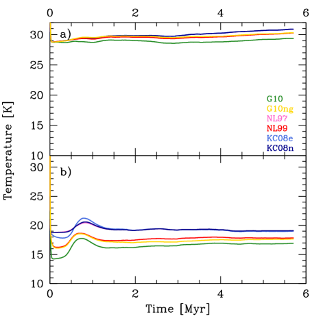
Figure 7: (a) Time evolution of the mass-weighted mean gas temperature in the simulations in set 1. (b) As (a), but for the simulations in set 2.

We have investigated this by examining the time evolution of the mass-weighted mean gas temperature, plotted in Figure 7. In the low density runs, the mean temperature drops very rapidly from our initial value of 60 K to a value of approximately 30 K. Thereafter, it evolves very little over the course of the simulation. The six different chemical models predict very similar values for the mean temperature. The most discrepant outcome is for model G10g, which predicts a final mean temperature that is roughly 1 K cooler than in the other runs. This result is easy to understand given the results for the mean mass-weighted abundances of C⁺, C and CO in these runs, discussed earlier in Section 5.1. C⁺ is the dominant form of carbon in all of these runs, and hence will be the dominant coolant. Differences in the abundances of C or CO will therefore have only a minor impact on the energy balance of the gas, and hence will have little effect on the mean gas temperature. However, in the case of model G10g, the atomic carbon abundance becomes large enough that its contribution to the cooling of the gas can no longer be neglected. Since the energy separation of the fine structure levels in neutral carbon is significantly smaller than in singly ionized carbon, the former is a more effective low temperature coolant than the latter, and so increasing the C abundance at the expense of the C⁺ abundance leads to an overall lower temperature for the gas.

In the higher density runs, the mean temperature again drops very rapidly initially, before stabilizing at a value of around 17–19 K. In this case, the difference between the models is more pronounced, with runs NL97, KC08 and KC08n predicting the highest temperatures, and run G10g predicting the lowest. However, at the end of the simulations, the difference between the runs is only 2 K, or roughly 10%. The differences can again be easily understood on the basis of our prior results for the mean abundances. In this case, the C and CO abundances are much higher, and so C⁺ is no longer the dominant radiative coolant. Instead, the cooling is typically dominated by CO (runs NL97, KC08e and KC08n) or by a mixture of atomic carbon and CO (the other three runs). There is a clear inverse correlation between the amount of atomic carbon present in the gas and the final mean temperature.

We have also examined the temperature distribution of the gas at the end of the simulations, as shown in Figure 8, where we plot mass-weighted PDFs of the gas temperature for the various runs. In both the low and the high density cases, the PDF at $T>30\>{\rm K}$ shows almost no dependence on the chemical model, consistent with it representing gas which is dominated by C⁺ in all of the models. Below 30 K, however, clear differences become apparent. In the low density case, runs G10ng, NL99, KC08n, KC08e and NL97 all show a clear peak at a temperature of around 20 K, but in run G10g, this peak occurs at the lower temperature of 10 K. Runs NL97, KC08e and KC08n all produce very little gas cooler than 10 K, but in the other three runs we find a significant fraction of gas with temperatures in the range of 5–10 K. In the high density run, the behaviour changes slightly. Runs NL97, KC08e and KC08n still have a clear feature in the PDF at $T\sim 20\>{\rm K}$, but the true peak is now found at a temperature slightly larger than 10 K. In runs G10g, G10ng and NL99, on the other hand, the peak is at the slightly lower temperature of 9 K, with this feature being more pronounced in run G10g than in the other two runs. The behaviour of these three runs at temperatures below this peak value is very similar.

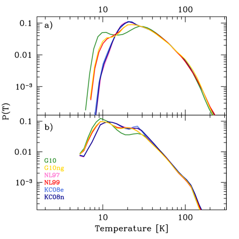
Figure 8: (a) Mass-weighted temperature PDF for run 1. (b) As (a), but for run 2. Note that in both cases, the results for the NL97 and KC08e runs are barely distinguishable from those for the KC08n run.

The differences between the low temperature behaviour in the various runs can be relatively easily understood. In the low density runs, little CO is formed, and so in most of the gas, the dominant cooling mechanisms are C⁺ and C fine structure emission, with some contribution from dust in the densest regions. The energy separation of the ²P_1/2 ground state and the ²P_3/2 excited state of C⁺ is approximately 92 K, and hence it cannot easily cool the gas below about 15–20 K, owing to the exponential suppression of the cooling rate. On the other hand, atomic carbon has a separation of only 24 K between its two lowest lying energy levels, and so remains an effective coolant down to temperatures of order 5 K. Therefore, chemical models producing greater quantities of atomic carbon will tend to produce lower gas temperatures. For instance, as we have already seen, run G10g produces more atomic carbon in intermediate density gas ($n\sim 1000\>{\rm cm^{-3}}$) than runs G10ng or NL99. In the low density case, little CO is formed, as we have already seen, and so most of the 10 K gas produced in this case comes from regions that are dominated by cooling from neutral carbon. Consequently, run G10g produces significantly more of this 10 K gas than runs G10ng or NL99. On the other hand, run NL97 produces no neutral carbon, and hence only very little 10 K gas. In the higher density simulations, which have much higher mean CO abundances, much more of the 10 K gas is situated in regions dominated by CO cooling, and so the differences between runs G10g, G10ng and NL99 are much smaller than in the low density case. The lack of neutral carbon in run NL97, and the fact that it underproduces CO at low densities mean that it still disagrees with these three models, and produces less very cold gas. The behaviour of runs KC08e and KC08n is very similar to that of run NL97 because the small amount of neutral carbon produced in runs KC08e and KC08n is not enough to significantly affect the thermal balance of the gas, and as we have already seen, the CO and C⁺ abundances in these runs are very similar to those in run NL97.

5.7 Gas density

Finally, we have investigated whether the differences in the temperature distributions examined above lead to any significant differences in the density distribution of the gas, as quantified by the density PDF. This is of particular importance for understanding the level of accuracy in the modelling of the CO chemistry that is necessary in order to allow us to model star formation accurately, as there are a number of theoretical models that argue that it is the shape of the density PDF that determines the stellar initial mass function (Padoan, Nordlund & Jones, 1997; Padoan & Nordlund, 2002; Hennebelle & Chabrier, 2008, 2009) or the star formation rate (Krumholz & McKee, 2005; Padoan & Nordlund, 2011) in a molecular cloud.

In Figure 9a, we plot the density PDFs for the simulations in set 1. In Figure 9b, we show a similar plot for the simulations in set 2. We see that in both cases, over most of the density range spanned by the PDF, there is essentially no difference between the results of any of the runs, indicating that at these densities, the physical structure of the gas is insensitive to the CO abundance. Minor differences start to become apparent in the high density tail of the PDFs, but even here the differences are small. In addition, they occur at densities that are not well resolved in our current simulations, and we cannot be completely certain that they would persist in higher resolution simulations.

Figure 9: (a) Mass-weighted density PDF for the runs in set run 1. Minor differences are apparent in the high density tail, at $n>5000\>{\rm cm^{-3}}$, but over the rest of the density range, all six runs agree very well. (b) As (a), but for the runs in set 2. Again, there is very good agreement between the runs at almost all densities, with only a few minor differences becoming apparent in the high density tail.

Padoan, Nordlund & Jones (1997) presented results indicative of a relationship between the dispersion $\sigma_{s}$ of the logarithmic density contrast $s=\ln(\rho/\rho_{0})$ (where $\rho_{0}$ is the mean gas density), and the volume-weighted RMS Mach number ${\cal M}$, finding that

$$\sigma_{s}^{2}=\ln\left(1+b^{2}{\cal M}^{2}\right),$$ (24)

with $b\simeq 0.5$. Recent work by Federrath, Klessen & Schmidt (2008) has shown that the proportionality parameter $b$ is sensitive to the relative strength of the solenoidal and compressive modes in the forcing field used to drive the turbulence, and ranges from $b\sim 1/3$ for purely solenoidal forcing to $b\sim 1$ for purely compressive forcing. In each case, the effects of the gas temperature enter through the dependence of $\sigma_{s}$ on the volume-weighted RMS Mach number. In our simulations, the dominant contributions to ${\cal M}$ come from low density, warm gas that is dominated by C⁺ cooling. The differences in the temperature distribution of the cold, denser material have little influence on ${\cal M}$. We find that ${\cal M}$ varies by no more than 1–2% from run to run in both the low density and high density cases, thereby explaining why we see so little variation in the density PDF from run to run.

6 Discussion

6.1 Understanding the differences in CO production

Our comparisons in the previous section have demonstrated that the G10g, G10ng and NL99 models agree very well regarding the time evolution of the CO abundance and the spatial distribution of the CO. The most significant difference between the treatment of the carbon chemistry in these three models turns out to be the inclusion of grain-surface recombination in model G10g, or more specifically, the recombination of C⁺ ions on grain surfaces. The inclusion of this process has a significant effect on the ratio of C⁺ to C in the gas, and therefore indirectly affects the temperature distribution, since C is a much more effective coolant than C⁺ at gas temperatures below 20 K.

The KC08e, KC08n and NL97 models also agree well with each other, but disagree with the G10g, G10ng and NL99 models in two major respects. First, they predict a shorter formation timescale for the CO, particularly in the high density run. Second, they predict systematically larger values for the CO fraction as a function of density or visual extinction. Both of these disagreements between the two sets of models result from the same underlying cause. In the KC08e, KC08n and NL97 models, the rate-limiting step in the formation of CO is the initial radiative association between C⁺ and H₂, a reaction that has a rate coefficient $k_{0}=5\times 10^{-16}\>{\rm cm^{3}}\>{\rm s^{-1}}$ in the NL97 model, and a similar value in the other two models. The rate per unit volume at which CH${}_{2}^{+}$ ions (or CH_x radicals) form in this model is therefore given by

$$R_{1}=5\times 10^{-16}n_{\rm C^{+}}n_{\rm H_{2}}.$$ (25)

In the G10g, G10ng and NL99 models, on the other hand, there are multiple routes leading to the formation of CO and hence the situation is somewhat more complicated. In practice, the main contributions come from two main reactions pathways, one initiated by the radiative association of C⁺ with H₂, as above, and a second initiated by the reaction of atomic carbon with H${}_{3}^{+}$. The latter reaction occurs rapidly, and the rate-limiting step for this second reaction pathway is hence not the reaction between C and H${}_{3}^{+}$, but rather the formation of the H${}_{3}^{+}$ ion itself. This occurs as a consequence of the cosmic ray ionization of H₂, which yields H${}_{2}^{+}$ ions that then rapidly react with H₂ to form H${}_{3}^{+}$:

$${\rm H_{2}^{+}}+{\rm H_{2}}\rightarrow{\rm H_{3}^{+}}+{\rm H}.$$ (26)

In regions where at least a few percent of the carbon is ionized, the free electron abundance is roughly equal to the abundance of ionized carbon, and the dominant destruction mechanism for the H${}_{3}^{+}$ ions is dissociative recombination:

$${\rm H_{3}^{+}}+{\rm e} \rightarrow {\rm H_{2}}+{\rm H},$$ (27)

$$\rightarrow {\rm H}+{\rm H}+{\rm H}.$$ (28)

In these conditions, the net rate at which CH${}_{2}^{+}$ ions are produced by reactions between C and H${}_{3}^{+}$ is therefore given by

$$R_{2}=2\zeta_{\rm H}n_{\rm H_{2}}\frac{k_{\rm CH_{2}^{+}}}{k_{\rm dr}}\frac{n_{\rm C}}{n_{\rm C^{+}}},$$ (29)

where $\zeta_{\rm H}$ is the cosmic ray ionization rate of atomic hydrogen, $k_{\rm dr}$ is the rate coefficient for the dissociative recombination of H${}_{3}^{+}$ ions and $k_{\rm CH_{2}^{+}}$ is the rate coefficient for the reaction

$${\rm C+H_{3}^{+}\rightarrow CH_{2}^{+}+H}.$$ (30)

In cold gas, $k_{\rm CH_{2}^{+}}/k_{\rm dr}\simeq 0.01$, and hence

$$R_{2}\simeq 2\times 10^{-19}\zeta_{\rm H,17}\,n_{\rm H_{2}}\frac{n_{\rm C}}{n_{\rm C^{+}}},$$ (31)

where $\zeta_{\rm H,17}=\zeta_{\rm H}/10^{-17}\>{\rm s^{-1}}$. (Recall that in our simulations, $\zeta_{\rm H,17}=1$). The net rate of formation of CH${}_{2}^{+}$ ions in models G10g, G10ng and NL99 is approximately equal to $R_{1}+R_{2}$, since other processes make only minor contributions, while in models NL97, KC08e and KC08n, the rate of formation of CH${}_{2}^{+}$ ions is simply $R_{1}$. Note, however, that since $R_{1}$ depends on $n_{\rm C^{+}}$, which is generally larger in models NL97, KC08e and KC08n than in the other models, the size of the rate $R_{1}$ in the simple models is generally larger than in the more complex models. To avoid confusion, it is useful to distinguish between these two cases by writing the rate in the simple models (NL97, KC08e, KC08n) as $R_{\rm 1,s}$ and writing the rate in the more complex models (NL99, G10ng, G10g) as $R_{\rm 1,c}$.

We next consider the conditions in which the rate of CH${}_{2}^{+}$ formation in the complex models, given by $R_{\rm 1,c}+R_{2}$, is bigger than the rate in the simple models, given by $R_{\rm 1,s}$. Starting with the inequality,

$$R_{\rm 1,c}+R_{2}>R_{\rm 1,s},$$ (32)

we can subtract $R_{\rm 1,c}$ from both sides, giving us

$$R_{2}>(R_{\rm 1,s}-R_{\rm 1,c}).$$ (33)

If we denote the number density of C⁺ in the simple models as $n_{\rm C^{+},s}$, and denote the same quantity in the complex models as $n_{\rm C^{+},c}$, then we can write this inequality as

$$2\times 10^{-19}\zeta_{\rm H,17}\,n_{\rm H_{2}}\frac{n_{\rm C}}{n_{\rm C^{+},c}}>5\times 10^{-16}n_{\rm H_{2}}(n_{\rm C^{+},s}-n_{\rm C^{+},c})$$ (34)

where we have assumed that the H₂ abundance is the same in both cases. If the CO abundance is small compared to the abundances of C⁺ and/or C, then in the simple models, the number density of C⁺ ions will be roughly equal to the number density of carbon atoms in all forms, i.e. $n_{\rm C^{+},s}\simeq n_{\rm C,tot}$. In the complex models, on the other hand, we have $n_{\rm C^{+},c}+n_{\rm C}\simeq n_{\rm C,tot}$, and hence in these conditions $n_{\rm C^{+},s}-n_{\rm C^{+},c}\simeq n_{\rm C}$. We can use this fact to simplify Equation 34, which reduces to the following constraint on $n_{\rm C^{+},c}$:

$$n_{\rm C^{+},c}<4\times 10^{-4}\zeta_{\rm H,17}.$$ (35)

In practice, this inequality is rarely satisfied in the gas in our simulations. For example, in solar metallicity gas with $n=300\>{\rm cm^{-3}}$, it is satisfied only when the ratio of atomic to ionized carbon is of the order of a thousand to one. Therefore, in general, the rate at which CH${}_{2}^{+}$ ions are produced in the more complex models is slower than the rate at which they are produced in the simpler models.

This fact explains most of the difference that we see between our two sets of chemical models. When $n_{\rm C^{+}}\gg n_{\rm C}$, all of the models produce CH${}_{2}^{+}$ ions (and hence also CO molecules) at a very similar rate. In models G10g, G10ng and NL99, however, the physical conditions that allow large CO fractions to be produced (high density and high visual extinction) also allow the recombination of C⁺ to be far more effective than the photoionization of atomic carbon, meaning that the equilibrium ratio of C to C⁺ in these regions strongly favours atomic carbon. As the carbon recombines (which occurs on a timescale that is short compared to the CO formation timescale), the CO formation rate decreases for the reasons outlined above. The same effect does not occur in the NL97, KC08e or KC08n models because none of these models include the effects of C⁺ recombination: model NL97 ignores atomic carbon entirely, while in models KC08e and KC08n, it is produced only by the photodissociation of CO. Therefore, the CO formation rate in models NL97, KC08e or KC08n is in general larger than in models G10g, G10ng and NL99, explaining the shorter CO formation timescales and larger CO fractions we find in the former models with respect to the latter.

7 Conclusions

In this paper, we have examined several different approaches to modelling the chemistry of CO in three-dimensional numerical simulations of turbulent molecular clouds. The simplest approaches (NL97, KC08n, KC08e) include only a very small number of reactions and reactants, with the KC08e model making the additional simplifying assumption of chemical equilibrium. The NL99 adds a number of additional reactions and reactants, but still remains relatively simple, owing to its use of artifical species (CH_x, OH_x) as stand-ins for a much wider range of real molecular ions, radicals and molecules. Finally, the most complex models examined here (G10g and G10ng) add a few more non-equilibrium reactants, a large number of additional reactants that are assumed to be in chemical equilibrium, and a large number of additional reactions. The complexity of these two models lies close to the upper limit of what is practical to include in a three-dimensional simulation at present, but still represents a significant simplification when compared with state-of-the-art one-zone or one-dimensional chemical models (see e.g. the PDR codes discussed in Röllig et al. 2007).

As one would expect, the simpler one makes the chemical model, the faster it becomes to compute the chemical evolution of the gas. Models NL97, KC08e and KC08n allow the simulations to run roughly an order of magnitude faster than the reference model, while model NL99 yields a runtime three times longer than the simple models, but still three to four times shorter than the models based on Glover et al. (2010).

Looking in more detail at the results of the simple networks, we find that they tend to produce more CO than the more complex networks, for the reasons outlined in the previous section. It is also clear that one area in which the simpler models fall down is in their treatment of atomic carbon. This is ignored entirely in the NL97 model, and is significantly underproduced in the KC08e and KC08n models, owing to the omission of the effects of C⁺ recombination from these models. It should however be noted that the Keto & Caselli (2008) chemical model was designed for use in a study of the thermal balance of prestellar cores with mean densities that are more than an order of magnitude larger than the mean densities considered in our simulations. In these conditions, the gas is CO-dominated, atomic carbon is not an important coolant, and the Keto & Caselli (2008) model does a good job of capturing the essential physics of the gas. It performs more poorly in our study only because we are applying it to a range of physical conditions outside of those for which it was designed.

Turning our attention to the more complex networks, we find that models NL99 and G10ng produce very similar results in all of our comparisons, and that the differences between the results of these models and that of model G10g are easily understandable as consequences of the inclusion of grain-surface recombination of C⁺ in the latter, which significantly affects the relative abundances of C and C⁺ produced in the gas. We also note that the inclusion of this process leads to a significant overproduction of atomic carbon and hence yields values for the C/CO ratio that are significantly higher than those observed in real molecular clouds. Models NL99 and G10ng, on the other hand, yield values for the C/CO ratio that appear to be consistent with observations.

Given that model NL99 produces very similar values to model G10ng for the C and CO abundances, but in only one-third of the computational time, we suggest that the former is a better choice than the latter if one is primarily interested in the C⁺ to C to CO transition, or in the details of the resulting CO distribution. On the other hand, the more complex G10ng model is a better choice if one is also interested in the distributions of species not tracked in the NL99 model, such as CH, CH⁺, OH, H₂O or O₂, and is willing to pay the additional computational cost for tracking these species. Furthermore, if all one is interested in is an approximate picture of which regions are likely to have high CO abundances (as may be of interest in a large-scale simulation of the Galactic ISM, such as Dobbs et al. 2008), then any of these models are likely to do a reasonable job, as the differences between the CO distributions that they predict are not enormous and are likely smaller than the uncertainties introduced by the inevitably limited resolution possible within large-scale simulations. For this kind of modelling, it would therefore make sense to choose one of the simpler, faster models, such as NL97, KC08e or KC08n.

Finally, we have examined the effects of the choice of chemical network on the density and temperature distributions in our model clouds. We find that the influence of the chemistry is surprisingly limited. In both the low and the high density model clouds, much of the cloud volume is filled with warm gas ($T>30\>{\rm K}$). Most of the carbon in this warm material is in the form of C⁺, and hence C⁺ cooling dominates. All of the chemical networks that we examined do a good job of representing this material. The chemistry of the gas plays a significant role in determining the temperature only if one looks at colder, denser gas, with much higher C and CO fractions, but even here, changing the chemistry changes the gas temperatures by at most a factor of two. These small temperature changes have little effect on the larger-scale gas dynamics, and so the resulting density PDF is the same regardless of which chemical model is adopted.

Appendix A Revised thermal model

Our basic treatment of the thermal evolution of the gas is the same as in Glover et al. (2010), and in the interests of avoiding duplication, we refer the reader interested in the full details of our model to that paper. In this Appendix, we restrict ourselves to a discussion of the improvements we have made to the basic Glover et al. (2010) model. To briefly summarize, we have made three changes. First, we have modified our treatment of the adiabatic index $\gamma$ and the mapping from temperature to internal energy (and vice versa) to account for the fact that the internal energy levels of H₂ are not excited at very low temperatures. Second, we have relaxed the assumption made in Glover et al. (2010) and Glover & Mac Low (2011) of a constant dust temperature, and now solve self-consistently for $T_{\rm dust}$, thereby also improving the accuracy of our treatment of energy transfer from the gas to the grains. Third, and finally, we have improved our treatment of CO rotational cooling by extending the tabulated cooling function used in the code to lower temperatures. All three changes are discussed in more detail in the sections below. Together, these changes dramatically improve the accuracy with which we can model very cold gas in our simulations, and allow us to remove the artificial temperature floor at $10\>{\rm K}$ that was adopted in our previous studies. We now should be able to accurately model the temperature of the gas down to values as low as 5 K, and we find in practice that there is very little gas below this temperature in any of our simulations.

A.1 Equation of state

The specific internal energy $e$ for an ideal gas with a temperature $T$ and a partition function $z$ can be written as (Boley et al., 2007)

$$e=\frac{R}{\mu}T^{2}\frac{\partial\ln z}{\partial T},$$ (36)

where $R=k/m_{\rm p}$ is the gas constant, $k$ is Boltzmann’s constant, $m_{\rm p}$ is the proton mass and $\mu$ is the mean molecular weight (in units of the proton mass). Because the gas is ideal, its specific heat capacity at constant volume, $c_{v}$, can be written as $c_{v}=de/dT$. Many previous numerical studies of star formation have assumed that $c_{v}$ is independent of temperature, and hence that $e=c_{v}T$. Unfortunately, this assumption is not true for molecular gas, as Boley et al. (2007) have recently pointed out. In very cold molecular gas, essentially all of the ${\rm H_{2}}$ molecules sit in the ortho or para ground state, and the gas behaves as if it were monatomic, with $c_{v}=(3/2)R/\mu$. However, as the temperature of the gas is increased, first the rotational and then the vibrational energy levels of ${\rm H_{2}}$ become populated, and hence $c_{v}$ changes. For this reason, we do not assume a constant $c_{v}$ in these simulations. Instead, we have constructed a set of lookup tables that give $e$ as a function of $T$ and $x_{{\rm H_{2}}}$ (the fractional abundance of ${\rm H_{2}}$), $T$ as a function of $e$ and $x_{{\rm H_{2}}}$, and the adiabatic index $\gamma=c_{p}/c_{v}$ as a function of $e$ (or $T$) and $x_{{\rm H_{2}}}$. Whenever we must convert from $e$ to $T$ (or vice versa), or require a value for $\gamma$, we compute it by interpolating between the values stored in these lookup tables. In constructing these tables, we have assumed that the ${\rm H_{2}}$ ortho-to-para ratio has its thermal equilibrium value.

We have verified that by using this approach, we can reproduce the values shown for $\gamma$ and $e/R$ in Figures 1 & 2 of Boley et al. (2007). However, we caution that the values for these quantities that are used in our actual simulations differ slightly from those in these figures, owing to the fact that we account for the presence of helium in the gas, whereas Boley et al. (2007) do not.

A.2 Dust cooling and the dust temperature

We assume, as in most studies, that the dust is in thermal equilibrium and solve for the dust temperature $T_{\rm d}$ by finding the value that satisfies the equation of thermal balance for the dust:

$$\Gamma_{\rm ext}-\Lambda_{\rm dust}+\Gamma_{\rm gd}+\Gamma_{\rm H_{2}}=0.$$ (37)

Here $\Gamma_{\rm ext}$ is the dust heating rate per unit volume due to absorption of radiation from the interstellar radiation field, $\Lambda_{\rm dust}$ is the radiative cooling rate of the dust, $\Gamma_{\rm gd}$ is the net rate at which energy is transferred from the gas to the dust by collisions, and $\Gamma_{\rm H_{2}}$ is the dust heating rate per unit volume due to H₂ formation on the grain surfaces.

To compute $\Gamma_{\rm ext}$, we follow Goldsmith (2001) and express it as the product of a optically thin heating rate, $\Gamma_{\rm ext,0}$, and a dimensionless factor, $\chi$, that represents the attenuation of the interstellar radiation field by dust absorption:

$$\Gamma_{\rm ext}=\chi\Gamma_{\rm ext,0}.$$ (38)

The optically thin heating rate is given by

$$\Gamma_{\rm ext,0}=4\pi{\cal D}\rho\int_{0}^{\infty}J_{\nu}\kappa_{\rm nu}\,{\rm d}\nu,$$ (39)

where ${\cal D}$ is the dust-to-gas ratio, $\rho$ is the gas density, $J_{\nu}$ is the mean specific intensity of the incident interstellar radiation field (ISRF), and $\kappa_{\nu}$ is the dust opacity in units of ${\rm cm^{2}}\>{\rm g^{-1}}$. For our ISRF, we used the radiation field given in Black (1994), which is a combination of data from Mathis, Mezger & Panagia (1983) at short wavelengths and Wright et al. (1991) at long wavelengths. For our dust opacities, we use the values given in Ossenkopf & Henning (1994) for grains that have not coagulated and that are coated with thick ice mantles. Ossenkopf & Henning (1994) quote opacities only for wavelengths longer than $1\>\mu{\rm m}$, and at shorter wavelengths we use values taken from Mathis, Mezger & Panagia (1983). Finally, for ${\cal D}$ we take the standard value for solar metallicity gas. With these choices, we find that

$$\Gamma_{\rm ext,0}=5.6\times 10^{-24}n\>{\rm erg}\>{\rm s^{-1}}\>{\rm cm^{-3}},$$ (40)

where $n$ is the number density of hydrogen nuclei.

To compute the attenuation factor $\chi$, we solve the equation

$$\chi(N_{\rm H})=\frac{4\pi\int_{0}^{\infty}J_{\nu}\kappa_{\nu}\exp\left(-\kappa_{\nu}\Sigma\right)\,{\rm d}\nu}{4\pi\int_{0}^{\infty}J_{\nu}\kappa_{\nu}\,{\rm d}\nu},$$ (41)

where $\Sigma=1.4m_{\rm p}N_{\rm H}$, $m_{\rm p}$ is the proton mass, and $N_{\rm H}$ is the number density of hydrogen nuclei. We solve this equation for a wide range of different values of $N_{\rm H}$, and tabulate the results. In our simulations, we can then calculate $\chi$ using our standard six-ray approximation. Recall that this yields, for each zone in the simulation, the column density of material between the zone and the edge of the simulation volume along six rays that we take to be parallel to the coordinate axes, for convenience. We can associate a value of $\chi$ with each of these column densities, and the appropriate mean value to use in our calculation of the dust temperature is then simply the arithmetic mean of these values. By using an approach based on lookup tables, we avoid having to perform the frequency integration in Equation 41 during the simulation itself, for a great saving in computational time. In Figure 10, we show how $\chi$ varies with $N_{\rm H}$ for a wide range of values of the column density.

Figure 10: Dust attenuation factor $\chi$, plotted as a function of $N_{\rm H}$, the column density of hydrogen nuclei.

For the dust cooling rate $\Lambda_{\rm dust}$, we solve

$$\Lambda_{\rm dust}(T_{\rm d})=4\pi{\cal D}\rho\int_{0}^{\infty}B_{\nu}(T_{\rm d})\kappa_{\nu}\,{\rm d}\nu,$$ (42)

where $B_{\nu}(T_{\rm d})$ is the Planck function for a temperature $T_{\rm d}$, and where our values for $\kappa_{\nu}$ were the same as we used to calculate $\Gamma_{\rm ext}$ above. We find that the resulting cooling rate is well fit by the function

$$\Lambda_{\rm dust}(T_{\rm d})=4.68\times 10^{-31}T_{\rm d}^{6}n\>{\rm erg}\>{\rm s^{-1}}\>{\rm cm^{-3}}$$ (43)

for dust temperatures $5<T_{\rm d}<100\>{\rm K}$, which more than spans the range of values considered in this study. We do not account for the absorption by dust of its own thermal radiation when computing $\Lambda_{\rm dust}(T_{\rm d})$, as we do not follow the evolution of the gas to high enough densities for this effect to become important.

For the net rate of energy transfer from gas to dust, $\Gamma_{\rm gd}$, we adopt the expression (Hollenbach & McKee, 1989)

$$\Gamma_{\rm gd}=3.8\times 10^{-33}T^{1/2}\alpha(T-T_{\rm d})n^{2}\>{\rm erg}\>{\rm s^{-1}}\>{\rm cm^{-3}},$$ (44)

where

$$\alpha=1.0-0.8\exp\left(\frac{-75}{T}\right).$$ (45)

Finally, for the rate at which dust is heated by the formation of H₂ on grain surfaces, $\Gamma_{\rm H_{2}}$, we have the expression

$$\Gamma_{\rm H_{2}}=7.2\times 10^{-12}f_{\rm dust}R_{\rm H_{2}}\>{\rm erg}\>{\rm s^{-1}}\>{\rm cm^{-3}},$$ (46)

where $R_{\rm H_{2}}$ is the formation rate of H₂ per unit volume (Hollenbach & McKee, 1979), and $f_{\rm dust}$ is the fraction of the 4.48eV H₂ binding energy that is absorbed by the grain. We assume, following Takahashi & Uehara (2001), that $f_{\rm dust}=0.04$.

A.3 CO cooling

We have extended the range of temperatures for which we can calculate CO cooling rates. In Glover et al. (2010), we made use of the CO cooling function developed by Neufeld & Kaufman (1993) and Neufeld, Lepp & Melnick (1995) and hence were limited by the range of their tabulated data, which covers the temperature range $10<T<2000$ K for CO rotational cooling. In our present study, we have extended their cooling function down to 5 K, using CO de-excitation rates taken from Flower (2001) and Wernli et al. (2006) and made available in a convenient form by LAMDA, the Leiden atomic and molecular database (Schöier et al., 2005).

References

- Bensch et al. (2003) Bensch, F., Leuenhagen, U., Stutzki, J., Schieder, R. 2003, ApJ, 591, 1013
- Black (1994) Black, J. H. 1994, ASP Conf. Ser. 58, in The First Symposium on the Infrared Cirrus and Diffuse Interstellar Clouds, eds. R. M. Cutri & W. B. Latter, (San Francisco:ASP), 355
- Boley et al. (2007) Boley, A. C., Hartquist, T. W., Durisen, R. H., & Michael, S. 2007, ApJ, 656, L89
- Dame et al. (2001) Dame, T. M., Hartmann, D., & Thaddeus, P. 2001, ApJ, 547, 792
- Draine (1978) Draine, B. T. 1978, ApJS, 36, 595
- Dobbs et al. (2008) Dobbs, C. L., Glover, S. C. O., Clark, P. C., & Klessen, R. S. 2008, MNRAS, 389, 1097
- Federrath, Klessen & Schmidt (2008) Federrath, C., Klessen, R. S., & Schmidt, W. 2008, ApJ, 688, L79
- Flower (2001) Flower, D. R. 2001, J. Phys. B, 34, 2731
- Glover & Mac Low (2007a) Glover, S. C. O., & Mac Low, M.-M. 2007a, ApJS, 169, 239
- Glover & Mac Low (2007b) Glover, S. C. O., & Mac Low, M.-M. 2007b, ApJ, 659, 1317
- Glover et al. (2010) Glover, S. C. O., Federrath, C., Mac Low, M.-M., & Klessen, R. S. 2010, MNRAS, 404, 2
- Glover & Mac Low (2011) Glover, S. C. O., & Mac Low, M.-M. 2011, MNRAS, 412, 337
- Goldsmith (2001) Goldsmith, P. F. 2001, ApJ, 557, 736
- Habing (1968) Habing, H. J. 1968, Bull. Astron. Inst. Netherlands, 19, 421
- Heitsch & Hartmann (2008) Heitsch, F., & Hartmann, L. 2008, ApJ, 689, 290
- Heitsch et al. (2008) Heitsch, F., Hartmann, L. W., Slyz, A. D., Devriendt, J. E. G., & Burkert, A. 2008, ApJ, 674, 316
- Hennebelle & Chabrier (2008) Hennebelle, P., & Chabrier, G. 2008, ApJ, 684, 395
- Hennebelle & Chabrier (2009) Hennebelle, P., & Chabrier, G. 2009, ApJ, 702, 1428
- Hollenbach & McKee (1979) Hollenbach, D., & McKee, C. F. 1979, ApJS, 41, 555
- Hollenbach & McKee (1989) Hollenbach, D., & McKee, C. F. 1989, ApJ, 342, 306
- Ikeda et al. (2002) Ikeda, M., Oka, T., Tatematsu, K., Sekimoto, Y., & Yamamoto, S. 2002, ApJS, 139, 467
- Ingalls et al. (1997) Ingalls, J. G., Chamberlin, R. A., Bania, T. M., Jackson, J. M., Lane, A. P., & Stark, A. A. 1997, ApJ, 479, 296
- Keto & Caselli (2008) Keto, E., & Caselli, P. 2008, ApJ, 683, 238
- Keto & Caselli (2010) Keto, E., & Caselli, P. 2010, MNRAS, 402, 1625
- Krumholz & McKee (2005) Krumholz, M. R., & McKee, C. F. 2005, ApJ, 630, 250
- Lee et al. (1996) Lee, H.-H., Herbst, E., Pineau des Forêts, G., Roueff, E., & Le Bourlot, J. 1996, A&A, 311, 690
- Leung, Herbst & Huebner (1984) Leung, C. M., Herbst, E., & Huebner, W. F. 1984, ApJS, 56, 231
- Liszt (2011) Liszt, H. 2011, A&A, 527, A45
- Mac Low et al. (1998) Mac Low, M.-M., Klessen, R. S., Burkert, A., & Smith, M. D. 1998, Phys. Rev. Lett., 80, 2754
- Mac Low & Klessen (2004) Mac Low, M.-M., & Klessen, R. S. 2004, Rev. Mod. Phys., 76, 125
- Mathis, Mezger & Panagia (1983) Mathis, J. S., Mezger, P. G., & Panagia, N. 1983, A&A, 128, 212
- Millar et al. (1988) Millar, T. J., Defrees, D. J., McLean, A. D., & Herbst, E. 1988, A&A, 194, 250
- Nelson & Langer (1997) Nelson, R. P., & Langer, W. D. 1997, ApJ, 482, 796
- Nelson & Langer (1999) Nelson, R. P., & Langer, W. D. 1999, ApJ, 524, 923
- Neufeld & Kaufman (1993) Neufeld, D. A., & Kaufman, M. J. 1993, ApJ, 418, 263
- Neufeld, Lepp & Melnick (1995) Neufeld, D. A., Lepp., S., & Melnick, G. J. 1995, ApJS, 100, 132
- Ossenkopf & Henning (1994) Ossenkopf, V., & Henning, Th. 1994, A&A, 291, 943
- Ostriker, Stone & Gammie (2001) Ostriker, E. C., Stone, J. M., & Gammie, C. F. 2001, ApJ, 546, 980