Long-range correlation of neutrino in pion decay

Abstract

Position-dependent property of the neutrino produced in high-energy pion decay is studied theoretically using a wave packet formalism. It is found that the neutrino probability has a universal finite-distance correction if the pion has a long coherence length. This correction has origins in the interference of the neutrino that is caused by the small neutrino mass and a light-cone singularity of the pion and muon system. This term is positive definite and leads excess to the neutrino flux over the in-coherent value at macroscopic distance of near detector region. The flux decreases slowly with distance in a universal manner that is determined by the absolute value of the neutrino mass and energy. Absolute value of the neutrino mass is expected to be measured indirectly from the neutrino detection probability at finite distance.

1 Introduction

Coherence phenomenon of the pion decay process becomes important when the pion is a wave of the long coherence length. The decay process then is studied using a time-dependent Schrödinger equation, and the neutrino in the final state becomes a wave that maintains the coherence for a long interval. Furthermore if this neutrino wave is a superposition of waves of particular complex phases, this shows an interference phenomenon. The total number of the neutrino events is large in the recent ground experiments, and the interference of the neutrino may become observable there. To study the interference phenomenon of the neutrino in the decay of high-energy pion

$$\pi\rightarrow\mu+\nu_{\mu},$$ (1)

especially the physics derived from the time-dependent wave function and sensitive to absolute value of the neutrino mass, is the subject of the present paper.

Understanding the neutrino is in rapid progress. Neutrinos are very light and the mass squared differences were given from recent flavour oscillation experiments [1, 2, 3, 4, 5, 6] using neutrinos from the sun, accelerators, reactors, and atmosphere as, [7]

$$\Delta m^{2}_{21} =m_{2}^{2}-m_{1}^{2}=(7.59\pm 0.20)\times 10^{-5}~{}[\text{eV}^{2}/c^{4}],$$

$$|\Delta m^{2}_{32}| =|m_{3}^{2}-m_{2}^{2}|=(2.43\pm 0.13)\times 10^{-3}~{}[\text{eV}^{2}/c^{4}],$$ (2)

where $m_{i}~{}(i=1-3)$ are mass values. The absolute values of masses are important but are not found from the oscillation experiments. Tritium beta decays [8] have been used for determining the absolute value but the existing upper bound for the effective electron neutrino squared-mass is of order $2~{}[\text{eV}^{2}/c^{4}]$ and the mass is $0.2-2~{}[\text{eV}/c^{2}]$ from cosmological observations [9]. The neutrino is also idealistic for the test of quantum mechanics due to its weak interaction with matters, although the validity of quantum mechanics is certain from many tests and applications made in the past. For these implications, much works should be done further.

To study the coherence phenomenon of the neutrino, coherence properties of the pion should be known. One particle states which have finite coherence lengths are described by wave packets [10, 11, 12]. By using wave packets, position-dependent amplitudes and probabilities are also computed. Coherence properties of the neutrino produced in pion decay are determined by the pion’s coherence properties and decay dynamics. When the pion’s coherence length is short, the pion and the neutrino behave like particles. The total decay rate and average life time are computed in the usual way and the neutrino shows no physical phenomenon which has an origin in the spatial coherence. In other situation when the pion has a long coherence length, the pion and the neutrino behave like waves and the interference phenomenon of neutrino appears in the space-dependent wave function and probability, which will be presented here.

We focus on quantitative analysis of the neutrino produced in pion decay. If these particles are described by plane waves, the transition amplitude has the delta function of the energy and momentum conservation and the total transition probability is proportional to time interval T. The decay rate and the mean life time are found from the proportional constant. Here we study finite-size corrections in the pion decay process. Namely the various probabilities of the pion decay process are computed in the situation where the distance between the initial and finial states is finite and the time interval between them is also finite. From the integral representation of the probability, as is explicitly given in section 4, a large finite-size correction is lead if the correlation function of the pion and muon system has a light-cone singularity. The dependence of the probabilities on these values are also determined by the light-cone singularity. The time-dependent wave function of the whole process gives rise to this correction, which, furthermore, becomes observable quantity by the use of wave packet expression of the particle states, instead of the plane waves.

A neutrino produced in pion decay propagates finite distance before it is detected. The distance is not fixed but varies within the size of the pion decay region. So the neutrino wave at the detector is a superposition of those that are produced at different positions. If these positions are in one pion, as in Fig. $(\ref{fig:geo})$ the interference phenomenon of the neutrino wave is possible. Let the pion’s coherence length, $\sqrt{\sigma_{\pi}}$, and velocity, $v_{\pi}$, and find the criteria when this happens. When the neutrino is produced either at time $t_{1}$ or $t_{2}$ from the pion that is prepared at $T_{\pi}$ and is detected at $T_{\nu}$, after traveling with the light velocity, they satisfy

$$|(c(T_{\nu}-t_{1})+v_{\pi}(t_{1}-T_{\pi}))-(c(T_{\nu}-t_{2})+v_{\pi}(t_{2}-T_{\pi}))|\leq\sqrt{\sigma_{\pi}},$$ (3)

if these particles travel in one-dimensional space, where the light velocity is used for the neutrino velocity $v_{\nu}=c$. So this is one of the conditions for the neutrino interference in the one-dimensional space. If this criteria holds, the neutrino wave from $t_{1}$ can interfere with the neutrino wave from $t_{2}$. At high energy, the pion velocity is close to the light velocity and the left hand side of Eq. $(\ref{coherence-condition})$ becomes to $c(m_{\pi}^{2}/2E_{\pi}^{2})(t_{1}-t_{2})$, hence this condition is satisfied at the time difference $c(t_{1}-t_{2})\approx\sqrt{\sigma_{\pi}}(2E_{\pi}^{2}/m_{\pi}^{2})$. When this length $c(t_{1}-t_{2})$ is macroscopic size, the coherence phenomenon of the neutrino at the macroscopic length is possible. We will estimate the coherence lengths of these particles in second section and will see that this condition in three-dimensional space is satisfied in the macroscopic distance. In this situation the amplitude for detecting neutrino at a finite distance is given by the integral of the product of wave functions of the pion, muon, and neutrino over the coordinate. Now we recall that the velocity of any relativistic waves approaches the light velocity, when the momentum becomes infinite. Hence the space-time positions of weak interaction $(t_{i},{\vec{x}}_{i});~{}i=1,2$ where the neutrino is produced in a system of the incoming pion wave and outgoing muon wave have the light velocity at the large momentum and the two point correlation function defined from the pion and muon states in the decay probability $\Delta_{\pi,\mu}(t_{1}-t_{2},{\vec{x}}_{1}-{\vec{x}}_{2})$ has a light-cone singularity. Since the light-cone singularity is real and extended in wide area of space and time which almost overlaps with the neutrino’s space-time path, the neutrino probability, which is the integral of the neutrino wave function multiplied by the light-cone singularity, gets the direct effect from the phase of the neutrino wave function. The phase of the neutrino wave of mass $m_{\nu}$ and energy $E_{\nu}$ is expressed by using the differences of two positions $\Delta{\vec{x}}$ and of two times $\Delta t$, as $\exp{(i\phi)}$, where $\phi$ is defined by $E_{\nu}\Delta t-{\vec{p}}_{\nu}\cdot{\Delta\vec{x}}$. This phase is expressed in the form $\phi=(m_{\nu}^{2}/2E_{\nu})\times c\Delta t$, if $\Delta{\vec{x}}=c{\vec{n}}_{\nu}\Delta t$ is substituted. Here ${\vec{n}}_{\nu}$ is the unit vector along the neutrino momentum. Since the angular velocity ${m_{\nu}^{2}/2E_{\nu}}$ is extremely small, this gives a large and long-distance correction. Thus the light-cone singularity of the pion and muon system and the light velocity and slow phase of the neutrino wave function are combined to produce the finite-distance correction to the neutrino probability. Because the neutrino’s mass is extremely small, the correction is expected to be of the large distance.

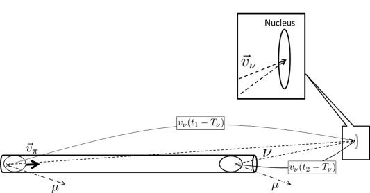
Fig. 1: The geometry of the neutrino interference experiment. The neutrino is observed by the detector at $T_{\nu}$ and produced at $t_{1}$ or $t_{2}$ in the inside of the traveling pion wave.

We investigate the physical phenomena that have a deep connection with the neutrino’s coherence and interferences in the high-energy pion decay. For simplicity we study the parameter region where the absolute value of the neutrino mass is much larger than the mass differences and the effect of the flavour oscillation is negligible. More general situations will be studied later. Other interference phenomena caused by solar neutrinos, reactor neutrinos, and others are studied in a next work.

This paper is organized in the following manner. In section 2, the sizes and shapes of wave packets are studied. In section 3, we study neutrino production amplitude in the pion decay and in section 4, we study neutrinos detection probability. The probability is expressed as the sum of normal term and new term. The position-dependent probability is obtained from the light-cone singularity of the decay correlation function in section 5. Summary and prospects are given in section 6.

2 Wave packets

In the decay of the pion Eq. $(\ref{pion-decay})$, the pion is in the beam and the neutrino is detected by the detector. Pions are produced in collisions of protons with nucleus and are superpositions of plane waves. Weak decay of a pion is studied normally using momentum eigenstates of the pion, neutrino, and muon. In the present paper, position dependent probability for the neutrino is studied and the neutrino is expressed by a wave packet, which is extended around its centers in position and momentum. In order to clarify this probability, initial pion is also expressed by a wave packet. The wave packet size is determined by the detection process for the neutrino but by the production process and medium effect for the pion.

A particle in matter is described by a wave that maintains coherence in a finite region defined by the mean free path [11]. When the particle of the finite mean free path is emitted into vacuum, the wave representing this particle propagates. This wave is expressed by a wave packet. Hence a quantum mechanical transition of this particle state is computed from the overlap integral of the wave functions. The wave function of the finite spatial size has also a finite momentum width.

We estimate the wave packet size of a proton first and those of a pion and neutrino next, following the method of our previous works [10, 11].

2.1 Size of pion wave packet

Since pions are produced in collisions of protons with nucleus, the coherence lengths of pions are determined by those of a proton and nucleus. A proton in matter interacts with nucleus and has a finite mean free path or a finite coherence length. The target nucleus has a microscopic size of order $10^{-15}$ [m] and its position is extended in a size of nucleus wave function in matter. Its magnitude is slightly larger than a nucleus intrinsic size. We use in the present paper the size of the order of $10^{-15}$ [m] for the nucleus size.

2.1.1 Proton mean free path

The mean free path of a charged particle is determined by its scattering with atoms in matter by Coulomb interaction. An energy loss is also determined by the same cross section. Data on the energy loss are summarized well in particle data summary [7] and are made use of for the evaluation of the mean free path of the proton.

The proton’s energy loss rate at the momentum, $1$ [GeV/c], for several metals such as Pb, Fe, and others are

$$-{dE\over dx}=1-2~{}[\text{MeVg}^{-1}\text{cm}^{2}],$$ (4)

hence we have the mean free path of the $1\,[\text{GeV}/c]$ proton in the material of the density $\rho$,

$$L_{\text{proton}}={E\over{dE\over dx}\times\rho}={1~{}[\text{GeV}]\over(1-2)\times 10~{}[\text{MeV g}^{-1}\text{cm}^{2}\text{g cm}^{-3}]}=50-100~{}[\text{cm}].$$ (5)

At a lower energy, $0.2\,[\text{GeV}/c]$, the energy loss rate of the proton is about $10\,[\text{MeVg}^{-1}\text{cm}^{2}]$ and the mean free path is

$$L_{\text{proton}}=10\,[\text{cm}].$$ (6)

The proton maintains coherence within the mean free path. Hence we use the mean free path for the coherence length of the proton ${\delta x}_{\text{proton}}$,

$${\delta x}_{\text{proton}}=L_{\text{proton}}.$$ (7)

When the proton of the finite coherence length is emitted into the vacuum or a system composed of dilute gas from the matter, it has the coherence length defined in matter. The proton has a constant coherence length in vacuum or in dilute gas when it is moving freely. The coherence varies when the proton is accelerated. If the potential energy $\mathcal{V}$ is added to the particle of momentum $p_{\text{before}}$, then the momentum becomes $p_{\text{after}}$ and satisfies

$$\sqrt{p_{\text{before}}^{2}+m^{2}}+\mathcal{V}=\sqrt{p_{\text{after}}^{2}+m^{2}}.$$ (8)

From Eq. $(\ref{potential-energy})$ the variants of the momentum satisfy

$$v_{\text{efore}}\times\delta p_{\text{before}}=v_{\text{after}}\times\delta p_{\text{after}},$$

$$v_{\text{before}}=\frac{p_{\text{before}}}{\sqrt{p_{\text{before}}^{2}+m^{2}}},~{}v_{\text{after}}=\frac{p_{\text{after}}}{\sqrt{p_{\text{after}}^{2}+m^{2}}}.$$ (9)

Hence the coherence length of a particle, ${\delta x}_{\text{before}}$, which is proportional to the inverse of ${\delta p}_{\text{before}}$, becomes to ${\delta x}_{\text{after}}$ after the acceleration from a velocity $v_{\text{before }}$ to a velocity $v_{\text{after}}$. The coherence length is determined by the velocity ratio,

$${\delta x}_{\text{after}}={\delta x}_{\text{before}}\times{v_{\text{after}}\over v_{\text{before}}}.$$ (10)

The velocity is bounded by the light velocity $c$, and the velocity ratio from $1\,[\text{GeV}/c]$ to $10\,[\text{GeV}/c]$ is about $1.2$ and that from $0.2\,[\text{GeV}/c]$ to $10\,[\text{GeV}/c]$ is about $5$. Hence the proton of $10~{}[\text{GeV}/c]$ regardless of the energy in matter has the mean free path

$${\delta x}_{\text{proton}}\approx 40-100~{}[\text{cm}],$$ (11)

in vacuum or a dilute gas.

2.1.2 Pion mean free path

Coherence length of pions which are produced by a proton collision with target nucleus is determined by the proton’s initial coherence length Eq.$(\ref{mfp-proton-2})$ and the target size $10^{-15}$ [m], which is negligibly small. Since the time interval of the proton wave is the same as that of the pion wave, the coherence length of the pion, ${\delta x}_{\text{pion}}$, is given from that of the proton, ${\delta x}_{\text{proton}}$, in the form

$$\frac{{\delta x}_{\text{proton}}}{v_{\text{proton}}}=\frac{{\delta x}_{\text{pion}}}{v_{\text{pion}}},~{}{\delta x}_{\text{pion}}=\frac{v_{\text{pion}}}{v_{\text{proton}}}{\delta x}_{\text{proton}}\approx{\delta x}_{\text{proton}}.$$ (12)

In relativistic energy region, particles have light velocity. Consequently from Eq. $(\ref{mfp-proton-2})$, we have the pion’s coherence of $1\,[\text{GeV}/c]$ or larger momentum

$${\delta x}_{\text{pion}}\approx 40-100~{}[\text{cm}].$$ (13)

We use this value of Eq. $(\ref{mfp-pion})$ as the size of the wave packet

$$\sqrt{\sigma_{\pi}}={\delta x}_{\text{pion}},$$ (14)

in latter sections.

In vacuum and dilute gas, pions propagate freely with the same coherence lengths. From Eqs. $(\ref{mfp-proton-1})$, $(\ref{mfp-proton-2})$, $(\ref{mfp-pion})$, the proton and pion have the coherence lengths of the order $50-100$ [cm].

2.2 Size of neutrino wave packet

A size of wave packet for observed neutrino is determined from its detection process. Neutrinos interact with nucleus or electrons in atoms incoherently and the neutrino event is identified by the reaction process in detector. Hence the size of the observed neutrino is not determined by the mean free path but by a size of the minimum physical system that the neutrino interacts and gives the signal. They are either nucleus or electrons in atom. The nucleus have sizes of order $10^{-15}$ [m] and the electron’s wave functions have sizes of order $10^{-10}$ [m]. So neutrino wave packet is either $10^{-10}$ [m] or $10^{-15}$ [m].

The interactions of the muon neutrino in detectors are

$$\nu_{\mu}+e^{-}\rightarrow e^{-}+\nu_{\mu},$$ (15)

$$\nu_{\mu}+e^{-}\rightarrow\mu^{-}+\nu_{e},$$ (16)

$$\nu_{\mu}+A\rightarrow\mu^{-}+(A+1)+X,$$ (17)

$$\nu_{\mu}+A\rightarrow\nu_{\mu}+A+X,$$ (18)

hence the size of the neutrino wave packet $\sqrt{\sigma_{\nu}}$ in processes $(\ref{numu-leptonic})$ and $(\ref{numu-lcharged})$ is of order $10^{-10}$,[m]

$$\sqrt{\sigma_{\nu}}=10^{-10}~{}[\text{m}],$$ (19)

and the neutrino wave packet $\sqrt{\sigma_{\nu}}$ in processes $(\ref{numu-hcharged})$ and $(\ref{numu-hneutral})$ is of order $10^{-15}$ [m]

$$\sqrt{\sigma_{\nu}}=10^{-15}~{}[\text{m}].$$ (20)

The interactions of the electron neutrinos in detectors are

$$\nu_{e}+e^{-}\rightarrow e^{-}+\nu_{e},$$ (21)

$$\nu_{e}+A\rightarrow e^{-}+(A+1)+X,$$ (22)

$$\nu_{e}+A\rightarrow e+A+X.$$ (23)

The neutrino wave packet $\sqrt{\sigma_{\nu}}$ in processes $(\ref{nue-leptonic})$ is of order $10^{-10}$ [m], Eq. $(\ref{mfp-neutrino-e})$, and the neutrino wave packet $\sqrt{\sigma_{\nu}}$ in processes $(\ref{nue-hcharged})$ and $(\ref{nue-hneutral})$ is of order $10^{-15}$ [m], Eq. $(\ref{mfp-neutrino-N})$. They are treated in the same way as the neutrino from the pion decay.

From Eqs. $(\ref{mfp-neutrino-e})$ and $(\ref{mfp-neutrino-N})$, the neutrino have the wave packet sizes of the order $10^{-10}$ [m] or $10^{-15}$ [m].

We study neutrinos described by the wave packets of these sizes in many particle processes. In this respect, the neutrino wave packet of the present work is different from some previous works of wave packets that are connected with flavour neutrino oscillations [17, 18, 19, 20, 21, 22, 23], where one particle properties of neutrino at production are studied. It is important to study the neutrino wave packet for our purpose of studying the interference.

2.3 Wave packet shape

A particle of the finite coherence length is described by a wave packet, which is extended in the momentum and position around the centers $({\vec{p}},{\vec{X}})$. Although its precise shape is unknown generally in real experiments, the physical quantity should have universal value that is independent from the details of wave packet. We shall obtain the physical quantity that has universal properties. The quantity that depends on the wave packet shape is neither genuine nor universal and is not important.

We give a summary of the wave packets in the following, since the wave packet may be unfamiliar to some readers. First, the wave packets are localized in the momentum and position around their centers [13, 14, 15, 16]. The whole set of the wave packets becomes complete set [10],

$$\sum_{{\vec{p}},{\vec{X}}}|{\vec{p}},{\vec{X}},\beta\rangle\langle{\vec{p}},{\vec{X}},\beta|=1,$$ (24)

independent from the shape parameter $\beta$ which is discussed later.

Second, the wave packet preserves the discrete symmetries such as invariances under space and time inversions, which have not been studied before but are quite natural, since the origin of the wave packet is the interactions of the particle with matters in detectors and the wave packet sizes are estimated in the next section under this consideration. This interaction has an origin in quantum electrodynamics that preserves parity and time reversal symmetries. So the wave packets should preserve parity and time reversal invariances. We study, hence, the wave packets which are superpositions of the plane waves around the central momentum with a weight function that has the same property under these transformations,

$$\int d\vec{k}\,w({\vec{k}};{\vec{p}}\,)e^{i(Et-{\vec{k}}\cdot{\vec{x}})},$$ (25)

where the momentum ${\vec{p}}$ is the central value of the momentum. In the present work, ${\vec{k}}$ is used for the integration variable and ${\vec{p}}$ is used for the central value of momentum.

Since the time reversal invariance is satisfied in the quantum electrodynamics and weak interactions in the lowest order, the wave packet which is invariant under the time inversion is most important. Under the time inversion, the coordinate and momentum variables are transformed into

$${\vec{x}}\rightarrow{\vec{x}},$$

$${\vec{k}}\rightarrow-{\vec{k}},\,{\vec{p}}\rightarrow-{\vec{p}}$$

$$t\rightarrow-t,$$ (26)

and the plane wave is transformed to its complex conjugate,

$$e^{i(Et-{\vec{k}}\cdot{\vec{x}})}\rightarrow e^{-i(Et-{\vec{k}}\cdot{\vec{x}})}=({e^{i(Et-{\vec{k}}\cdot{\vec{x}})}})^{*}.$$ (27)

So when the weight satisfies

$$w({\vec{k}};{\vec{p}}\,)\rightarrow(w(-{\vec{k}};-{\vec{p}}\,))=(w({\vec{k}};{\vec{p}}\,))^{*},$$ (28)

the state described by the wave packet is the superposition of the waves which are transformed equivalently under the time inversion,

$$\int d{\vec{k}}\,w({\vec{k}};{\vec{p}}\,)e^{i(Et-{\vec{k}}\cdot{\vec{x}})} \rightarrow\int d{\vec{k}}\,w(-{\vec{k}};-{\vec{p}}\,)(e^{i(Et-{\vec{k}}\cdot{\vec{x}})})^{*}$$

$$=\left(\int d{\vec{k}}\,w({\vec{k}};{\vec{p}}\,)e^{i(Et-{\vec{k}}\cdot{\vec{x}})}\right)^{*}.$$ (29)

Next we study the space inversion. Although neutrino violates this symmetry, the wave packet may preserve. Under the space inversion, the coordinate and momentum variables are changed into

$${\vec{x}}\rightarrow-{\vec{x}},\ {\vec{k}}\rightarrow-{\vec{k}},\ {\vec{p}}\rightarrow-{\vec{p}},$$ (30)

and the plane wave is changed into

$$e^{i(Et-{\vec{k}}\cdot{\vec{x}})}\rightarrow e^{i(Et-{\vec{k}}\cdot{\vec{x}})}.$$ (31)

So when the weight satisfies

$$w({\vec{k}};{\vec{p}}\,)\rightarrow w(-{\vec{k}};-{\vec{p}}\,)=w({\vec{k}};{\vec{p}}\,),$$ (32)

the state described by the wave packet is transformed in the following way,

$$\int d{\vec{k}}\,w({\vec{k}};{\vec{p}})e^{i(Et-{\vec{k}}\cdot{\vec{x}})} \rightarrow\int d{\vec{k}}\,w(-{\vec{k}};-{\vec{p}})e^{i(Et-{\vec{k}}\cdot{\vec{x}})}$$

$$~{}=\int d{\vec{k}}\,w({\vec{k}};{\vec{p}})e^{i(Et-{\vec{k}}\cdot{\vec{x}})},$$ (33)

in the same way as the plane wave.

The invariance under the time reversal, Eq. $(\ref{time-reversal})$, is a strong condition and leads the important result. We study wave packets that satisfy Eq. $(\ref{time-reversal})$. The simplest form of satisfying this property is the Gaussian wave packet $|{\vec{p}},{\vec{X}},\beta_{0}\rangle$

$$|{\vec{p}},{\vec{X}},\beta_{0}\rangle=\frac{N}{(2\pi)^{\frac{3}{2}}}\int d{\vec{k}}\,e^{-{\sigma\over 2}({\vec{k}}-{\vec{p}}\,)^{2}}e^{i\left(E({\vec{k}})(t-T)-{\vec{k}}\cdot({\vec{x}}-{\vec{X}})\right)},$$ (34)

where the parameter $\sigma$ shows the size of the wave packet in the coordinate space and $N$ is the normalization factor. We write a wave packet of a parameter $\beta$ as $|{\vec{p}},{\vec{X}},\beta\rangle$. The Gaussian wave packet is the state at $\beta=\beta_{0}$ and non-Gaussian wave packets are the states at $\beta\neq\beta_{0}$. The calculations using the Gaussian wave packet are presented in most places hereafter for the sake of simplicity, except the derivation of the large distance behavior of the neutrino wave function. It has the universal form regardless of the details of the wave packets, as far as the invariance under the time inversion holds. The theorem for the general wave packets that are invariant under the time inversion Eq. $(\ref{time-reversal})$ holds and is given in Section 4. It is worthwhile to verify the results using explicit calculations of the Gaussian wave packet or various non-Gaussian wave packets, which are made partly in the text and in the appendix.

The normal physical quantity of microscopic physics is obtained from ordinary scattering which has no dependence upon the distance or time interval between the initial and final states. This is because the length of the microscopic system is so small that the size of experimental apparatus is regarded infinite and the boundary conditions of ordinary scatterings which are defined at $t=\pm\infty$ of plane waves are suitable. Hence the amplitude and probability are defined using plane waves and the boundary conditions at $t=\pm\infty$ ensure the independence of the probability from the distance and particle’s coherence length.

For the neutrino the situation is different because the neutrino mass is so small that a new energy scale defined by ${m_{\nu}^{2}/E_{\nu}}$ becomes extremely small and a spatial length which is inversely proportional to this energy becomes macroscopic length. It is important to find a physical quantity that depends on this length, since it may give a new important information. To find a scattering amplitude and probability that have a dependence on the length or time interval, we use the amplitude defined from wave packets of finite spatial sizes, $\sigma$. Those wave packets that have central positions and are localized well around the central positions and that have the same properties in the momentum variable are suitable for this purpose. The simplest wave packets of having these properties are Gaussian wave packets Eq. $(\ref{Gaussian-wp})$ which satisfy the minimum uncertainty relation between the variances of the position and momentum. Non-Gaussian wave packet parameterized by a parameter $\beta$ and has larger uncertainties is easily defined by multiplying Hermitian polynomials to the Gaussian function.

From Eq. $(\ref{complete-set})$, the total transition probability is independent from the parameter $\beta$

$$\sum_{{\vec{p}}_{\nu},{{\vec{X}}_{\nu}}}|\langle neutrino;{\vec{p}}_{\nu},{\vec{X}}_{\nu},\beta;muon|T|pion;{\vec{p}}_{\pi},{\vec{X}}_{\pi},T_{\pi}\rangle|^{2}$$

$$=\sum_{{\vec{p}}_{\nu},{{\vec{X}}_{\nu}}}|\langle neutrino;{\vec{p}}_{\nu},{\vec{X}}_{\nu},\beta_{0};muon|T|pion;{\vec{p}}_{\pi},{\vec{X}}_{\pi},T_{\pi}\rangle|^{2},$$ (35)

which also agree to that of the plane waves. The probability of the finite distance is defined by restricting the center positions ${\vec{X}}$ in the inside of a finite spatial region $V$. The completeness condition for the function in this region $V$ is then

$$\sum_{{\vec{p}},{\vec{X}}<V}|{\vec{p}},{\vec{X}},\beta_{0}\rangle\langle{\vec{p}},{\vec{X}},\beta_{0}|=\sum_{{\vec{p}},{\vec{X}}<V}|{\vec{p}},{\vec{X}},\beta\rangle\langle{\vec{p}},{\vec{X}},\beta|,$$ (36)

and the probability satisfies

$$\sum_{{\vec{p}}_{\nu},{{\vec{X}}_{\nu}<V}}|\langle neutrino;{\vec{p}}_{\nu},{\vec{X}}_{\nu},\beta;muon|T|pion;{\vec{p}}_{\pi},{\vec{X}}_{\pi},T_{\pi}\rangle|^{2}$$

$$=\sum_{{\vec{p}}_{\nu},{{\vec{X}}_{\nu}<V}}|\langle neutrino;{\vec{p}}_{\nu},{\vec{X}}_{\nu},\beta_{0};muon|T|pion;{\vec{p}}_{\pi},{\vec{X}}_{\pi},T_{\pi}\rangle|^{2},$$ (37)

and is also independent from the $\beta$. We study the probability that is the average over a finite neutrino energy region $V_{p}$

$$\sum_{{{\vec{p}}_{\nu}<V_{p}},{{\vec{X}}_{\nu}<V}}|\langle neutrino;{\vec{p}}_{\nu},{\vec{X}}_{\nu},\beta;muon|T|pion;{\vec{p}}_{\pi},{\vec{X}}_{\pi},T_{\pi}\rangle|^{2},$$ (38)

and extract the physical quantity. For the genuine physical quantity, the value should be determined uniquely. The energy uncertainty of the neutrino experiment is of the order 10 percent of the total neutrino energy. This magnitude is the same order as that of the minimum uncertainty if the neutrino energy is $1$ [GeV]. So the minimum wave packet is applied directly in this case. The probability for a larger energy uncertainty is computed using the probability of the small energy uncertainty. The dependence of the neutrino probability on the distance will be shown to have the universal behavior.

3 Position-dependent amplitude of neutrino

Using the wave packet representation obtained in the previous section, we find the position-dependent neutrino amplitude.

3.1 Semileptonic decay of the pion

3.1.1 Weak interaction

Semileptonic decay of a pion is described by the weak Hamiltonian

$$H_{w}=g\int d{\vec{x}}\,{\partial_{\mu}}\varphi(x)J_{V-A}^{\mu}(x)=-igm_{\mu}\int d{\vec{x}}\,\varphi(x)J_{5}(x),$$

$$J_{V-A}^{\mu}(x)=\bar{\mu}(x)\gamma^{\mu}(1-\gamma_{5})\nu(x),J_{5}(x)=\bar{\mu}(x)(1-\gamma_{5})\nu(x),$$ (39)

where ${\varphi(x)}$, $\mu(x)$, and $\nu(x)$ are the pion field, muon field, and neutrino field [24]. In the above equations, $g$ is the coupling strength, $J_{V-A}^{\mu}(x)$, and $J_{5}(x)$ are the leptonic charged vector current, and leptonic pseudoscalar. The coupling is expressed with Fermi coupling $G_{F}$ and pion decay constant $f_{\pi}$,

$$g={G_{F}\over\sqrt{2}}f_{\pi}.$$ (40)

3.1.2 Neutrino production amplitude in the pion decay

When the number of the neutrino events is large enough, the distributions of the neutrino events are computed with the quantum mechanical wave functions. For the electron bi-prism experiments of Tonomura et al [25], the electrons’ interferences of the sharp energy become visible when the total number becomes significant. Even though the initial electrons have no correlation and each event occurs randomly, when number of the electrons becomes large, the signal exceeds the statistical fluctuation and the distribution shows the interference behavior. A large number of events is also necessary for the quantum mechanical interferences become visible for the neutrinos from the pion decays. In this situation each pion decay occurs randomly and its distribution is computed using quantum mechanical wave functions. We study this situation hereafter and compute the amplitude and probability quantum mechanically.

A wave function which describes a pion and its decay products satisfies a Schrödinger equation

$$i\hbar{\partial\over\partial t}|\Psi(t)\rangle=(H_{0}+H_{w})|\Psi(t)\rangle,$$ (41)

where $H_{0}$ stands for the free Hamiltonian and $H_{w}$ stands for the interaction Hamiltonian Eq. (3.1.1). The solution is

$$|\Psi(t)\rangle=|\text{pion}(t)\rangle+|\text{muon,~{}neutrino}(t)\rangle,$$

$$|\text{muon,~{}neutrino}(t)\rangle=\int_{t_{0}}^{t}{dt^{\prime}\over i\hbar}H_{w}(t^{\prime})|\text{pion}(t^{\prime})\rangle,$$ (42)

in the first order of $H_{w}$. A muon and a neutrino are described by one wave function of Eq. $(\ref{state-vector})$, $|\text{muon,~{}neutrino}(t)\rangle$, and all the informations of this system are computed from this wave function. Physical quantities were studied with this wave function [23] and the finite time interval effect was found.

Here the matrix elements between $|\text{muon,~{}neutrino}(t)\rangle$ and the state $|\mu,\nu\rangle$ defined next is studied instead of the wave function itself. Since all the informations of the wave function $|\text{muon,~{}neutrino}(t)\rangle$ are included in this matrix element, as far as a complete set of $|\mu,\nu\rangle$ is used, this matrix element is equivalent to the wave function. Furthermore the position-dependent informations on the decay process are found by the use of the wave packets. The coherent phenomenon of the neutrino which depends on the position and the neutrino detection probability are studied here with this matrix element.

The transition amplitude from a pion located around the position ${\vec{X}}_{\pi}$ to a neutrino at the position ${\vec{X}}_{\nu}$ and the muon is studied hereafter. Because the muon is not observed and all the states are summed over, the most convenient wave is used for the muon. This amplitude is

$$T=\int d^{4}x\,\langle{\mu},{\nu}|H_{w}(x)|\pi\rangle,$$ (43)

where the states are described by the wave packets of central values of momenta and coordinates and the widths in the form

$$|\pi\rangle=|{\vec{p}}_{\pi},{\vec{X}}_{\pi},T_{\pi}\rangle,\ |\mu,\nu\rangle=|\mu,{\vec{p}}_{\mu};\nu,{\vec{p}}_{\nu},{\vec{X}}_{\nu},T_{\nu}\rangle.$$ (44)

The states are defined by the matrix elements,

$$\langle 0|\varphi(x)|{\vec{p}}_{\pi},{\vec{X}}_{\pi},T_{\pi}\rangle=N_{\pi}\rho_{\pi}\int d{\vec{k}_{\pi}}\,e^{-{\sigma_{\pi}\over 2}({\vec{k}}_{\pi}-{\vec{p}}_{\pi})^{2}}e^{-i\left(E({\vec{k}}_{\pi})(t-T_{\pi})-i{\vec{k}}_{\pi}\cdot({\vec{x}}-{\vec{X}}_{\pi})\right)}$$

$$\approx N_{\pi}\rho_{\pi}\left({2\pi\over\sigma_{\pi}}\right)^{\frac{3}{2}}e^{-{1\over 2\sigma_{\pi}}\left({\vec{x}}-{\vec{X}_{\pi}}-{\vec{v}}_{\pi}(t-T_{\pi})\right)^{2}}e^{-i\left(E({\vec{p}}_{\pi})(t-T_{\pi})-i{\vec{p}}_{\pi}\cdot({\vec{x}}-{\vec{X}}_{\pi})\right)},$$ (45)

$$\langle\mu,{\vec{p}}_{\mu};\nu,{\vec{p}}_{\nu},{\vec{X}}_{\nu},T_{\nu}|\bar{\mu}(x)(1-\gamma_{5})\nu(x)|0\rangle$$

$$=\frac{N_{\nu}}{(2\pi)^{{3}}}\int d{\vec{k}}_{\nu}e^{-{\sigma_{\nu}\over 2}({\vec{k}}_{\nu}-{\vec{p}}_{\nu})^{2}}\left({m_{\mu}\over E({\vec{p}}_{\mu})}\right)^{\frac{1}{2}}\left({m_{\nu}\over E({\vec{k}}_{\nu})}\right)^{\frac{1}{2}}\bar{u}({\vec{p}}_{\mu})(1-\gamma_{5})\nu({\vec{k}}_{\nu})$$

$$\times e^{i\left(E({\vec{p}}_{\mu})t-{\vec{p}}_{\mu}\cdot{\vec{x}}\right)}e^{i\left(E({\vec{k}}_{\nu})(t-T_{\nu})-{\vec{k}}_{\nu}\cdot({\vec{x}}-{\vec{X}}_{\nu})\right)},$$ (46)

where

$$N_{\pi}=\left(\frac{\sigma_{\pi}}{\pi}\right)^{\frac{3}{4}},~{}N_{\nu}=\left(\frac{\sigma_{\nu}}{\pi}\right)^{\frac{3}{4}},\rho_{\pi}=\left(\frac{1}{2E_{\pi}(2\pi)^{3}}\right)^{\frac{1}{2}}.$$ (47)

In this paper the spinor’s normalization is

$$\sum_{s}u(p,s)\bar{u}(p,s)={\gamma\cdot p+m\over 2m}.$$ (48)

In the above equation the pion’s life time is ignored. The sizes, $\sigma_{\pi}$ and $\sigma_{\nu}$, in Eqs. $(\ref{pion-wf})$ and $(\ref{mu-nu-wf})$ are sizes of the pion wave packet and of the neutrino wave packet. Minimum wave packets are used in most of the present paper but non-minimum wave packets are studied and it is shown that our results are the same.

From the results of the previous section, the size of pion wave packet is of the order $0.5-1.0$ [m] and the momentum has a small width. So the pion momentum is integrated easily, and is replaced with its central value ${\vec{p}}_{\pi}$ and the final expression of Eq. $(\ref{pion-wf})$ is obtained. For the neutrino, the size of wave packet should be the size of minimum physical system that a neutrino interacts, i.e., the nucleus. Hence to study neutrino interferences, we use the nuclear size for $\sigma_{\nu}$.

The amplitude $T$ for one pion to decay into a neutrino and a muon is written in the form

$$T=\int dtd{\vec{x}}T(t,{\vec{x}}),T(t,{\vec{x}})=\int d{\vec{k}}_{\nu}T(t,{\vec{x}},k_{\nu})$$ (49)

where

$$T(t,{\vec{x}},k_{\nu}) = igm_{\mu}N^{\prime\prime}e^{-{1\over 2\sigma_{\pi}}\left({\vec{x}}-{\vec{X}_{\pi}}-{\vec{v}}_{\pi}(t-T_{\pi})\right)^{2}}e^{-i\left(E({\vec{p}}_{\pi})(t-T_{\pi})-i{\vec{p}}_{\pi}\cdot({\vec{x}}-{\vec{X}}_{\pi})\right)}$$

$$\times e^{i\left(E(\vec{p}_{\mu})t-{\vec{p}}_{\mu}\cdot{\vec{x}}\right)}\bar{u}({\vec{p}}_{\mu})(1-\gamma_{5})\nu({\vec{k}}_{\nu})e^{i\left(E({\vec{k}}_{\nu})(t-T_{\nu})-{\vec{k}}_{\nu}\cdot({\vec{x}}-{\vec{X}}_{\nu})\right)-\frac{\sigma_{\nu}}{2}({\vec{k}}_{\nu}-{\vec{p}}_{\nu})^{2}},$$

$$N^{\prime\prime} = N_{\pi}N_{\nu}\left({2\pi\over\sigma_{\pi}}\right)^{\frac{3}{2}}N_{0},~{}N_{0}=\left(\frac{m_{\mu}m_{\nu}}{E_{\mu}E_{\nu}}\right)^{\frac{1}{2}}\times\frac{\rho_{\pi}}{(2\pi)^{3}}.$$ (50)

This amplitude depends upon the coordinates $(t,{\vec{x}})$ explicitly and is not invariant under the translation.

3.2 Neutrino wave function

We integrate the neutrino momentum of Eq. $(\ref{amplitude})$ by applying Gaussian integral and find the coordinate representation of the neutrino wave function. It is found that a phase of neutrino wave function has a particular form that is proportional to the square of the mass and inversely proportional to the neutrino energy.

3.2.1 Phase of neutrino wave function

For not so large $t-T_{\nu}$ region, ${\vec{k}}_{\nu}$ is integrated around the central momentum ${\vec{p}}_{\nu}$ in Eq. $(\ref{amplitude})$. The amplitude becomes,

$$T(t,{\vec{x}}) = igm_{\mu}\tilde{N}e^{-{1\over 2\sigma_{\pi}}\left({\vec{x}}-{\vec{X}_{\pi}}-{\vec{v}}_{\pi}(t-T_{\pi})\right)^{2}}e^{-i\left(E({\vec{p}}_{\pi})(t-T_{\pi})-i{\vec{p}}_{\pi}\cdot({\vec{x}}-{\vec{X}}_{\pi})\right)}e^{iE({\vec{p}}_{\mu})t-i{\vec{p}}_{\mu}\cdot{\vec{x}}}$$ (51)

$$\times\bar{u}({\vec{p}}_{\mu})(1-\gamma_{5})\nu({\vec{p}}_{\nu})e^{i\phi(x)}e^{-{1\over 2\sigma_{\nu}}({\vec{x}}-{\vec{X}}_{\nu}-{\vec{v}}_{\nu}(t-T_{\nu}))^{2}},$$

where $\tilde{N}$ is the normalization factor, ${\vec{v}}_{\nu}$ is the neutrino velocity, and $\phi$ is the phase of neutrino wave function. They are given by

$$\tilde{N}=N_{\pi}N_{\nu}\left(\frac{2\pi}{\sigma_{\pi}}\right)^{\frac{3}{2}}\left(\frac{2\pi}{\sigma_{\nu}}\right)^{\frac{3}{2}}N_{0},$$ (52)

$$\phi(x)=E({\vec{p}}_{\nu})(t-T_{\nu})-{\vec{p}}_{\nu}\!\cdot\!({\vec{x}}-{\vec{X}}_{\nu}).$$ (53)

The phase $\phi(x)$ is rewritten for a small wave packet by substituting the central value ${\vec{x}}$ of neutrino’s Gaussian function

$${\vec{x}}={\vec{X}}_{\nu}+{\vec{v}}_{\nu}(t-T_{\nu}),$$ (54)

in the form

$$\bar{\phi}_{g}(t-T_{\nu}) = E({\vec{p}}_{\nu})(t-T_{\nu})-{\vec{p}}_{\nu}\cdot{\vec{v}}_{\nu}(t-T_{\nu})$$ (55)

$$= {E^{2}_{\nu}(\vec{p}_{\nu})-{\vec{p}}_{\nu}^{~{}2}\over E_{\nu}({\vec{p}}_{\nu})}(t-T_{\nu})={m_{\nu}^{2}\over E_{\nu}(\vec{p}_{\nu})}(t-T_{\nu}),$$

which has a typical form of the relativistic particle. The phase becomes proportional to the neutrino mass squared and inversely proportional to the neutrino energy. The magnitude of the phase at the position Eq. $(\ref{center-coordinate})$ is small due to the cancellation between the oscillation in time and space. This cancellation does not occur in the derivatives of the phase with respect to the coordinate, which are given in the form

$$\frac{\partial}{\partial x_{\mu}}\phi=p_{\nu}^{\mu}.$$ (56)

This is not proportional to the square of neutrino mass but is determined by the energy and momentum.

When the position is moving with the light velocity

$${\vec{x}}={\vec{X}}_{\nu}+{\vec{c}}(t-T_{\nu}),\ |{\vec{c}}\,|=1,$$ (57)

then the phase is given by

$$\bar{\phi}_{c}(t-T_{\nu})=E({\vec{p}}_{\nu})(t-T_{\nu})-{\vec{p}}_{\nu}\!\cdot{\vec{c}}\,(t-T_{\nu})=\frac{m_{\nu}^{2}}{2E_{\nu}(\vec{p}_{\nu})}(t-T_{\nu}),$$ (58)

and becomes a half of $\bar{\phi_{g}}$.

Interference of the neutrino due to this slow phase of the energy $E_{\nu}$ and $E_{\nu}+\Delta E_{\nu}$ is identical if the neutrino phase $\bar{\phi}_{c}$ satisfies

$$\Delta\bar{\phi}_{c}=\delta E_{\nu}{\partial\over\partial E_{\nu}}\bar{\phi}_{c}\ll\pi.$$ (59)

Hence the neutrinos of the energy width $\Delta E_{\nu}$ show the same interference. We will see later that this is actually satisfied for the light neutrino of the energy width around $100$ [MeV].

The slow phase $\bar{\phi_{c}}$ of Eq. $(\ref{light-phase})$ is a characteristic feature of the neutrino, and is the intrinsic property of the neutrino wave function along the light cone. Using the Gaussian wave packet, this phase has been obtained easily. Since this phase is genuine of the neutrino wave function, the same behavior is obtained in more general cases including the spreading wave packet or non-Gaussian wave packets. The spreading of the wave packet is negligible in the longitudinal direction and is not so small in the transverse direction. Its effect has been ignored for simplicity in this section and will be studied in the latter section and appendix. It will be shown there that the spreading of the wave packet in the transverse direction modifies the ${\vec{k}}_{\nu}$ integration but the final result turns actually into the same. For general wave packets, if the completeness, Eq. $(\ref{completeness-finite-volume})$ is applied, the total probability satisfies Eq. $(\ref{completeness-finite-volume2})$. The transition amplitude in this case has the same phase $\phi(x)$, Eq. $(\ref{neutrino-phase})$ and is written in the form,

$$T(t,{\vec{x}}) = igm_{\mu}\tilde{N}e^{-{1\over 2\sigma_{\pi}}\left({\vec{x}}-{\vec{X}_{\pi}}-{\vec{v}}_{\pi}(t-T_{\pi})\right)^{2}}e^{-i\left(E({\vec{p}}_{\pi})(t-T_{\pi})-i{\vec{p}}_{\pi}\cdot({\vec{x}}-{\vec{X}}_{\pi})\right)}e^{i(E({\vec{p}}_{\mu})t-{\vec{p}}_{\mu}\cdot{\vec{x}})}$$ (60)

$$\times \bar{u}({\vec{p}}_{\mu})(1-\gamma_{5})\nu({\vec{p}}_{\nu})e^{i\phi(x)}w\left({\vec{x}}-{\vec{X}}_{\nu}-{\vec{v}}_{\nu}(t-T_{\nu})\right),$$

where $w({\vec{x}})$ is the amplitude of neutrino wave function obtained by the Fourier transformation from the $w({\vec{p}},{\vec{k}})$. The spreading effect is negligible for the small time interval and $w({\vec{x}})$ is given in the form

$$w({\vec{x}})=\int d\tilde{\vec{k}}e^{i\tilde{\vec{k}}\cdot{\vec{x}}}w({\tilde{\vec{k}}}),~{}\tilde{\vec{k}}={\vec{k}}-{\vec{p}},$$ (61)

and decreases fast with $|{\vec{x}}|$. Moreover from Eq. $(\ref{time-reversal})$, this function is real function

$$w({\vec{x}})=w({\vec{x}})^{*},$$ (62)

which leads the universal long-distance behavior to the neutrino probability. The spreading effect is included when the long-range component of the correlation is studied in Section 4.

3.2.2 Position-dependence, energy momentum non-conservation, and interferences

When the space-time coordinates $(t,{\vec{x}})$ are integrated in the amplitude of the plane waves, the delta function of the energy and momentum conservation emerges. The scattering amplitude with this delta function shows that the final states have the same energy and momentum with the initial state. On the other hand, the position-dependent amplitude $T$ for the wave packets is not invariant under the translation and has no delta function. So the energy and momentum of the final state are not necessary the same as the initial state. The states which do not satisfy the energy and momentum conservation should be included to get consistent results from the completeness. This amplitude shows the position-dependent behavior, from which a new information is found.

Let us compare the neutrino velocity with the light velocity. The neutrino of energy $1~{}[\text{GeV}]$ and the mass $1~{}[\text{eV}/c^{2}]$ has a velocity

$$v/c=1-2\epsilon,\ \epsilon=\left({m_{\nu}c^{2}\over E_{\nu}}\right)^{2}=5\times 10^{-19},$$ (63)

hence the neutrino propagates the distance $l$, where

$$l=l_{0}(1-\epsilon)=l_{0}-\delta l,\delta l=l_{0}\times\epsilon,$$ (64)

while the light propagates the distance $l_{0}$. This difference of distance, $\delta l$, becomes

$$\delta l=5\times 10^{-17}~{}[\text{m}];~{}l_{0}=100~{}[\text{m}],$$ (65)

$$\delta l=5\times 10^{-16}~{}[\text{m}];~{}l_{0}=1000~{}[\text{m}],$$ (66)

which are much smaller than the sizes of the above wave packets Eq. $(\ref{mfp-pion})$. This gives the important effect for the neutrino amplitude at the nuclear target or the atom target to show interference. The geometry of the neutrino interference is shown in Fig. 1. The neutrino wave produced at a time $t_{1}$ arrives to one nucleus or atom in the detector and is added to the wave produced at $t_{2}$ and arrives to the same nucleus or atom same time. A constructive interference of waves is shown in the text.

4 Position-dependent probability and interference

The probability of detecting neutrino at a finite distance is studied in this section. Particularly the finite-time interval T correction, i.e., the deviation of the transition probability from the T-linear form, is obtained. For this purpose, the total probability is expressed with the two point correlation function of decay process, which has the light-cone singularity. The light-cone singularity leads the finite-distance correction of universal form.

4.1 Transition probability

The transition probability of a pion of momentum ${\vec{p}}_{\pi}$ located at space-time position $(T_{\pi},{\vec{X}}_{\pi})$ to a neutrino of momentum ${\vec{p}}_{\nu}$ at space-time position $(T_{\nu},{\vec{X}}_{\nu})$ and a muon of momentum ${\vec{p}}_{\mu}$ is written in the form

$$|T|^{2} = g^{2}m_{\mu}^{2}|\tilde{N}|^{2}\int d^{4}x_{1}d^{4}x_{2}S_{5}(s_{1},s_{2})$$ (67)

$$\times e^{i(\phi(x_{1})-\phi(x_{2}))}e^{-{1\over 2\sigma_{\nu}}\left({\vec{x}}_{1}-{\vec{X}}_{\nu}-{\vec{v}}_{\nu}(t_{1}-T_{\nu})\right)^{2}}e^{-{1\over 2\sigma_{\nu}}\left({\vec{x}}_{2}-{\vec{X}}_{\nu}-{\vec{v}}_{\nu}(t_{2}-T_{\nu})\right)^{2}}$$

$$\times e^{-i\left(E({\vec{p}}_{\pi})(t_{1}-T_{\pi})-{\vec{p}}_{\pi}\cdot({\vec{x}}_{1}-{\vec{X}}_{\pi})\right)}e^{i\left(E({\vec{p}}_{\pi})(t_{2}-T_{\pi})-{\vec{p}}_{\pi}\cdot({\vec{x}}_{2}-{\vec{X}}_{\pi})\right)}$$

$$\times e^{i\left(E({\vec{p}}_{\mu})t_{1}-{\vec{p}}_{\mu}\cdot{\vec{x}}_{1}\right)}e^{-i\left(E({\vec{p}}_{\mu})t_{2}-{\vec{p}}_{\mu}\cdot{\vec{x}}_{2}\right)}$$

$$\times e^{-{1\over 2\sigma_{\pi}}\left({\vec{x}}_{1}-{\vec{X}_{\pi}}-{\vec{v}}_{\pi}(t_{1}-T_{\pi})\right)^{2}}e^{-{1\over 2\sigma_{\pi}}\left({\vec{x}}_{2}-{\vec{X}_{\pi}}-{\vec{v}}_{\pi}(t_{2}-T_{\pi})\right)^{2}},$$

where $S_{5}(s_{1},s_{2})$ stands for the products of Dirac spinors and their complex conjugates,

$$S_{5}(s_{1},s_{2})=\left(\bar{u}({\vec{p}}_{\mu})(1-\gamma_{5})\nu({{\vec{p}}_{\nu}})\right)\left(\bar{u}({\vec{p}}_{\mu})(1-\gamma_{5})\nu({{\vec{p}}_{\nu}})\right)^{*},$$ (68)

and its spin summation is given by

$$S^{5} = \sum_{s_{1},s_{2}}S^{5}(s_{1},s_{2})=\frac{2}{m_{\nu}m_{\mu}}(p_{\mu}\!\cdot\!p_{\nu}).$$ (69)

For the plane waves, the coordinates $x_{1}$ and $x_{2}$ are integrated easily and $(\delta^{(4)}(p_{f}-p_{i}))^{2}=\delta^{(4)}(p_{f}-p_{i})\delta^{(4)}(0)$ is obtained. Thus the four dimensional momentum is conserved and the probability is proportional to the volume $V$, which is cancelled with the normalization factor and T from $\delta^{(4)}(0)=V\text{T}$. The probability is proportional to T and the proportional constant gives the decay rate per time. Here we calculate the finite-time interval correction for the neutrino detection process. The neutrino is observed through the interaction with the nucleus and is expressed with the wave packet. In order to obtain the finite-time interval correction, we write the probability with the correlation function of the pion and muon system. The transition probability which is integrated in momenta of the final state and average over the initial momentum is written, then, in the form

$$\int d{\vec{p}}_{\pi}\rho_{exp}({\vec{p}}_{\pi})d{\vec{p}}_{\mu}d{\vec{p}}_{\nu}\sum_{s_{1},s_{2}}|T|^{2}$$

$$=g^{2}m_{\mu}^{2}|N_{\pi\nu}|^{2}\frac{2}{(2\pi)^{3}}\int d{\vec{p}}_{\nu}\rho_{\nu}^{2}d^{4}x_{1}d^{4}x_{2}e^{-{1\over 2\sigma_{\nu}}\left({\vec{x}}_{1}-{\vec{X}}_{\nu}-{\vec{v}}_{\nu}(t_{1}-T_{\nu})\right)^{2}}e^{-{1\over 2\sigma_{\nu}}\left({\vec{x}}_{2}-{\vec{X}}_{\nu}-{\vec{v}}_{\nu}(t_{2}-T_{\nu})\right)^{2}}$$

$$\times\Delta_{\pi,\mu}(\delta t,\delta{\vec{x}})e^{i\phi(\delta x_{\mu})}e^{-{1\over 2\sigma_{\pi}}\left({\vec{x}}_{1}-{\vec{X}_{\pi}}-\bar{\vec{v}}_{\pi}(t_{1}-T_{\pi})\right)^{2}}e^{-{1\over 2\sigma_{\pi}}\left({\vec{x}}_{2}-{\vec{X}_{\pi}}-\bar{\vec{v}}_{\pi}(t_{2}-T_{\pi})\right)^{2}},$$

$$N_{\pi\nu}=\left(\frac{4\pi}{\sigma_{\pi}}\right)^{\frac{3}{4}}\left(\frac{4\pi}{\sigma_{\nu}}\right)^{\frac{3}{4}},~{}\rho_{\nu}=\left(\frac{1}{2E_{\nu}(2\pi)^{3}}\right)^{\frac{1}{2}},~{}\delta x=x_{1}-x_{2},$$ (70)

using the correlation function $\Delta_{\pi,\mu}(\delta t,\delta{\vec{x}})$. The correlation function is defined with a pion’s momentum distribution $\rho_{exp}({\vec{p}}_{\pi})$, by

$$\Delta_{\pi,\mu}(\delta t,\delta{\vec{x}})={\frac{1}{(2\pi)^{3}}}\int{d{\vec{p}}_{\pi}\over E({\vec{p}}_{\pi})}\rho_{exp}({\vec{p}}_{\pi}){d{\vec{p}}_{\mu}\over E({\vec{p}}_{\mu})}(p_{\mu}\!\cdot\!p_{\nu})e^{-i\left(\{E({\vec{p}}_{\pi})-E({\vec{p}}_{\mu})\}\delta t-({\vec{p}}_{\pi}-{\vec{p}}_{\mu})\cdot\delta{\vec{x}})\right)}.$$ (71)

In the above equation, Eqs. (55) and (56) were substituted. The muon momentum is integrated in whole positive energy region, because the muon is not observed. If the muon is observed and its momentum is measured together with the neutrino, then the muon momentum is integrated in the finite-energy region as in the inclusive hadron reactions [26]. Pion momentum is integrated in the region specified by the initial pion beam. The velocity ${\vec{v}}_{\pi}$ in the pion Gaussian factor was replaced with its average $\bar{\vec{v}}_{\pi}$. This is verified from the large spatial size of the pion wave packet discussed in the previous section. If the pion’s momentum is fixed to one value, the correlation function

$$\tilde{\Delta}_{\pi,\mu}(\delta t,\delta{\vec{x}})={\frac{1}{(2\pi)^{3}}}{1\over E({\vec{p}}_{\pi})}\int{d{\vec{p}}_{\mu}\over E({\vec{p}}_{\mu})}(p_{\mu}\!\cdot\!p_{\nu})e^{-i\left(\{E({\vec{p}}_{\pi})-E({\vec{p}}_{\mu})\}\delta t-({\vec{p}}_{\pi}-{\vec{p}}_{\mu})\cdot\delta{\vec{x}}\right)}$$ (72)

is used instead of Eq.$(\ref{pi-mucorrelation})$.

4.2 Light-cone singularity

The correlation function $\tilde{\Delta}_{\pi,\mu}(\delta t,\delta{\vec{x}})$ has a singularity near the light-cone region

$$\lambda=\delta t^{2}-{\left|\delta\vec{x}\right|}^{2}=0,$$ (73)

which is extended into a large $|\delta{\vec{x}}|$ and is independent from ${\vec{p}}_{\pi}$. So $\Delta_{\pi,\mu}(\delta t,\delta{\vec{x}})$ has the same light-cone singularity. So the probability Eq. $(\ref{probability-correlation})$ has a large finite-distance correction due to the singularity of $\Delta_{\pi,\mu}(\delta t,\delta{\vec{x}})$. We find the light-cone singularity of $\tilde{\Delta}_{\pi,\mu}(\delta t,\delta{\vec{x}})$ [27] in the following and apply the result also to $\Delta_{\pi,\mu}(\delta t,\delta{\vec{x}})$.

4.2.1 Separation of singularity

If the particles are plane waves, the energy and momentum are strictly conserved and the momenta satisfy

$$p_{\pi}=p_{\mu}+p_{\nu},\ (p_{\pi}-p_{\mu})^{2}=m_{\nu}^{2}\approx 0.$$ (74)

Hence the momentum difference $p_{\pi}-p_{\mu}$ is almost on the light cone and the $\Delta_{\pi,\mu}(\delta t,\delta{\vec{x}})$ around the light cone, $\lambda=0$, is important in Eq.$(\ref{probability-correlation})$. In order to extract the singular term from $\tilde{\Delta}_{\pi,\mu}(\delta t,\delta{\vec{x}})$, we write the integral in the form

$$\tilde{\Delta}_{\pi,\mu}(\delta t,\delta{\vec{x}})={\frac{1}{(2\pi)^{3}}}{1\over E({\vec{p}}_{\pi})}I(p_{\pi},\delta x),$$

$$I(p_{\pi},\delta x)={2\over\pi}\int d^{(4)}p_{\mu}\,\theta(p_{\mu}^{0})(p_{\mu}\!\cdot\!p_{\nu})\text{Im}\left[1\over p_{\mu}^{2}-m_{\mu}^{2}-i\epsilon\right]e^{-i\left(\{E({\vec{p}}_{\pi})-E({\vec{p}}_{\mu})\}\delta t-({\vec{p}}_{\pi}-{\vec{p}}_{\mu})\cdot\delta{\vec{x}}\right)}.$$ (75)

Next the integration variable is changed from $p_{\mu}$ to $q=p_{\mu}-p_{\pi}$ that is conjugate to $\delta x$. We have then

$$I(p_{\pi},\delta x) ={2\over\pi}\int d^{4}q\,\theta(q^{0}+p_{\pi}^{0})((p_{\pi}+q)\!\cdot\!p_{\nu})\text{Im}\left[1\over(q+p_{\pi})^{2}-m_{\mu}^{2}-i\epsilon\right]e^{iq\cdot\delta x}$$

$$=(p_{\pi}\!\cdot\!p_{\nu}){2\over\pi}\int d^{4}q\,\theta(q^{0}+p_{\pi}^{0})\text{Im}\left[1\over(q+p_{\pi})^{2}-m_{\mu}^{2}-i\epsilon\right]e^{iq\cdot\delta x}$$

$$+{2\over\pi}\int d^{4}q\,\theta(q^{0}+p_{\pi}^{0})(q\!\cdot\!p_{\nu})\text{Im}\left[1\over(q+p_{\pi})^{2}-m_{\mu}^{2}-i\epsilon\right]e^{iq\!\cdot\!\delta x},$$ (76)

and we separate the integration region into two parts:

$$I(p_{\pi},\delta x)=I_{1}(p_{\pi},\delta x)+I_{2}(p_{\pi},\delta x),$$

$$I_{1}(p_{\pi},\delta x)=\left\{p_{\pi}\!\cdot\!p_{\nu}+p_{\nu}\!\cdot\!\left(-i{\partial\over\partial\delta x}\right)\right\}\tilde{I}_{1},$$

$$\tilde{I}_{1}={2\over\pi}\int d^{4}q\,\theta(q^{0})\text{Im}\left[1\over(q+p_{\pi})^{2}-m_{\mu}^{2}-i\epsilon\right]e^{iq\cdot\delta x},$$

$$I_{2}(p_{\pi},\delta x)={2\over\pi}\int_{-p_{\pi}^{0}}^{0}dq^{0}d^{3}q\,p_{\nu}\!\cdot\!(p_{\pi}+q)\text{Im}\left[1\over(q+p_{\pi})^{2}-m_{\mu}^{2}-i\epsilon\right]e^{iq\cdot\delta x}.$$ (77)

$I_{1}(p_{\pi},\delta x)$ is the integral of the region $0\leq q^{0}$ and has a singularity and $I_{2}(p_{\pi},\delta x)$ is the integral of the region $-p_{\pi}^{0}\leq q^{0}\leq 0$ and is regular. Although the large finite-distance correction is derived from the singular term $I_{1}(p_{\pi},\delta x)$, $I_{1}$ does not contribute to the total probability at an infinite time for the plane waves. Conversely $I_{2}(p_{\pi},\delta x)$ contributes to the total probability without finite-distance correction for the plane waves. Consequently by expressing $I$ into the sum of $I_{1}$ and $I_{2}$, the correction at finite distance is found easily. So the physical quantity at the finite distance that reflects interference is computed using the most singular term of $I_{1}$.

4.2.2 Correlation function

The denominator of the integrand of $\tilde{I}_{1}$ is expanded in $p_{\pi}\!\cdot\!q$ and the $\tilde{I}_{1}$ is written in the form

$$\tilde{I}_{1}(p_{\pi},\delta x)={2\over\pi}\int d^{4}q\,\theta(q^{0})~{}\text{Im}\left[{1\over q^{2}+m_{\pi}^{2}-m_{\mu}^{2}+2q\!\cdot\!p_{\pi}-i\epsilon}\right]e^{iq\cdot\delta x}$$

$$={2\over\pi}\int d^{4}q\,\theta(q^{0})~{}\text{Im}\left[{1\over q^{2}+{\tilde{m}}^{2}-i\epsilon}-2p_{\pi}\!\cdot\!q\left({1\over q^{2}+{\tilde{m}}^{2}-i\epsilon}\right)^{2}+\cdots\right]e^{iq\cdot\delta x}$$

$$={2\over\pi}\int d^{4}q\,\theta(q^{0})\left\{1-2p_{\pi}\!\cdot\!\left(-i{\partial\over\partial\delta x}\right){\partial\over\partial{\tilde{m}}^{2}}+\cdots\right\}\,\text{Im}\left[{1\over q^{2}+{\tilde{m}}^{2}-i{\epsilon}}\right]e^{iq\cdot\delta x}$$

$$=2\left\{1-2p_{\pi}\!\cdot\!\left(-i{\partial\over\partial\delta x}\right){\partial\over\partial{\tilde{m}}^{2}}+\cdots\right\}\int d^{4}q\,\theta(q^{0})\delta(q^{2}+{\tilde{m}}^{2})e^{iq\cdot\delta x},$$ (78)

where

$${\tilde{m}}^{2}=m_{\pi}^{2}-m_{\mu}^{2}.$$ (79)

The expansion in $2q\!\cdot\!p$ of Eq. $(\ref{singular-function})$ converges in the region

$${2p_{\pi}\!\cdot\!q\over q^{2}+{\tilde{m}}^{2}}<1.$$ (80)

Here $q$ is the integration variable and varies. So we evaluate the series after the integral and find the condition for the convergence. We find later that the series after the momentum integration converges in the region

$${2p_{\pi}\!\cdot\!p_{\nu}\over{\tilde{m}}^{2}}\leq 1.$$ (81)

So the following result that is obtained using this expansion is applied in this kinematical region. In the outside of this region, the evaluation of the integrals $I_{1}$ and $I_{2}$ separately is not useful and $I$ is integrated directly.

The formula for a relativistic field of the imaginary mass

$$\int d^{4} q\,\theta(q^{0})\delta(q^{2}+{\tilde{m}}^{2})e^{iq\cdot\delta x}=(2\pi)^{3}i\left[{1\over 4\pi}\delta(\lambda)\epsilon(\delta t)+f_{short}\right],$$

$$f_{short} =-{i{\tilde{m}}\over 8\pi\sqrt{-\lambda}}\theta(-{\lambda})\left\{N_{1}\left(\tilde{m}\sqrt{-\lambda}\right)-i\epsilon(\delta t)J_{1}\left(\tilde{m}\sqrt{-\lambda}\right)\right\}$$

$$-\theta(\lambda){i\tilde{m}\over 4\pi^{2}\sqrt{\lambda}}K_{1}\left(\tilde{m}\sqrt{\lambda}\right),$$ (82)

where $N_{1}$, $J_{1}$, and $K_{1}$ are Bessel functions, is substituted to Eq. $(\ref{singular-function})$.

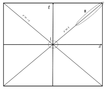
Fig. 2: The region I corresponds to short-range correlation where $t\sim x\sim 0$. On the other hand the region II corresponds to long-range correlation where $t^{2}-x^{2}\sim 0$ and both $t$ and $x$ can be macroscopic.

The first term in the right hand side of Eq. $(\ref{singular-function-f})$ is the most singular term and the second and third terms have singularity of the form $1/\lambda$ around $\lambda=0$ and decrease as $e^{-\tilde{m}\sqrt{|\lambda}|}$ or oscillates as $e^{i\tilde{m}\sqrt{|\lambda}|}$. The singular functions and regular functions behave differently and are expressed in Fig. 2 for one space dimension. The singular functions have the value around the light cone and the regular functions have finite value in small area around the origin. Since the light cone is extended in macroscopic area, the light-cone singularity leads the correlation function to become long-range. The long-range correlation function from the light-cone singularity and the short-range correlation function from the regular function are computed next. Thus the correlation function $\tilde{I}_{1}$ becomes long-range only along the light-cone region and decreases exponentially or oscillates rapidly in other directions. So $\tilde{I}_{1}(p_{\pi},\delta x)$ then is written in the form

$$\tilde{I}_{1}(p_{\pi},\delta x)=2(2\pi)^{3}i\left\{1-2p_{\pi}\!\cdot\!\left(-i{\partial\over\partial\delta x}\right){\partial\over\partial{\tilde{m}}^{2}}+\cdots\right\}\left({1\over 4\pi}\delta(\lambda)\epsilon(\delta t)+f_{short}\right).$$ (83)

Next $I_{2}$ is evaluated. For $I_{2}$ we use the momentum $\tilde{q}=q+p_{\pi}$ and to write in the form

$$I_{2}(p_{\pi},\delta x)=\frac{2}{\pi}\int_{0<\tilde{q}^{0}<p_{\pi}^{0}}d^{4}\tilde{q}\,(p_{\nu}\!\cdot\!\tilde{q})\text{Im}\left[\frac{1}{\tilde{q}^{2}-m_{\mu}^{2}-i\epsilon}\right]e^{i(\tilde{q}-p_{\pi})\cdot\delta x}$$

$$=e^{i(-p_{\pi})\cdot\delta x}\left\{p_{\nu}\!\cdot\!\left(-i{\partial\over\partial\delta x}\right)\right\}{2\over\pi}\int_{0<\tilde{q}^{0}<p_{\pi}^{0}}d^{4}\tilde{q}\,\pi\delta(q^{2}-m_{\mu}^{2})e^{i\tilde{q}\cdot\delta x}$$

$$=e^{-ip_{\pi}\cdot\delta x}\left\{p_{\nu}\!\cdot\!\left(-i{\partial\over\partial\delta x}\right)\right\}\int{d^{3}q\over\sqrt{q^{2}+m_{\mu}^{2}}}\theta\left(p_{\pi}^{0}-\sqrt{q^{2}+m_{\mu}^{2}}\right)e^{iq\cdot\delta x}.$$ (84)

The regular part $I_{2}$ has no singularity because the integration domain is finite and becomes short-range.

Thus the first term in $\tilde{I}_{1}$ gives a finite long-distance correlation and the rests, the second term in $I_{1}$ and $I_{2}$, give short distance correlations. The correlation function, $\tilde{\Delta}_{\pi,\mu}(\delta t,\delta{\vec{x}})$ has a singular term and a regular term and is written in the form

$$\tilde{\Delta}_{\pi,\mu}(\delta t,\delta{\vec{x}})={1\over(2\pi)^{3}}{1\over E(p_{\pi})}\Biggl{[}\left\{p_{\pi}\!\cdot\!p_{\nu}+p_{\nu}\!\cdot\!\left(-i\frac{\partial}{\partial\delta x}\right)\right\}2(2\pi)^{3}i$$

$$\left\{1-2p_{\pi}\!\cdot\!\left(-i{\partial\over\partial\delta x}\right){\partial\over\partial{\tilde{m}}^{2}}+\cdots\right\}\left(\frac{1}{4\pi}\delta(\lambda)\epsilon(\delta t)+f_{short}\right)+I_{2}\Biggr{]},$$ (85)

where the dots stand for the higher order terms.

4.3 Integration of spatial coordinates

Next, the coordinates ${\vec{x}}_{1}$ and ${\vec{x}}_{2}$ are integrated in

$$\int d{\vec{x}}_{1}d{\vec{x}}_{2}e^{i\phi(\delta x)}e^{-\frac{1}{2\sigma_{\nu}}\left({\vec{x}}_{1}-{\vec{X}}_{\nu}-{\vec{v}}_{\nu}(t_{1}-T_{\nu})\right)^{2}}e^{-{1\over 2\sigma_{\nu}}\left({\vec{x}}_{2}-{\vec{X}}_{\nu}-{\vec{v}}_{\nu}(t_{2}-T_{\nu})\right)^{2}}$$

$$\times\tilde{\Delta}_{\pi,\mu}(\delta t,\delta{\vec{x}}).$$ (86)

The derivative $i{\partial\over\partial x}$ in the above integral is computed using the integration by part as

$$\int dx\,e^{i(\phi(\delta x)-p_{\pi}\cdot\delta x)}i\left(-{\partial\over\partial x}f(x)\right) =\int dx\,i\left({\partial\over\partial x}e^{i(\phi(\delta x)-p_{\pi}\cdot\delta x)}\right)f(x)$$

$$=\int dx(p_{\pi}-k_{\nu})e^{i(\phi(\delta x)-p_{\pi}\cdot\delta x)}f(x),$$ (87)

where a function $f(x)$ is an arbitrary function and Eq. (56) was used.

4.3.1 Singular terms: long-range correlation

The most singular term in Eq. $(\ref{lightcone-integration1})$ is

$$J_{\delta(\lambda)} = \int d{\vec{x}}_{1}d{\vec{x}}_{2}e^{i\phi(\delta x)}e^{-{1\over 2\sigma_{\nu}}\left({\vec{x}}_{1}-{\vec{X}}_{\nu}-{\vec{v}}_{\nu}(t_{1}-T_{\nu})\right)^{2}}e^{-{1\over 2\sigma_{\nu}}\left({\vec{x}}_{2}-{\vec{X}}_{\nu}-{\vec{v}}_{\nu}(t_{2}-T_{\nu})\right)^{2}}$$ (88)

$$\times {1\over 4\pi}\delta(\lambda)\epsilon(\delta t)$$

and is rewritten using the center coordinate $X^{\mu}=\frac{x_{1}^{\mu}+x_{2}^{\mu}}{2}$ and the relative coordinate $\vec{r}=\vec{x}_{1}-\vec{x}_{2}$ in the form,

$$J_{\delta(\lambda)} = \int d{\vec{X}}d{\vec{r}}\,e^{i\phi(\delta x)}e^{-\frac{1}{\sigma_{\nu}}\left({\vec{X}}-{\vec{X}}_{\nu}-{\vec{v}}_{\nu}(X^{0}-T_{\nu})\right)^{2}}e^{-\frac{1}{4\sigma_{\nu}}\left({\vec{r}}-{\vec{v}}_{\nu}\delta t\right)^{2}}$$ (89)

$$\times \frac{1}{4\pi}\delta(\lambda)\epsilon(\delta t).$$

The center coordinate ${\vec{X}}$ is integrated easily and $J_{\delta(\lambda)}$ becomes the integral of the transverse and longitudinal component $({\vec{r}}_{T},r_{l})$ of the relative coordinates,

$$\epsilon(\delta t)(\sigma_{\nu}\pi)^{\frac{3}{2}}\int d{\vec{r}}_{T}dr_{l}\,e^{i\phi(\delta t,{\vec{r}})-\frac{1}{4\sigma_{\nu}}({{\vec{r}}_{T}}^{\,2}+(r_{l}-{v}_{\nu}\delta t)^{2})}\frac{1}{4\pi}\delta(\delta t^{2}-{{\vec{r}}_{T}}^{\,2}-{{\vec{r}}_{l}}^{\,2}).$$ (90)

Finally this is computed in the form

$$J_{\delta(\lambda)} = {(\sigma_{\nu}\pi)}^{\frac{3}{2}}\frac{\sigma_{\nu}}{2}{1\over|\delta t|}\epsilon(\delta t)e^{i\bar{\phi}_{c}(\delta t)-\frac{m_{\nu}^{4}}{16\sigma_{\nu}E_{\nu}^{4}}{\delta t}^{2}}$$ (91)

$$\approx {(\sigma_{\nu}\pi)}^{\frac{3}{2}}\frac{\sigma_{\nu}}{2}\frac{1}{|\delta t|}\epsilon(\delta t)e^{i\bar{\phi}_{c}(\delta t)}.$$

The next term in Eq. $(\ref{lightcone-integration1})$ is from ${1/\lambda}$. We have

$$J_{1/\lambda} = \int d{\vec{x}}_{1}d{\vec{x}}_{2}e^{i\phi(\delta x)}e^{-{1\over 2\sigma_{\nu}}\left({\vec{x}}_{1}-{\vec{X}}_{\nu}-{\vec{v}}_{\nu}(t_{1}-T_{\nu})\right)^{2}}e^{-\frac{1}{2\sigma_{\nu}}\left({\vec{x}}_{2}-{\vec{X}}_{\nu}-{\vec{v}}_{\nu}(t_{2}-T_{\nu})\right)^{2}}$$ (92)

$$\times {i\over 4\pi^{2}\lambda},$$

which becomes

$$J_{1/\lambda} \approx {(\sigma_{\nu}\pi)}^{\frac{3}{2}}\frac{\sigma_{\nu}}{2}\left(\frac{1}{\pi\sigma_{\nu}p_{\nu}^{2}}\right)^{\frac{1}{2}}e^{-\sigma_{\nu}p_{\nu}^{2}}\frac{1}{|\delta t|}e^{i\bar{\phi}_{c}(\delta t)}.$$ (93)

This term has the universal $|\delta t|$ dependence but its magnitude is much smaller than that of $J_{\delta(\lambda)}$ and is negligible in the present decay mode.

From Eqs. $(\ref{lightcone-integration2-2})$ and $(\ref{lightcone-integration4-2})$, the singular terms $J_{\delta(\lambda)}$ and $J_{1/\lambda}$ have the slow phase $\bar{\phi}_{c}(\delta t)$ and the magnitudes that are inversely proportional to the time difference. Thus these terms are long-range with the small angular velocity and are insensitive to the ${\tilde{m}}^{2}$. These properties of the time dependent correlation functions $J_{\delta(\lambda)}$ are most important for the neutrino probability to have the universal long-distance behavior and also hold for the general wave packets of Eq. $(\ref{neutrino-position-gamplitudeG})$ which satisfy Eq. $(\ref{real-even-wavefunction})$.

Theorem

The singular part $J_{\delta(\lambda)}$ of the correlation function has the slow phase that is determined by the absolute value of the neutrino mass and the magnitude that is inversely proportional to the time difference at the large distance, of the form Eq. $(\ref{lightcone-integration2-2})$. The phase is given by the sum of $\bar{\phi}_{c}(\delta t)$ and the small correction, which is inversely proportional to the neutrino energy in general systems and becomes $1/E^{2}$ if the neutrino wave packet is invariant under the time inversion and is real.

(Proof: General cases including spreading of wave packet )

We prove the theorem for $J_{\delta(\lambda)}$ which is written in the form,

$$J_{\delta(\lambda)}=\int d{\vec{r}}\,e^{i\phi(\delta x)}\tilde{w}(\left({\vec{r}}-{\vec{v}}_{\nu}\delta t\right))\times\frac{1}{4\pi}\delta(\lambda)\epsilon(\delta t),$$ (94)

where $\tilde{w}({\vec{x}}-{\vec{v}}t)$ is the wave packet in the coordinate representation. Since the light-cone singularity is extended in large time, the spreading effect becomes important and is included in the time-dependent correlation function $J_{\delta(_{\lambda})}$. The wave function $w({\vec{x}}-{\vec{v}}t)$ with the spreading effect is expressed in the following form

$$w({\vec{x}}-{\vec{v}}t)=\int dk_{l}d{\vec{k}}_{T}\,e^{ik_{l}(x_{l}-v_{\nu}t)+i{\vec{k}}_{T}\cdot{\vec{x}}_{T}+iC_{ij}k_{T}^{i}k_{T}^{j}t}w(k_{l},{\vec{k}}_{T}),$$ (95)

$$C_{ij}=C_{0}\delta_{ij},~{}C_{0}={1\over 2E},$$ (96)

instead of Eq.$(\ref{fourier-transform1})$. The quadratic term of ${\vec{k}}$ in the expansion of $E\left({\vec{p}}+{\vec{k}}\right)$ is included and this makes the wave packet spread with time. The coefficient $C_{ij}$ in the longitudinal direction is negligible for the neutrino and is neglected. $\tilde{w}(r_{l}-v_{\nu}\delta t,{\vec{r}}_{T})$ is written with this $w({\vec{x}}-{\vec{v}}t)$ as

$$\tilde{w}(r_{l}-v_{\nu}\delta t,{\vec{r}}_{T}) =\int d{\vec{X}}w\left({\vec{X}}+\frac{\vec{r}}{2}\right)w^{*}\left({\vec{X}}-\frac{\vec{r}}{2}\right)$$

$$=\int dk_{l}d{\vec{k}}_{T}e^{ik_{l}(r_{l}-v_{\nu}\delta t)+i{\vec{k}}_{T}\cdot{\vec{r}}_{T}+ic_{0}({\vec{k}}_{T}^{2})\delta t}|w(k_{l},{\vec{k}}_{T})|^{2}.$$ (97)

Then the correlation function becomes

$$J_{\delta(\lambda)} =\int dr_{l}d{\vec{r}}_{T}e^{i\phi(\delta t,r_{l})}\tilde{w}(r_{l}-v_{\nu}\delta t,{\vec{r}}_{T}){1\over 4\pi}\left\{1+\sum_{n=1}{1\over n!}(-{{\vec{r}}_{T}}^{\,2})^{n}\left(\frac{\partial}{\partial(\delta t)^{2}}\right)^{n}\right\}$$

$$\ \times\delta(\delta t^{2}-r_{l}^{2})\epsilon(\delta t)$$

$$=\int dr_{l}d{\vec{r}}_{T}dk_{l}d{\vec{k}}_{T}e^{i\phi(\delta t,r_{l})+ik_{l}(r_{l}-v_{\nu}\delta t)+i{\vec{k}}_{T}\cdot{\vec{r}}_{T}+iC_{0}{\vec{k}}_{T}^{2}\delta t}|w(k_{l},{\vec{k}}_{T})|^{2}$$

$$\ \times{1\over 4\pi}\left\{1+\sum_{n=1}{1\over n!}(-{{\vec{r}}_{T}}^{\,2})^{n}\left(\frac{\partial}{\partial(\delta t)^{2}}\right)^{n}\right\}\delta(\delta t^{2}-r_{l}^{2})\epsilon(\delta t)$$

$$=\int dr_{l}dk_{l}e^{i\phi(\delta t,r_{l})+ik_{l}(r_{l}-v_{\nu}\delta t)}d{\vec{r}}_{T}d{\vec{k}}_{T}e^{+i{C_{0}{\vec{k}}_{T}^{2}\delta t}}|w(k_{l},{\vec{k}}_{T})|^{2}$$

$$\ \times{1\over 4\pi}\left\{1+\sum_{n=1}{1\over n!}({\partial^{2}\over(\partial{\vec{k}}_{T})^{\,2}})^{n}\left(\frac{\partial}{\partial(\delta t)^{2}}\right)^{n}\right\}e^{i{\vec{k}}_{T}\cdot{\vec{r}}_{T}}\delta(\delta t^{2}-r_{l}^{2})\epsilon(\delta t).$$ (98)

The variables ${\vec{r}}_{T}$ are integrated first and ${\vec{k}}_{T}$ are integrated next. Then we have the expression

$$J_{\delta(\lambda)} =\int dr_{l}dk_{l}e^{i{\phi}(\delta t,r_{l})+ik_{l}(r_{l}-v_{\nu}\delta t)}|w(k_{l},0)|^{2}$$

$$\times{1\over 4\pi}\left\{1+\sum_{n=1}{1\over n!}(-2iC_{0}\delta t)^{n}\left(\frac{\partial}{2\delta t\partial\delta t}\right)^{n}\right\}(2\pi)^{2}\delta(\delta t^{2}-r_{l}^{2})\epsilon(\delta t).$$ (99)

Using the following identity

$$(2\delta t)^{n}\left({\partial\over 2\delta t\partial\delta t}\right)^{n}=\left({\partial\over\partial\delta t}\right)^{n}+O\left({1\over\delta t}\right)\left(\frac{\partial}{\partial\delta t}\right)^{n-1}$$ (100)

and taking the leading term in ${1/\delta t}$, we have the final expression of the correlation function at the long-distance region

$$J_{\delta(\lambda)}=\pi e^{-C_{0}p}\epsilon(\delta t){e^{i\bar{\phi}_{c}(\delta t)}\over 2\delta t}\int dk_{l}e^{k_{l}(i(1-v_{\nu})\delta t+C_{0})}|w(k_{l},0)|^{2}.$$ (101)

Hence $J_{\delta(\lambda)}$ in Eq. $(\ref{singular-correlation-centerF})$ becomes almost the same form as Eq. $(\ref{lightcone-integration2-2})$ and the slow phase $\bar{\phi}_{c}(\delta t)$ is modified slightly and the magnitude that is inversely proportional to the time difference. $J_{\delta(\lambda)}$ has the universal form for the general wave packets. By expanding the exponential factor and taking the quadratic term of the exponent, the above integral is written in the form

$$\int dk_{l}(1+{k_{l}(i(1-v_{\nu})\delta t+C_{0})}+{1\over 2!}{(k_{l}(i(1-v_{\nu})\delta t+C_{0}))^{2}})|w(k_{l},0)|^{2}$$

$$~{}=w_{0}(1+d_{1}(i(1-v_{\nu})\delta t+C_{0})+{d_{2}\over 2!}(i(1-v_{\nu})\delta t+C_{0})^{2})$$

$$~{}=w_{0}\left(1+C_{0}d_{1}+{d_{2}\over 2!}C_{0}^{2}-(1-v_{\nu})^{2}{\delta t}^{2}\right)+i(d_{1}(1-v_{\nu})\delta t+d_{2}C_{0}(1-v_{\nu})\delta t).$$ (102)

We substitute this expression into the correlation function, and we have

$$J_{\delta(\lambda)}=\pi e^{-C_{0}p}\omega_{0}(1+\gamma)\epsilon(\delta t){e^{i\bar{\phi}_{c}(\delta t)(1+\delta)}\over 2\delta t},\ w_{0}=\int dk_{l}|w(k_{l},0)|^{2},$$ (103)

where the correction terms are given by

$$\delta={d_{1}\over E}+\frac{d_{2}}{2}{1\over E^{2}},~{}\gamma={d_{1}\over 2E}+{d_{2}\over 2!}\left({1\over 2E}\right)^{2}-(1-v_{\nu})^{2}{\delta t}^{2},$$

$$d_{1}=\frac{1}{w_{0}}\int dk_{l}k_{l}|w(k_{l},0)|^{2},~{}d_{2}=\frac{1}{w_{0}}\int dk_{l}k_{l}^{2}|w(k_{l},0)|^{2}.$$ (104)

In the wave packets of time reversal invariance, $|w(k_{l},0)|^{2}$ is the even function of $k_{l}$. Hence $d_{1}$ vanishes

$$d_{1}=0,$$ (105)

and the correction are

$$\delta=\frac{d_{2}}{2}{1\over E^{2}},\ \gamma={d_{2}\over 2!}\left({1\over 2E}\right)^{2}-(1-v_{\nu})^{2}{\delta t}^{2}.$$ (106)

Q.E.D.

The light-cone singularity is along ${\delta t}^{2}-{\delta{\vec{x}}}^{2}=0$, which is so close to the neutrino path that it gives a finite contribution to the integral Eq.$(\ref{lightcone-integration1})$. Since the light-cone singularity is real, the integral is sensitive only to the neutrino phase and shows interference of the neutrino.

4.3.2 Regular terms: short-range correlation

Next we study the regular terms. The regular term is short-range and the spreading effect is ignored and the Gaussian wave packet is studied. First term is $f_{short}$ in $I_{1}$ and is expressed by Bessel functions. We have

$$L_{1} = \int d{\vec{x}}_{1}d{\vec{x}}_{2}\,e^{i\phi(\delta x)}e^{-\frac{1}{2\sigma_{\nu}}\left({\vec{x}}_{1}-{\vec{X}}_{\nu}-{\vec{v}}_{\nu}(t_{1}-T_{\nu})\right)^{2}-{1\over 2\sigma_{\nu}}\left({\vec{x}}_{2}-{\vec{X}}_{\nu}-{\vec{v}}_{\nu}(t_{2}-T_{\nu})\right)^{2}}$$ (107)

$$\times f_{short}.$$

$L_{1}$ is evaluated at a large $|\delta t|$ and we have

$$L_{1}=({\pi\sigma_{\nu}})^{\frac{3}{2}}e^{iE_{\nu}\delta t}\int d{\vec{r}}\,e^{-i(\vec{p}_{\nu}\cdot\vec{r})-{1\over 4\sigma_{\nu}}({\vec{r}}-{\vec{v}}_{\nu}\delta t)^{2}}f_{short},~{}{\vec{r}}={\vec{x}}_{1}-{\vec{x}}_{2}.$$ (108)

Here the integration is made in the space-like region $\lambda<0$. It is convenient to write

$$r_{l}=v_{\nu}\delta t+\tilde{r}_{l},$$ (109)

and to write $\lambda$ in the form

$$\lambda=\delta t^{2}-{\vec{r}}_{l}^{\,2}-{\vec{r}_{T}^{\,2}}=\delta t^{2}-(v_{\nu}\delta t+\tilde{r}_{l})^{2}-{\vec{r}_{T}^{\,2}}\approx-2v_{\nu}\tilde{r}_{l}\delta t-\tilde{r}_{l}^{2}-{\vec{r}_{T}^{\,2}}.$$ (110)

The $L_{1}$ for the large $|\delta t|$ in the space-like region is written with the asymptotic expression of the Bessel function and becomes

$$L_{1} = ({\pi\sigma_{\nu}})^{\frac{3}{2}}e^{i(E_{\nu}-p_{\nu}v_{\nu})\delta t}\int d{\vec{r}}_{T}d\tilde{r}_{l}\,e^{-i(p_{\nu}\tilde{r}_{l})-\frac{1}{4\sigma_{\nu}}(\tilde{r}_{l}^{2}+{\vec{r}}_{T}^{\,2})}{i\tilde{m}\over 4\pi^{2}}\left({\pi\over 2\tilde{m}}\right)^{\frac{1}{2}}$$ (111)

$$\times\left({1\over{+2v_{\nu}\tilde{r}_{l}\delta t+\tilde{r}_{l}^{2}+{\vec{r}_{T}^{\,2}}}}\right)^{\frac{3}{4}}e^{i\tilde{m}\sqrt{2v_{\nu}\tilde{r}_{l}|\delta t|+\tilde{r}_{l}^{2}+{\vec{r}_{T}^{\,2}}}}.$$

By the Gaussian integration around ${\vec{r}}_{t}={\vec{0}}$, $\tilde{r}_{l}=-i2\sigma_{\nu}p_{\nu}$, we have the asymptotic expression of $L_{1}$ at a large $|\delta t|$

$$L_{1} =({\pi\sigma_{\nu}})^{\frac{3}{2}}\tilde{L}_{1},$$

$$\tilde{L}_{1} =e^{i(E_{\nu}-p_{\nu}v_{\nu})\delta t}e^{-\sigma_{\nu}p_{\nu}^{2}}{i\tilde{m}\over 4\pi^{2}}\left({\pi\over 2\tilde{m}}\right)^{\frac{1}{2}}\left({1\over{+2v_{\nu}2\sigma_{\nu}p_{\nu}\delta t}}\right)^{{\frac{3}{4}}}e^{i\tilde{m}\sqrt{2v_{\nu}\sigma_{\nu}p_{\nu}|\delta t|}}.$$ (112)

Obviously $L_{1}$ oscillates fast as $e^{i\tilde{m}c_{1}|\delta t|^{\frac{1}{2}}}$ where $c_{1}$ is determined by $p_{\nu}$ and $\sigma_{\nu}$ and is short-range. The integration carried out with a different stationary value of $r_{l}$ which takes into account the last term in the right-hand side gives almost equivalent result. The integration of $L_{1}$ in the time-like region $\lambda>0$ is carried in a similar manner and $L_{1}$ decreases with time as $e^{-\tilde{m}c_{1}|\delta t|^{\frac{1}{2}}}$ and final result after the time integration is almost the same as that of the space-like region. It is noted that the long-range term which appeared from the isolated ${1/\lambda}$ singularity in Eq. $(\ref{lightcone-integration4-2})$ does not exist in $L_{1}$ in fact. The reason for its absence is that the Bessel function decreases much faster in the space-like region than ${1/\lambda}$ and oscillates much faster than ${1/\lambda}$ in the time-like region. Hence the long-range correlation is not generated from the $L_{1}$ and the light-cone singularity $\delta(\lambda)\epsilon(\delta t)$ and $1/{\lambda}$ are the only source of the long-distance correlation.

Second term is from $I_{2}$, Eq. $(\ref{normal-term})$. We have this term, $L_{2}$,

$$L_{2} =2p_{\nu}\!\cdot\!(p_{\pi}-p_{\nu})(\pi\sigma_{\nu})^{\frac{3}{2}}(4\pi\sigma_{\nu})^{\frac{3}{2}}{1\over\left(2\pi\right)^{3}}\tilde{L}_{2},$$

$$\tilde{L}_{2} =\int{d^{3}q\over 2\sqrt{q^{2}+m_{\mu}^{2}}}e^{-i\left(E_{\pi}-E_{\nu}-\sqrt{q^{2}+m_{\mu}^{2}}-{\vec{v}}_{\nu}\cdot({\vec{p}}_{\pi}-{\vec{q}}-{\vec{p}}_{\nu})\right)\delta t}$$

$$\times e^{-{\sigma_{\nu}({\vec{p}}_{\pi}-{\vec{q}}-{\vec{p}}_{\nu})^{2}}}\theta\left(E_{\pi}-\sqrt{q_{t}^{2}+q_{l}^{2}+m_{\mu}^{2}}\right).$$ (113)

The angular velocity of Eq. $(\ref{lightcone-integration5})$ in $L_{2}$ varies with ${\vec{q}}$ and $L_{2}$ becomes to have a short-range correlation of the length, $2\sqrt{\sigma_{\nu}}$, in the time direction. So the $L_{2}$’s contribution to the total probability comes from the small $\delta t$ region and this corresponds to the short-range component.

Thus the coordinate integration of $\tilde{\Delta}_{\pi,\mu}(\delta t,\delta\vec{x})$ is written in the form

$$\int d{\vec{x}}_{1}d{\vec{x}}_{2}\,e^{i\phi(\delta x)}e^{-{1\over 2\sigma_{\nu}}\left({\vec{x}}_{1}-{\vec{X}}_{\nu}-{\vec{v}}_{\nu}(t_{1}-T_{\nu})\right)^{2}}e^{-\frac{1}{2\sigma_{\nu}}\left({\vec{x}}_{2}-{\vec{X}}_{\nu}-{\vec{v}}_{\nu}(t_{2}-T_{\nu})\right)^{2}}\tilde{\Delta}_{\pi,\mu}(\delta t,\delta{\vec{x}})$$

$$=2i{1\over E_{\pi}}p_{\pi}\!\cdot\!p_{\nu}\left[\left(1+2p_{\pi}\!\cdot\!p_{\nu}\frac{\partial}{\partial{\tilde{m}}^{2}}+\cdots\right)e^{i\bar{\phi}(\delta t)}(J_{\delta(\lambda)}+L_{1})+L_{2}\right]$$

$$\approx 2i(\pi\sigma_{\nu})^{\frac{3}{2}}{1\over E_{\pi}}p_{\pi}\!\cdot\!p_{\nu}\left[\left(1+2p_{\pi}\!\cdot\!(-p_{\nu}){\partial\over\partial{\tilde{m}}^{2}}+\cdots\right)\right.$$

$$\left.~{}~{}~{}~{}\times\left(\sigma_{\nu}{1\over 2}e^{i\bar{\phi}_{c}(\delta t)}{\epsilon(\delta t)\over|\delta t|}+\tilde{L}_{1}\right)+\left(\frac{\sigma_{\nu}}{\pi}\right)^{\frac{3}{2}}(-i)\tilde{L}_{2}\right].$$ (114)

In the above equation, $p_{\nu}^{2}=m_{\nu}^{2}$ is neglected since this is extremely small compared to $\tilde{m}^{2}$, $p_{\pi}\!\cdot\!p_{\nu}$ and $\sigma_{\nu}$. This is neglected also in most other places except the slow phase $\bar{\phi}(\delta t)$. The first term in the right-hand side of Eq. $(\ref{lightcone-integration1-1})$ has the long-distance correlation and the second term has a short distance correlation. They are separated in a clear manner.

4.3.3 Convergence condition

At the end of this section, we study when our method is valid. In our calculations the integration region is split into the one of finite region and the other of infinite region and the separation of the correlation function into the singular term and the regular term, which is equivalent to the separation of the correlation function into the long-distance term and the short distance term, is made next. The long-distance term is generated from the light-cone singularity, which is obtained by the the expansion of Eq. $(\ref{singular-function})$, so for our method to be valid, the convergence condition and the separability of the long-distance behavior should be satisfied.

We study the convergence condition when the power series

$$\sum_{n}(-2p_{\pi}\!\cdot\!p_{\nu})^{n}{1\over n!}\left({\partial\over\partial{\tilde{m}}^{2}}\right)^{n}\tilde{L}_{1},$$ (115)

becomes finite using the asymptotic expression of $\tilde{L}_{1}$, Eq. $(\ref{asymptotic-expansionL_1})$, first. The most dangerous term in $\tilde{L}_{1}$, is ${\tilde{m}}^{\frac{1}{2}}$. Other terms converge when this converges. So we find the convergence condition from the series

$$S_{1}=\sum_{n}(-2p_{\pi}\!\cdot\!p_{\nu})^{n}{1\over n!}\left({\partial\over\partial{\tilde{m}}^{2}}\right)^{n}({\tilde{m}}^{2})^{\frac{1}{4}}.$$ (116)

The $S_{1}$ becomes into the form,

$$S_{1} =\sum_{n}\left({-2p_{\pi}\!\cdot\!p_{\nu}\over{\tilde{m}}^{2}}\right)^{n}{1\over n!}\left(n-\frac{1}{4}\right)!(-1)^{n}({\tilde{m}})^{\frac{1}{2}}$$

$$\approx\sum_{n}\left(-{2p_{\pi}\!\cdot\!p_{\nu}\over{\tilde{m}}^{2}}\right)^{n}(-1)^{n}n^{-\frac{5}{4}}({\tilde{m}})^{\frac{1}{2}}=\sum_{n}\left({2p_{\pi}\!\cdot\!p_{\nu}\over{\tilde{m}}^{2}}\right)^{n}n^{-\frac{5}{4}}({\tilde{m}})^{\frac{1}{2}}.$$ (117)

Hence the series converges in the kinematical region Eq. $({\ref{convergence-condition}})$. At $2p_{\pi}\cdot p_{\nu}={\tilde{m}}^{2}$ $S_{1}$ becomes finite, and the value is expressed by the zeta function,

$$S_{1}=\sum_{n}n^{-\frac{5}{4}}({\tilde{m}})^{\frac{1}{2}}=\zeta\left(\frac{5}{4}\right)({\tilde{m}})^{\frac{1}{2}}.$$ (118)

Hence in the region, Eq. $({\ref{convergence-condition}})$, the correlation function has the singular terms and the total probability has the long-range terms $J_{\delta(\lambda)}$ and $J_{1/\lambda}$. In the outside of this region, the power series diverges and our method does not work. $I$ is evaluated directly and has no long range term. The $I$ obtained from the finite muon momentum is equivalent to the $I_{2}$.

We study if the power series Eq. $(\ref{power-series})$ oscillates with time $\sqrt{|\delta t|}$ rapidly next. For this purpose we study

$$S_{2}=\sum_{n}(-2p_{\pi}\!\cdot\!p_{\nu})^{n}{1\over n!}\left({\partial\over\partial{\tilde{m}}^{2}}\right)^{n}e^{i\tilde{m}\sqrt{2v_{\nu}\sigma_{\nu}p_{\nu}|\delta t|}}.$$ (119)

When $S_{2}$ oscillates with the $\sqrt{|\delta t|}$, other terms in $\tilde{L}_{1}$ oscillate with the $\sqrt{|\delta t|}$. By the explicit calculations, we have

$$S_{2}=e^{i\tilde{m}\left|\sqrt{2v_{\nu}\sigma_{\nu}p_{\nu}|\delta t|}\right|\left(1-\frac{p_{\pi}\cdot p_{\nu}}{{\tilde{m}}^{2}}\right)},$$ (120)

and the function oscillates with $\sqrt{|\delta t|}$ in the kinematical region Eq. $({\ref{convergence-condition}})$. So the separating the light-cone singular term from $I_{1}$ is valid and is used for the evaluation of the finite-size correction of the probability at the finite distance.

5 Time-dependent probability

Substituting Eqs. (58), (71), and (114) into Eq. (4.1), we have the probability for measuring the neutrino at a space-time position $({\vec{X}}_{\nu},T_{\nu})$, when the pion momentum distribution $\rho_{exp}({\vec{p}}_{\pi})$ is known, in the following form

$$\int d{\vec{p}}_{\pi}\rho_{exp}({\vec{p}}_{\pi})d{\vec{p}}_{\mu}d{\vec{p}}_{\nu}\sum_{s_{1},s_{2}}|T|^{2}=g^{2}m_{\mu}^{2}|N_{\pi\nu}|^{2}{(\sigma_{\nu}\pi)}^{\frac{3}{2}}{1\over(2\pi)^{6}}{\sigma_{\nu}}\int{d^{3}p_{\pi}\over E_{\pi}}\rho_{exp}({\vec{p}}_{\pi})$$

$$\times\int{d{\vec{p}}_{\nu}\over E_{\nu}}p_{\pi}\!\cdot\!p_{\nu}\int dt_{1}dt_{2}\left[e^{i{m_{\nu}^{2}\over 2E_{\nu}}\delta t}\frac{\epsilon(\delta t)}{|\delta t|}+{2\tilde{L}_{1}\over\sigma_{\nu}}+{2\over\pi}\left({\sigma_{\nu}\over\pi}\right)^{\frac{1}{2}}(-i)\tilde{L}_{2}\right]$$

$$\times e^{-{1\over 2\sigma_{\pi}}\left({\vec{X}}_{\nu}-{\vec{X}}_{\pi}+({\vec{v}}_{\nu}-\bar{\vec{v}}_{\pi})(t_{1}-T_{\nu})+\bar{\vec{v}}_{\pi}(T_{\pi}-T_{\nu})\right)^{2}-{1\over 2\sigma_{\pi}}\left({\vec{X}}_{\nu}-{\vec{X}}_{\pi}+({\vec{v}}_{\nu}-\bar{{\vec{v}}}_{\pi})(t_{2}-T_{\nu})+\bar{\vec{v}}_{\pi}(T_{\pi}-T_{\nu})\right)^{2}}.$$ (121)

From the pion coherence length obtained in the previous section, the coherence condition, Eq. $(\ref{coherence-condition})$, is satisfied and the pion Gaussian parts are regarded as constant in $t_{1}$ and $t_{2}$,

$$e^{-\frac{1}{2\sigma_{\pi}}\left(\vec{X}_{\nu}-\vec{X}_{\pi}+(\vec{v}_{\nu}-\bar{\vec{v}}_{\pi})(t_{1}-T_{\nu})+\bar{\vec{v}}_{\pi}(T_{\pi}-T_{\nu})\right)^{2}}\approx\text{constant in }t_{1},$$

$$e^{-\frac{1}{2\sigma_{\pi}}\left(\vec{X}_{\nu}-\vec{X}_{\pi}+(\vec{v}_{\nu}-\bar{\vec{v}}_{\pi})(t_{2}-T_{\nu})+\bar{\vec{v}}_{\pi}(T_{\pi}-T_{\nu})\right)^{2}}\approx\text{constant in }t_{2},$$ (122)

when the integration on time $t_{1}$ and $t_{2}$ are made in a distance of our interest which is of order a few $100$ [m]. The integration on $t_{1},t_{2}$ will be made in the next section.

When the above conditions Eq. $(\ref{coherence-conditions})$ are satisfied, the area where the neutrino is produced is inside of the same pion and the neutrino waves are treated coherently and are capable of showing interference. In a much larger distance where this condition is not satisfied, two positions can not be in the same pion and the interference disappears.

5.1 Integrations on times

Integration of the probability over the time $t_{1}$ and $t_{2}$ are carried and probability at a finite T is obtained now. The time integral of the slowly decreasing term is

$$i\int_{0}^{\text{T}}dt_{1}dt_{2}{e^{i{\omega_{\nu}}\delta t}\over|\delta t|}\epsilon(\delta t)=\text{T}g(\text{T},\omega_{\nu}),\ \omega_{\nu}={m_{\nu}^{2}\over 2E_{\nu}},$$ (123)

where $g(\text{T},\omega_{\nu})$ is

$$g(\text{T},\omega_{\nu})=-2\left(\text{Sin}~{}x-{1-\cos x\over x}\right),\ x=\omega_{\nu}\text{T},\ \text{Sin}~{}x=\int_{0}^{x}dt{\sin~{}t\over t}.$$ (124)

The slope of $g(\text{T},\omega_{\nu})$ at $\text{T}=0$ is

$${\partial\over\partial\text{T}}g(\text{T},\omega_{\nu})|_{\text{T}=0}={\partial x\over\partial\text{T}}{\partial\over\partial x}\left.\left[-2\left(\text{Sin}~{}x-{1-\cos x\over x}\right)\right]\right|_{x=0}=-\omega_{\nu}.$$ (125)

At the infinite time $\text{T}=\infty$, $g(\text{T},\omega_{\nu})$ becomes $g(\infty,\omega_{\nu})={-\pi}$ that is cancelled with the short-range term of $I_{1}$ of Eq. $(\ref{singular-function})$. So it is convenient to subtract the asymptotic value from $g(\text{T},\omega_{\nu})$ and define $\tilde{g}(\text{T},\omega_{\nu})$

$$\tilde{g}(\text{T},\omega_{\nu})=g(\text{T},\omega_{\nu})-g(\infty,\omega_{\nu}).$$ (126)

We understand that the short-range part $L_{1}$ cancels with $g(\infty,\omega_{\nu})$ and write the total probability with $\tilde{g}(\text{T},\omega_{\nu})$ and the short-range term from $I_{2}$.

The time integral of the short-range term, $\tilde{L}_{2}$, is

$${2\over\pi}\sqrt{\sigma_{\nu}\over\pi}\int dt_{1}dt_{2}\tilde{L}_{2}(\delta t)$$

$$={2\over\pi}\sqrt{\frac{\sigma_{\nu}}{\pi}}\int_{0}^{\text{T}}dt_{1}dt_{2}\int\frac{d^{3}q}{2\sqrt{q^{2}+m_{\mu}^{2}}}e^{-i\left(E_{\pi}-E_{\nu}-\sqrt{q^{2}+m_{\mu}^{2}}-{\vec{v}}_{\nu}\cdot({\vec{p}}_{\pi}-{\vec{q}}-{\vec{p}}_{\nu})\right)\delta t}$$

$$\ \ \ \times e^{-{\sigma_{\nu}({\vec{p}}_{\pi}-{\vec{q}}-{\vec{p}}_{\nu})^{2}}}\theta\left(E_{\pi}-\sqrt{q_{t}^{2}+q_{l}^{2}+m_{\mu}^{2}}\right)$$

$$=\text{T}G_{0},$$ (127)

where the constant $G_{0}$ is given in the integral

$$G_{0}=2\sqrt{\sigma_{\nu}\over\pi}\int{d^{3}q\over\sqrt{q^{2}+m_{\mu}^{2}}}\delta\left(E_{\pi}-E_{\nu}-\sqrt{q^{2}+m_{\mu}^{2}}-{\vec{v}}_{\nu}\cdot({\vec{p}}_{\pi}-{\vec{q}}-{\vec{p}}_{\nu})\right)$$

$$\times e^{-{\sigma_{\nu}({\vec{p}}_{\pi}-{\vec{q}}-{\vec{p}}_{\nu})^{2}}}\theta\left(E_{\pi}-\sqrt{q_{t}^{2}+q_{l}^{2}+m_{\mu}^{2}}\right),$$ (128)

and is estimated numerically. Due to the rapid oscillation in $\delta t$, $\tilde{L}_{2}$ contributes to the probability from the small $\delta t$ region and the integrations over the time becomes constant early with the time interval T. This has no finite size correction. The regular term $\tilde{L}_{1}$ is also the same.

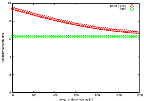
Fig. 3: The neutrino probability in the forward direction per time at a finite distance L is given. The constant shows the short-range normal term and the long-range term is written on top of the normal term. The horizontal axis shows the distance in [m] and the probability is of arbitrary unit. Clear excess is seen in the distance below 1200 [m]. The neutrino mass, pion energy, neutrino energy are 1 [eV/$c^{2}$], 4 [GeV], and 800 [MeV].

5.2 Total transition probability

Adding the slowly decreasing part and the short-range part, we have the final expression of the total probability. The neutrino coordinate ${\vec{X}}_{\nu}$ of the final state is integrated in Eq.($\ref{total-probability2})$ and a factor $({\sigma_{\pi}\pi})^{\frac{3}{2}}$ emerges. This $\sigma_{\pi}$ dependence is cancelled by the $({4\pi/\sigma_{\pi}})^{\frac{3}{2}}$ from the normalization Eq. $(\ref{probability})$ and the final result is independent from $\sigma_{\pi}$. The total transition probability is expressed in the form,

$$P=\text{T}g^{2}m_{\mu}^{2}D_{0}\sigma_{\nu}\int{d^{3}p_{\pi}\over E_{\pi}}\rho_{exp}({\vec{p}}_{\pi})\int{d^{3}p_{\nu}\over E_{\nu}}(p_{\pi}\!\cdot\!p_{\nu})[\tilde{g}(\text{T},\omega_{\nu})+G_{0}],$$

$$D_{0}=|N_{\pi\nu}|^{2}{(\sigma_{\nu}\pi)}^{\frac{3}{2}}{(\sigma_{\pi}\pi)}^{\frac{3}{2}}{1\over(2\pi)^{6}}={1\over(2\pi)^{3}}$$ (129)

where $\text{L}=c\text{T}$ is the length of decay region. Eq. $(\ref{probability-3})$ depends on the neutrino wave packet size $\sigma_{\nu}$.

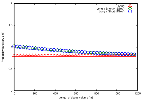
Fig. 4: The total probability integrated in the neutrino angle per time at a finite distance L is given. The constant shows the short-range normal term and the long-range term is written on top of the normal term. The horizontal axis shows the distance in [m] and the probability is of arbitrary unit. The excess becomes less clear than the forward direction, but is seen in the distance below 1200 [m]. The neutrino mass, pion energy, neutrino energy are 1.0 [eV/$c^{2}$], 4 [GeV] and 4.5 [GeV] , and 800 [MeV].

5.2.1 Neutrino angle integration

In the normal term $G_{0}$ of Eq. (129) the cosine of neutrino angle $\theta$ is determined approximately from

$$(p_{\pi}-p_{\nu})^{2}=p_{\mu}^{2}=m_{\mu}^{2},$$ (130)

because the energy and momentum conservation is approximately satisfied in the normal term. Hence the product of the momenta is expressed by the masses

$$p_{\pi}\!\cdot\!p_{\nu}={m_{\pi}^{2}-m_{\mu}^{2}\over 2},$$ (131)

and the cosine of the angle satisfies

$$1-\cos\theta={m_{\pi}^{2}-m_{\mu}^{2}\over 2|\vec{p}_{\pi}||\vec{p}_{\nu}|}-{m_{\pi}^{2}\over 2|\vec{p}_{\pi}|^{2}}.$$ (132)

The $\cos\theta$ is very close to 1. On the other hand, the long-range component of the neutrino probability, $\tilde{g}(\text{T},\omega_{\nu})$ of Eq. (129), is derived from the light-cone singular term. This term is present only when the product of the momenta is in the convergence domain Eq. $({\ref{convergence-condition}})$. Hence the long-range term is present in the kinematical region,

$$|\vec{p}_{\nu}|(E_{\pi}-|\vec{p}_{\pi}|)\leq p_{\pi}\!\cdot\!p_{\nu}\leq{m_{\pi}^{2}-m_{\mu}^{2}\over 2}.$$ (133)

Since the angular region of Eq. (133) is slightly different from Eq. $(\ref{on-shell-angle})$ and it is impossible to distinguish the latter from the former region experimentally, the neutrino angle is integrated. We integrate the neutrino angle of both terms separately. We have the normal term, $G_{0}$, in the form

$$\int\frac{d\vec{p}_{\nu}}{E_{\nu}}(p_{\pi}\cdot p_{\nu})G_{0}$$

$$\simeq\int\frac{d\vec{p}_{\nu}}{E_{\nu}}(p_{\pi}\!\cdot\!p_{\nu})2\sqrt{\frac{\sigma_{\nu}}{\pi}}\left(\frac{\pi}{\sigma_{\nu}}\right)^{\frac{3}{2}}\int\frac{d\vec{q}}{\sqrt{q^{2}+m_{\mu}}}$$

$$\times\delta\left(E_{\pi}-E_{\nu}-\sqrt{q^{2}+m_{\mu}^{2}}\right)\delta^{(3)}\left(\vec{p}_{\pi}-\vec{p}_{\nu}-\vec{q}\right)\theta\left(E_{\pi}-\sqrt{q^{2}+m_{\mu}^{2}}\right)$$

$$=\left(\frac{1}{\sigma_{\nu}}\right)(2\pi)^{2}\left({m_{\pi}^{2}-m_{\mu}^{2}\over 2}\right){1\over|\vec{p}_{\pi}|}\int_{E_{\nu,min}}^{E_{\nu},max}dE_{\nu},$$ (134)

where

$$E_{\nu,min}={m_{\pi}^{2}-m_{\mu}^{2}\over 2(E_{\pi}+|\vec{p}_{\pi}|)},E_{\nu,max}={m_{\pi}^{2}-m_{\mu}^{2}\over 2(E_{\pi}-|\vec{p}_{\pi}|)}$$ (135)

and the Gaussian function is approximated by the delta function for the computational convenience. The angle is determined uniquely. We have for the long-range term, $\tilde{g}(\text{T},\omega_{\nu})$, in the form

$$\int\frac{d\vec{p}_{\nu}}{E_{\nu}}(p_{\pi}\!\cdot\!p_{\nu})\tilde{g}(\text{T},\omega_{\nu})$$

$$=2\pi\int\frac{|\vec{p}_{\nu}|^{2}d|\vec{p}_{\nu}|}{E_{\nu}}\int_{\frac{E_{\pi}E_{\nu}-\frac{1}{2}(m_{\pi}^{2}-m_{\mu}^{2})}{|\vec{p}_{\pi}||\vec{p}_{\nu}|}}^{1}d\cos\theta(E_{\pi}E_{\nu}-|\vec{p}_{\pi}||\vec{p}_{\nu}|\cos\theta)\tilde{g}(\text{T},\omega_{\nu})$$

$$=2\pi\int\frac{|\vec{p}_{\nu}|^{2}d|\vec{p}_{\nu}|}{E_{\nu}}\left[E_{\pi}E_{\nu}\cos\theta-\frac{1}{2}|\vec{p}_{\pi}||\vec{p}_{\nu}|\cos^{2}\theta\right]_{\frac{E_{\pi}E_{\nu}-\frac{1}{2}(m_{\pi}^{2}-m_{\mu}^{2})}{|\vec{p}_{\pi}||\vec{p}_{\nu}|}}^{1}\tilde{g}(\text{T},\omega_{\nu})$$

$$=2\pi\int_{E_{\nu,min}}^{E_{\nu},max}\frac{dE_{\nu}}{2|\vec{p}_{\pi}|}\left\{\frac{1}{4}\left(m_{\pi}^{2}-m_{\mu}^{2}\right)^{2}-(E_{\pi}E_{\nu}-|\vec{p}_{\pi}||\vec{p}_{\nu}|)^{2}\right\}\tilde{g}(\text{T},\omega_{\nu}),$$ (136)

where the angle is very close to the former value but is not uniquely determined. Finally we have the energy dependent probability

$$\frac{dP}{dE_{\nu}}=\text{T}g^{2}m_{\mu}^{2}D_{0}\int{d^{3}p_{\pi}\over E_{\pi}}\rho_{exp}({\vec{p}}_{\pi})\frac{2\pi}{|\vec{p}_{\pi}|}\times\biggl{[}{\pi}(m_{\pi}^{2}-m_{\mu}^{2})$$

$$+{\sigma_{\nu}\over 2}\left\{\frac{1}{4}\left(m_{\pi}^{2}-m_{\mu}^{2}\right)^{2}-(E_{\pi}E_{\nu}-|\vec{p}_{\pi}||\vec{p}_{\nu}|)^{2}\right\}\tilde{g}(\text{T},\omega_{\nu})\biggr{]}.$$ (137)

5.3 Comparison with measurements

5.3.1 Sharp pion momentum

When initial pion has a discrete momentum ${\vec{P}}_{\pi}$, the $\rho_{exp}({\vec{p}}_{\pi})$ is given as

$$\rho_{exp}({\vec{p}}_{\pi})=\delta({\vec{p}}_{\pi}-{\vec{P}}_{\pi})$$ (138)

and the energy-dependent probability for this pion is

$$\frac{dP}{dE_{\nu}}=\text{T}g^{2}m_{\mu}^{2}D_{0}{1\over E_{\pi}}\frac{2\pi}{|\vec{P}_{\pi}|}\biggl{[}{\pi}(m_{\pi}^{2}-m_{\mu}^{2})$$

$$+{\sigma_{\nu}\over 2}\left\{\frac{1}{4}(m_{\mu}^{2}-m_{\pi}^{2})^{2}-(E_{\pi}E_{\nu}-|\vec{P}_{\pi}||\vec{p}_{\nu}|)^{2}\right\}\tilde{g}(\text{T},\omega_{\nu})\biggr{]}.$$ (139)

Eq. $(\ref{total-probability-energy2})$ is independent from the position ${\vec{X}}_{\pi}$ of the initial state and depends upon the momenta and the time difference $\text{T}=T_{\nu}-T_{\pi}$. Consequently although quantum mechanics tells that the probability Eq.$(\ref{total-probability-energy2})$ should be applied to events of one initial state of the pion, it is possible to average over different positions. The result is obviously the same Eq. $(\ref{total-probability-energy2})$.

At $\text{T}\rightarrow\infty$, $\tilde{g}(\text{T},\omega_{\nu})$ vanishes and the decay rate per time of the energy $E_{\pi}$ is given from the first term of Eq. $(\ref{total-probability-energy2})$ as

$$P/\text{T}=g^{2}m_{\mu}^{2}D_{0}{1\over E_{\pi}}\frac{2\pi}{|\vec{P}_{\pi}|}{\pi}(m_{\pi}^{2}-m_{\mu}^{2})\int_{E_{\nu,min}}^{E_{\nu,max}}dE_{\nu}$$

$$=g^{2}m_{\mu}^{2}{1\over 4\pi}\frac{m_{\pi}^{2}}{E_{\pi}}\left(1-{m_{\mu}^{2}\over m_{\pi}^{2}}\right)^{2}.$$ (140)

The stationary value is independent from the wave packet size and is consistent with [21]. This value furthermore agrees to the standard value obtained using the plane waves. Hence the large time limit of our result is equivalent to the known result.

At finite T, the diffraction term does not vanish and Eq. $(\ref{total-probability-energy2})$ deviates from the standard value obtained using the plane waves. The relative magnitude of the diffraction term $\tilde{g}(\text{T},\omega_{\nu})$ to the normal term $G_{0}$ is independent from detection process. So we compute $\tilde{g}(\text{T},\omega_{\nu})$ and $G_{0}$ of Eq. (129) at the forward direction $\theta=0$ and the energy dependent total probability that is integrated over the neutrino angle in the following.

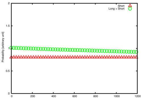
Fig. 5: The total probability integrated in the neutrino angle per time at a finite distance L is given. The constant shows the short-range normal term and the long-range term is written on top of the normal term. The horizontal axis shows the distance in [m] and the probability is of arbitrary unit. Clear uniform excess is seen in the distance below 1200 [m]. The neutrino mass, pion energy, neutrino energy are 0.6 [eV/$c^{2}$], 4 [GeV], and 800 [MeV].

The function $\tilde{g}(\text{T},\omega)$ and $G_{0}$ are plotted in Fig. 3 for the mass of neutrino, $m_{\nu}=1\,[\text{eV}/c^{2}]$, the pion energy $E_{\pi}=4$ [GeV], and the neutrino energy $E_{\nu}=800$ [MeV]. For the wave packet size of the neutrino, the size of the nucleus of the mass number $A$, $\sigma_{\nu}=A^{\frac{2}{3}}/m_{\pi}^{2}$ is used. The value becomes $\sigma_{\nu}=6.4/m_{\pi}^{2}$ for the ¹⁶O nucleus and this is used for the following evaluations. From this figure it is seen that there is an excess of the flux at short distance region $\text{L}<600$ [m] and the maximal excess is about $0.4$ at $\text{L}=0$. The slope at the origin $\text{L}=0$ is determined by $\omega_{\nu}$. The slowly decreasing term that is generated from the singularity at the light cone has a finite magnitude.

The total probability that is integrated over the neutrino angle Eq. $(\ref{total-probability-energy})$ is presented next. The probability for the neutrino mass $m_{\nu}=1.0\,[\text{eV}/c^{2}]$ and the pion energy $4$ [GeV] and $4.5$ [GeV] are given in Fig. 4, and for the smaller neutrino mass $m_{\nu}=0.6\,[\text{eV}/c^{2}]$ is given in Fig. 5. $G_{0}$ is unchanged with the distance but the long-distance term, $\tilde{g}(\text{T},\omega_{\nu})$, decreases slowly with the distance than that of $m_{\nu}=1\,[\text{eV}/c^{2}]$. Hence the longer distance is necessary if the mass of the neutrino is even smaller. For the muon neutrino, it is impossible to measure the event at a energy lower than few $100$ [MeV]. The electron neutrino is used then. Considering the situation for the electron neutrino, we present the total probability for the lower energies. The probability for the neutrino mass $m_{\nu}=1.0\,[\text{eV}/c^{2}]$ with the energy $100$ [MeV] is given in Fig. 6. The slowly decreasing component of the probability becomes more prominent with lower values. Hence to observe this component, the experiment of the lower neutrino energy is more convenient.

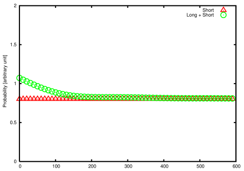
Fig. 6: The total probability integrated in the angle per time at a finite distance L is given. The constant shows the short-range normal term and the long-range term is written on top of the normal term. The horizontal axis shows the distance in [m] and the probability is of arbitrary unit. Clear excess and decreasing behavior are seen in the distance below 600 [m]. The neutrino mass, pion energy, neutrino energy are 1 [eV/$c^{2}$], 4 [GeV], and 100 [MeV].

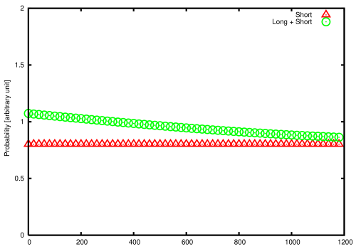
Fig. 7: The neutrino probability integrated in the neutrino angle per time at a finite distance L is given. The constant shows the short-range normal term and the long-range term is written on top of the normal term. The horizontal axis shows the distance in [m] and the probability is of arbitrary unit. Clear excess is seen in the distance below 1200 [m]. The neutrino mass, pion energy, neutrino energy are 0.1 [eV/$c^{2}$], 4 [GeV], and 10 [MeV].

The typical length $\text{L}_{0}$ of the diffraction term is

$$\text{L}_{0}~{}[\text{m}]={2E_{\nu}\hbar c\over m_{\nu}^{2}}=400{E_{\nu}[\text{GeV}]\over m_{\nu}^{2}[\text{eV}^{2}/c^{4}]}.$$ (141)

By the observation of this component together with the neutrino’s energy, the determination of the neutrino mass may becomes possible. The neutrino’s energy is measured with uncertainty $\Delta E_{\nu}$, which is of the order $0.1\times E_{\nu}$. This uncertainty is $100$ [MeV] for the energy $1$ [GeV] and is accidentally same order as that of the minimum uncertainty $\hbar/\delta x$ derived from Eq. $(\ref{mfp-neutrino-N})$. The total probability for a larger value of energy uncertainty is easily computed using Eq. (129). Figs. (3)-(7) show the length dependence of the probability. If the mass is around $1\,[\text{eV}/c^{2}]$ the excess of the neutrino flux of about $20$ percent at the distance less than a few hundred meters is found. In the long-baseline neutrino oscillation experiments, the neutrino flux at the near detectors has observed excesses of about $10-20$ percent [28, 29, 30]. We believe this is connected with the excesses found in this paper. We use mainly $m_{\nu}=1\,[\text{eV}/c^{2}]$ throughout this paper.

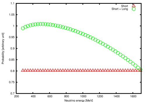
Fig. 8: The energy dependence of the probability integrated in the angle at distance $\text{L}=100$ [m] is given. The lower curve shows the short-range normal term and the long-range term is added on top of the normal term. The horizontal axis shows the neutrino energy in [MeV] and the probability is of arbitrary unit. The neutrino mass and pion energy are 1.0 [eV/$c^{2}$] and 4 [GeV].

Because the probability has a constant term and the T-dependent term, the T-dependent term is extracted easily by subtracting the constant term from the total probability. The slowly decreasing component decreases with the scale determined by the neutrino’s mass and the energy. Although the excess of the flux would be found, the decreasing behavior becomes difficult to observe if the mass is less than $0.1\,[\text{eV}/c^{2}]$ for the muon neutrino. In this case, the electron neutrino is useful. The electron neutrino is produced in the decays of the muon, neutron, K-meson, and nucleus. In these decays the present mechanism works. So we plot the figure for $m_{\nu}=0.1\,[\text{eV}/c^{2}]$, $E_{\nu}=10\,[\text{MeV}]$ in Fig. 7. A decreasing part is clearly seen. So in order to observe the slow decreasing behavior for the small neutrino mass less than or about the same as $0.1\,[\text{eV}/c^{2}]$, the electron neutrino should be used. The decay of the muon and others will be studied in a forthcoming paper. In Fig. 8 the energy dependence of the total probability is given. The long-range term has a different form and has a maximum at the neutrino energy $E_{\nu}\approx{1/3E_{\nu,max}}$.

5.3.2 Wide distribution of pion momentum

When the momentum distribution $\rho_{exp}({\vec{p}}_{\pi})$ of the initial pion is known, the energy-dependent probability of the neutrino is given by Eq. $(\ref{total-probability-energy})$. Eq. $(\ref{total-probability-energy})$ is also independent from the position ${\vec{X}}_{\pi}$ and depends upon the momentum of the pion and of the neutrino and the time difference $\text{T}=T_{\nu}-T_{\pi}$. In the experiments, the pion’s position is not measured and the average over the position is made. This average probability agrees to Eq.$(\ref{total-probability-energy})$. The probability varies slowly with the pion’s momentum and is regarded constant in the energy range of order $100$ [MeV]. So the experimental observation of the diffraction term is quite easy.

5.4 On the universality of the long-distance correction

The long-distance correction of the neutrino detection probability was obtained using the wave packets. The correction is decreasing extremely slowly with the distance. The slope is determined only from the mass and energy of the neutrino and is independent from details of other parameters of the system such as the size or shape of the wave packets and the position of the final wave packets and others. Hence this is the genuine property of the wave function $|\text{muon,~{}neutrino}(t)\rangle$, of Eq. $(\ref{state-vector})$. The slope of this term has the universal property and is capable of measuring in experiments.

5.4.1 Muon in pion decay

When the muon is observed in the same processes, the anomalous behavior is determined by the mass and energy of the muon as ${m_{\mu}^{2}/2E_{\mu}}$. Since the muon mass is larger than the neutrino mass by $10^{8}$, the typical length for the muon is smaller than that of the neutrino by $10^{-16}$. For the muon of energy 1 $[\text{GeV}]$, the length is order $10^{-12}$ [m]. This value is a microscopic size. So the muon probability becomes constant in this distance and has no observable long-range effect. The muon from the pion decay has no coherence effect and can be treated incoherently.

6 Summary and implications

In this paper, we studied the interference of the neutrino in high energy pion decay. The position-dependent neutrino flux was computed and the new long-distance component of universal property that is insensitive to the pion’s initial conditions was found to exist in addition to the normal in-coherent term. The pion’s coherence length estimated in Section 2 shows that this is long enough for the new universal term to be observed. Since the new term reflects the interference of the neutrino, it decreases with the distance in the universal manner that depends upon the absolute value of the neutrino mass.

The present interference phenomenon is caused by the light-cone singularity of the correlation function of the pion and muon system $\Delta_{\pi,\mu}(\delta t,\delta\vec{x})$ and the slow phase $\bar{\phi}_{c}$ of the neutrino wave function, Eq. $(\ref{light-phase})$ These two ingredients are characteristic phenomena of the relativistic invariant system. The light-cone singularity is formed from the waves of the infinite momentum, which have always the light velocity. The slow phase of the neutrino wave packet is the outcome of the cancellation between the time and space oscillations. The phase is determined by the difference of space-time coordinates $(\delta t,\delta{\vec{x}})$ and the central values of the energy and momentum, as ${E({\vec{p}}\,)\delta t-{\vec{p}}\!\cdot\!\delta{\vec{x}}}$, where the energy $E({\vec{p}}\,)$ is given by $\sqrt{{\vec{p}}^{\,2}+m^{2}}$. When the difference of positions $\delta{\vec{x}}$ is moving with the light velocity in the parallel direction to the momentum ${\vec{p}}$, ${\vec{v}}_{c}=c({\vec{p}}/p)$, as $\delta{\vec{x}}={\vec{v}}_{c}\delta t$, then the total phase becomes $E_{\nu}\delta t-{\vec{p}}_{\nu}\!\cdot\!\delta{\vec{x}}=(m_{\nu}^{2}/2E_{\nu})\delta t$. The angular velocity becomes the small value $m_{\nu}^{2}/2E_{\nu}$ due to the relativistic invariance and makes the interference phenomenon long-range. The new term in the probability decreases slowly with the distance in the universal manner determined by the mass and energy of the neutrino as $m_{\nu}^{2}/2E_{\nu}$. This form is independent from the details of wave packet shape and parameters as far as the reality of the neutrino wave function $\tilde{w}({\vec{x}})$ is satisfied, which is ensured from the invariance under the time inversion. The relative magnitude of this component is not universal and depends upon the size of wave packet. Based on the estimation of the size, we found that the magnitude of the new universal term is sizable for the measurement. Since the slope of the probability, Eq. $(\ref{probability-3})$, is determined by the mass and energy of the neutrino, the absolute value of the neutrino mass would be found from the neutrino interference experiments.

The new component shall be observed as the excesses of the neutrino flux in the ground experiments. The excesses of the neutrino flux at the macroscopic short distance region of the order of a few hundred meters were computed and shown in Figs. (3)-(8). From these figures, the excesses are not large but are sizable magnitudes. Hence these excesses shall be observed in these distances. Actually fluxes measured in the near detectors of the long-baseline experiments of K2K [28] and MiniBooNE [29] may show excesses of about $10-20$ percent of the Monte Carlo estimations. Monte Carlo estimations of the fluxes are obtained using naive decay probabilities and do not have the coherence effects we presented in the present work. So the excess of these experiments may be related with the excesses due to interferences. The excess is not clear in MINOS [30]. With more statistics, qualitative analysis might become possible to test the new universal term on the neutrino flux at the finite distance. From Figs. (3)-(8), if the mass is in the range from $0.1\,[\text{eV}/c^{2}]$ to $2\,[\text{eV}/c^{2}]$, the near detectors at T2K, MiniBooNE, MINOS and other experiments might be able to measure these signatures. The absolute value of the mass could be found then. It is worthwhile at the end to summarize the reasons why the interference term of the long-distance behavior emerges in the pion decay and is computed with the wave packet representation. The connection of the long-distance interference phenomenon of the neutrino with the Heisenberg’s uncertainty relation is also addressed here.

Due to relativistic invariance, the correlation function $\Delta_{\pi,\mu}(\delta t,\delta\vec{x})$ has a singularity near $\lambda=0$, which is extended to large distance $|\delta{\vec{x}|}\rightarrow\infty$, as was shown in Eq. (82). This is one of the features of relativistic quantum fields and is one reason why the long-range correlation emerged. For a non-relativistic system, on the other hand, the same calculation for stationary states is made by,

$$\int d{\vec{k}}\langle{\vec{x}}_{1}|{\vec{k}}\rangle\langle{\vec{k}}|{\vec{x}}_{2}\rangle=\delta({\vec{x}}_{1}-{\vec{x}}_{2}),$$ (142)

and the only one point $\delta{\vec{x}}=0$ satisfies the condition. Long-range correlation is not generated. The rotational invariant three-dimensional space is compact but the Lorentz invariant four-dimensional space is non-compact. So it is quite natural for the non-relativistic system not to have the long-range correlation that the relativistic system has. The light-cone singularity is the peculiar property of the relativistic system.

Heisenberg uncertainty relation is slightly modified in the wave along the light cone. The neutrino wave function behaves at large-distance along the light-cone region in the form

$$\psi_{\nu}(t,{\vec{x}})=f{e^{i(E_{\nu}t-{\vec{p}}_{\nu}\cdot{\vec{x}})}\over x}=f{e^{i{m_{\nu}^{2}\over 2E_{\nu}}t}\over ct},$$ (143)

where $f$ has no dependence on the distance $|\vec{x}|$. Consequently the uncertainty relation between the energy width $\delta E$ and the time interval $\delta t$ becomes

$$\delta t\delta{m_{\nu}^{2}\over 2E_{\nu}}=\delta t\delta E\times{1\over 2}\left({m_{\nu}\over E_{\nu}}\right)^{2}\approx\hbar.$$ (144)

The ratio $({m_{\nu}/E_{\nu}})^{2}$ is of the order $10^{-18}$ and $\delta t$ becomes macroscopic even if the energy width $\delta E$ is microscopic of order 100 [MeV]. For instance if the pion Compton wave length, $\lambda_{\pi}$, is used for the microscopic length, then $c\delta t$ becomes

$$10^{18}\times\lambda_{\pi}\approx 10^{3}m,$$ (145)

which is about the distance between the pion source and the near detector in fact. So interference effect of the present paper appears in this distance and is observable using the apparatus of much smaller size.

The position-dependent probability was computed easily with the use of the wave packet representation. Any representation is equivalent to plane waves as far as the whole complete set of functions is used. The ordinary probability of the transition process is defined from the states at $t=\pm\infty$. The normal scattering amplitude is the overlap between the in-state at $t=-\infty$ and out-state at $t=\infty$, and the space-time coordinates are integrated from $-\infty$ to $\infty$ and the energy and momentum of the final state is the same as that of the initial state. Hence in the pion decay, the momentum of the muon in the final state of the ordinary scattering experiments are bounded. So the infinite momentum is not included in the muon of the final state. From these amplitudes, the amplitudes and probability at the finite-time interval are neither computable nor obtained. In the wave packet formalism, on the other hand, it is possible to compute the amplitude and probability at finite-time interval directly. Energy and momentum conservation is slightly violated in this amplitude and the states of infinite momentum couple and give the light-cone singularity to the correlation function $\Delta_{\pi,\mu}({\delta x})$. The contribution from these states vanishes at infinite time and these states do not contribute to the probability measured at infinite distance, i.e., ordinary S-matrix. Thus the light-cone singularity gave the interference term, which ended up as the finite-time interval effect of the neutrino probability. Wave packet formalism gives new information that is not calculable in the standard scattering amplitude. Hence our calculation does not contradict with the ordinary calculation of the S-matrix in momentum representation but has advantage of giving a new universal physical quantity directly.

Since characteristic small phase of the relativistic wave along the light cone and the light-cone singularity are derived from Lorentz invariance, there would be similar effect if there exists other light particle. Axion is a possible candidate of light particle and might show the long-distance interference phenomenon.

In this paper we ignored higher order effects such as pion life time and pion mean free path in studying the quantum effects. We will study these problems and other large scale physical phenomena of low energy neutrinos in subsequent papers.

Appendix Appendix A Light-cone singularity

A-I Light-cone singularity and small neutrino mass

A conjugate momentum to $(\delta t,\delta{\vec{x}})$ is $p_{\pi}-p_{\mu}$ from Eq. $(\ref{pi-mucorrelation})$ and the invariant square of this momentum becomes

$$(p_{\pi}-p_{\mu})^{2}=m_{\pi}^{2}+m_{\mu}^{2}-2\left(\sqrt{\vec{p}_{\pi}^{\,2}+m_{\pi}^{2}}\right)\left(\sqrt{\vec{p}_{\mu}^{\,2}+m_{\mu}^{2}}\right)+2|\vec{p}_{\pi}||\vec{p}_{\mu}|\cos\theta,$$ (146)

where $\theta$ is the angle between the pion and muon momenta. The invariant vanishes when the cosine of angle becomes

$$\cos\theta_{c} ={-m_{\pi}^{2}-m_{\mu}^{2}+2\left(\sqrt{\vec{p}_{\pi}^{\,2}+m_{\pi}^{2}}\right)\left(\sqrt{\vec{p}_{\mu}^{\,2}+m_{\mu}^{2}}\right)\over 2|\vec{p}_{\pi}||\vec{p}_{\mu}|}$$

$$=1-{{m_{\pi}}^{2}\over 2|\vec{p}_{\pi}||\vec{p}_{\mu}|}\left(1-{|\vec{p}_{\mu}|\over|\vec{p}_{\pi}|}\right)-{{m_{\mu}}^{2}\over 2|\vec{p}_{\pi}||\vec{p}_{\mu}|}\left(1-{|\vec{p}_{\pi}|\over|\vec{p}_{\mu}|}\right)+\text{ small~{} terms}.$$ (147)

This equation has a solution in a finite muon momentum region for a given pion momentum.

A-II Long-range correlation for general wave packets

A-II.1 Non-Gaussian wave packet

Non-Gaussian wave packets were studied in the general manner in the text and the universal behavior of the phase was obtained. In this appendix the explicit forms of the wave packets are studied. It is reconfirmed that the long-range component of the probability at around $t={2\pi E_{\nu}/m_{\nu}^{2}}$ becomes the universal form.

type 1

One way to express the non-Gaussian wave packet is to multiply Hermitian polynomials and to write the amplitude in the form

$$\frac{N_{\nu}}{(2\pi)^{\frac{3}{2}}}\int d{\vec{k}}_{\nu}e^{-{\sigma_{\nu}\over 2}({\vec{k}}_{\nu}-{\vec{p}}_{\nu})^{2}}H_{n}(\sqrt{\sigma_{\nu}}({\vec{k}}_{\nu}-{\vec{p}}_{\nu}))e^{i\left(E({\vec{k}}_{\nu})(t-T_{\nu})-{\vec{k}}_{\nu}\cdot({\vec{x}}-{\vec{X}}_{\nu})\right)}.$$ (148)

where $H_{n}$ is assumed to be real in order the wave packets to preserve the time reversal symmetry and an even function of ${\vec{k}_{\nu}}-{\vec{p}}_{\nu}$ in order the wave packets to preserve parity , Eqs.  $(\ref{time-reversal})$ and $(\ref{parity})$.

Since we study symmetric wave packets, it is sufficient to prove the simplest case

$$H_{n}={\sigma_{\nu}}({\vec{k}}_{\nu}-{\vec{p}}_{\nu})^{2}.$$ (149)

The spreading effect was studied in the previous appendix and does not change the final result. So we ignore the spreading effect here. The momentum integration Eq. $(\ref{amplitude})$ is replaced with

$$\int d{\vec{k}}_{\nu}e^{-{\sigma_{\nu}\over 2}({\vec{k}}_{\nu}-{\vec{p}}_{\nu})^{2}}\sigma_{\nu}({\vec{k}}_{\nu}-{\vec{p}}_{\nu})^{2}e^{i(E({\vec{k}}_{\nu})(t-T_{\nu})-{\vec{k}}_{\nu}\cdot({\vec{x}}-{\vec{X}}_{\nu}))}.$$ (150)

After the straightforward calculations we have this integral in the form,

$$\sigma_{\nu}e^{i(E({\vec{p}}_{\nu})(t-T_{\nu})-{\vec{p}}_{\nu}\cdot({\vec{x}}-{\vec{X}}_{\nu}))-{1\over 2\sigma_{\nu}}({\vec{x}}-{\vec{X}}_{\nu}-{\vec{v}}_{\nu}(t-T_{\nu}))^{2}}\int d{\vec{k}}_{\nu}e^{-{\sigma_{\nu}\over 2}\left({\vec{k}}_{\nu}-{\vec{p}}_{\nu}+{i\over\sigma_{\nu}}\{{\vec{x}}-{\vec{X}}_{\nu}-{\vec{v}}_{\nu}(t-T_{\nu})\}\right)^{2}}$$

$$\times\Biggr{[}\left({\vec{k}}_{\nu}-{\vec{p}}_{\nu}+{i\over\sigma_{\nu}}\{{\vec{x}}-{\vec{X}}_{\nu}-{\vec{v}}_{\nu}(t-T_{\nu})\}\right)^{2}-{1\over\sigma_{\nu}^{2}}\{{\vec{x}}-{\vec{X}}_{\nu}-{\vec{v}}_{\nu}(t-T_{\nu})\}^{2}$$

$$+{2i\over\sigma_{\nu}}\left({\vec{k}}_{\nu}-{\vec{p}}_{\nu}+{i\over\sigma_{\nu}}\{{\vec{x}}-{\vec{X}}_{\nu}-{\vec{v}}_{\nu}(t-T_{\nu})\}\right)\{{\vec{x}}-{\vec{X}}_{\nu}-{\vec{v}}_{\nu}(t-T_{\nu})\}\Biggr{]}$$

$$=\left({2\pi\over\sigma_{\nu}}\right)^{\frac{3}{2}}e^{i(E({\vec{p}}_{\nu})(t-T_{\nu})-{\vec{p}}_{\nu}\cdot({\vec{x}}-{\vec{X}}_{\nu}))-{1\over 2\sigma_{\nu}}({\vec{x}}-{\vec{X}}_{\nu}-{\vec{v}}_{\nu}(t-T_{\nu}))^{2}}$$

$$~{}~{}~{}\times\left(3-{1\over\sigma_{\nu}}\{{\vec{x}}-{\vec{X}}_{\nu}-{\vec{v}}_{\nu}(t-T_{\nu})\}^{2}\right).$$ (151)

Next the integral Eq. (88) is studied. This becomes for the non-Gaussian wave packet to the integral

$$\tilde{J}_{\delta({\lambda})}=N_{\nu}^{2}\int d{\vec{x}}_{1}d{\vec{x}}_{2}e^{i\phi(\delta x)-{1\over 2\sigma_{\nu}}({\vec{x}}_{1}-{\vec{X}}_{\nu}-{\vec{v}}_{\nu}(t_{1}-T_{\nu}))^{2}-{1\over 2\sigma_{\nu}}({\vec{x}}_{2}-{\vec{X}}_{\nu}-{\vec{v}}_{\nu}(t_{2}-T_{\nu}))^{2}}{1\over 4\pi}\delta(\lambda)$$

$$\times\left(3-{1\over\sigma_{\nu}}\{{\vec{x}}_{1}-{\vec{X}}_{\nu}-{\vec{v}}_{\nu}(t_{1}-T_{\nu})\}^{2}\right)\left(3-{1\over\sigma_{\nu}}\{{\vec{x}}_{2}-{\vec{X}}_{\nu}-{\vec{v}}_{\nu}(t_{2}-T_{\nu})\}^{2}\right),$$ (152)

and is written by using the center coordinate ${X}^{\mu}={{x}_{1}^{\mu}+{x}_{2}^{\mu}\over 2}$ and relative coordinate ${r}^{\mu}={x}_{1}^{\mu}-{x}_{2}^{\mu}$ in the form

$$N^{2}\int d{\vec{X}}d{\vec{r}}e^{i\phi(\delta x)-{1\over\sigma_{\nu}}\tilde{\vec{X}}^{2}-{1\over{4\sigma_{\nu}}}\tilde{\vec{r}}^{\,2}}{\delta(\lambda)\over 4\pi}$$

$$\ \ \ \times\Biggl{[}9-{3\over\sigma}\left(2\tilde{\vec{X}}^{2}+\frac{1}{2}\tilde{\vec{r}}^{\,2}\right)+\frac{1}{\sigma_{\nu}^{2}}\left(\tilde{\vec{X}}^{4}-\frac{1}{2}\tilde{\vec{X}}^{2}\tilde{\vec{r}}^{\,2}+\frac{1}{16}\tilde{\vec{r}}^{\,4}\right)\Biggr{]},$$ (153)

where

$$\tilde{\vec{X}}={\vec{X}}-{\vec{X}}_{\nu}-{\vec{v}}_{\nu}(X^{0}-T_{\nu}),\ \tilde{\vec{r}}={\vec{r}}-{\vec{v}}r^{0}.$$

The integration on ${\vec{X}}$ and ${\vec{r}}$ are made and we have the final result

$$\tilde{J}_{\delta({\lambda})} =N_{\nu}^{2}(\sigma_{\nu}\pi)^{\frac{3}{2}}\sigma_{\nu}{1\over 2r^{0}}e^{i(E-p_{\nu})r^{0}}$$

$$\ \ \times\left[-{13\over 4}+{9\over 4}{1\over\sigma_{\nu}}(1-v_{\nu})^{2}(r^{0})^{2}+O((1-v_{\nu})^{4}(r^{0})^{4})\right].$$ (154)

Thus the phase factor has the same universal form as the Gaussian wave packet and the correction is determined by the small parameter $(1-v_{\nu})^{2}(r^{0})^{2}$ in the form

$${1\over\sigma_{\nu}}(1-v_{\nu})^{2}(r^{0})^{2}=\left({1\over E_{\nu}\sigma_{\nu}}\right)^{2}\left({m_{\nu}^{2}\over 2E_{\nu}}r^{0}\right)^{2},$$ (155)

hence the correction is negligible at high energy.

We have proved that the correlation function of the non-Gaussian wave packet has the same slow phase and long-range term as the Gaussian wave packet and the small correction becomes negligible for the simplest case Eq. 149. Hence for any polynomials $H_{n}$ that are invariant under the time and space inversions, the correlation function has the same long-range term and small negligible corrections.

type 2

Another way to write the non-Gaussian wave packet is to use a function $\alpha({\vec{p}}\,)$, and to write

$$\frac{N_{\nu}}{(2\pi)^{\frac{3}{2}}}\int d{\vec{k}}_{\nu}e^{-\alpha({\vec{k}}_{\nu})+i\left(E({\vec{k}}_{\nu})(t-T_{\nu})-{\vec{k}}_{\nu}\cdot({\vec{x}}-{\vec{X}}_{\nu})\right)}.$$ (156)

The large $t=T$ behavior is found by the stationary momentum which satisfies the equation

$${\partial\over\partial k_{\nu,i}}\alpha|_{{\vec{k}}_{\nu}={\vec{p}}_{\nu}}=0.$$ (157)

Symmetric real wave packet is assumed also here from parity and time reversal invariances of the wave packets and we write,

$$\alpha({\vec{k}}_{\nu})=\alpha({\vec{p}}_{\nu})+{({\vec{k}}_{\nu}-{\vec{p}}_{\nu}\,)^{2}\over 2}\sigma_{\nu}+(k_{\nu}-p_{\nu})_{i}^{2}(k_{\nu}-p_{\nu})_{j}^{2}C{ij}+\cdots,$$ (158)

where the $\sigma$ and $C_{ij}$ are real numbers. The momentum integration of Eq. $(\ref{non-gaussian-alpha})$ becomes the form

$$\frac{N^{\prime}_{\nu}}{(2\pi)^{\frac{3}{2}}}\int d{\vec{k}}_{\nu}e^{-{\sigma_{\nu}\over 2}({\vec{k}}_{\nu}-{\vec{p}}_{\nu})^{2}+i\left(E({\vec{k}}_{\nu})(t-T_{\nu})-{\vec{k}}_{\nu}\cdot({\vec{x}}-{\vec{X}}_{\nu})\right)}e^{-(((k_{\nu}-p_{\nu})_{i})^{2}((k_{\nu}-p_{\nu})_{j})^{2}C{ij})}$$

$$=\frac{N^{\prime}_{\nu}}{(2\pi)^{\frac{3}{2}}}\int d{\vec{k}}_{\nu}e^{-{\sigma_{\nu}\over 2}({\vec{k}}_{\nu}-{\vec{p}}_{\nu})^{2}+i\left(E({\vec{k}}_{\nu})(t-T_{\nu})-{\vec{k}}_{\nu}\cdot({\vec{x}}-{\vec{X}}_{\nu})\right)}$$

$$\times(1-((k_{\nu}-p_{\nu})_{i})^{2}((k_{\nu}-p_{\nu})_{j})^{2}C{ij}).$$ (159)

The correction to the Gaussian wave packet is generated by the higher order terms of ${\vec{k}}_{\nu}-{\vec{p}}_{\nu}$ in the right hand side and is treated in a same way as the previous type 1 case. Hence this integral has the leading long-range term which is equivalent to that of the Gaussian wave packet and the negligible correction expressed by Eq. $(\ref{non-gaussian-correction})$.

For studying the asymptotic behavior at $t-T_{\nu}\rightarrow\infty$ we solve the stationarity equation,

$${\partial\over\partial k_{\nu,i}}\left[\alpha({\vec{k}}_{\nu})-i\{E({\vec{k}}_{\nu})(t-T_{\nu})-{\vec{k}}_{\nu}\cdot({\vec{x}}-{\vec{X}}_{\nu})\}\right]=0$$ (160)

and expand the integral around the stationary momentum. The wave in the transverse direction to this momentum spreads but spreading is very small in the longitudinal direction [10]. From the result of the previous appendix, the final result is the same and so is not presented here.

$\bf type~{}3$

In the type 1 and 2 the time reversal and parity symmetries are assumed for the wave packet shape. If these symmetries are not required, the function $H_{n}$ or $\alpha$ has an imaginary part. In this case, the correlation function has a correction term in the order $(1-v)(t_{1}-t_{2})$ and this term is expressed

$$(1-v_{\nu})(t_{1}-t_{2})={1\over E_{\nu}}{m_{\nu}^{2}\over 2E_{\nu}}(t_{1}-t_{2})$$ (161)

hence the correction term vanishes at the high energy. With a suitable parameter, the universal form of the slowly decreasing component of the probability of the present work may become observable even in arbitrary system. The Lorentz invariant form of the energy dependent phase of the wave packet and the light-cone singularity of the pion and muon decay vertex give this universal behavior.

References

- [1] J. Hosaka, et al, Phys. Rev. Vol. D74, 032002, (2006).
- [2] The Super-Kamiokande Collaboration. Phys. Lett. B539, 179, (2002).
- [3] S. N. Ahmed, et al. Phys. Rev. Lett. 92, 181301 (2004).
- [4] T. Araki, et al. Phys. Rev. Lett. 94, 081801 (2005).
- [5] E. A. Litvinovich. Phys. Atom. Nucl. 72, 522–528 (2009).
- [6] E. Aliu, et al. Phys. Rev. Lett. 94, 081802 (2005).
- [7] K. Nakamura et al. [Particle Data Group], J. Phys. G 37, 075021 (2010).
- [8] C. Weinheimer, et al. Phys. Lett. B460, 219–226 (1999).
- [9] E. Komatsu, et al. Astrophys. J. Suppl. 180, 330–376 (2009).
- [10] K. Ishikawa and T.Shimomura, Prog. Theor. Physics. 114, (2005), 1201-1234.
- [11] K. Ishikawa and Y. Tobita, Prog. Theor. Physics. 122, (2009), 1111-1136.
- [12] K. Ishikawa and Y. Tobita, arXiv:0801.3124 “ Neutrino mass and mixing ” in the 10th Inter. Symp. on “ Origin of Matter and Evolution of Galaxies ” AIP Conf. proc. 1016, P.329(2008)
- [13] M. L. Goldberger and Kenneth M. Watson, Collision Theory (John Wiley & Sons, Inc. New York, 1965).
- [14] R. G. Newton, Scattering Theory of Waves and Particles (Springer-Verlag, New York, 1982).
- [15] J. R. Taylor, Scattering Theory: The Quantum Theory of non-relativistic Collisiions (Dover Publications, New York, 2006).
- [16] T. Sasakawa, Prog. Theor. Physics. Suppl.11, 69(1959).
- [17] B. Kayser, Phys. Rev. D24, 110(1981); Nucl.Phys. B19 (Proc.Suppl), 177(1991).
- [18] C. Giunti, C. W. Kim, and U. W. Lee, Phys. Rev. D44, 3635(1991)
- [19] S. Nussinov, Phys. Lett. B63, 201(1976)
- [20] K. Kiers, S. Nussinov and N. Weiss, Phys. Rev. D53, 537(1996).
- [21] L. Stodolsky, Phys. Rev. D58, 036006(1998).
- [22] H. J. Lipkin, Phys. Lett. B642, 366(2006).
- [23] A. Asahara, K. Ishikawa, T. Shimomura, and T. Yabuki, Prog. Theor. Phys. 113, 385(2005); T. Yabuki and K. Ishikawa, Prog. Theor. Phys. 108, 347(2002).
- [24] The last form of the interaction Hamiltonian is used in the text. If the first expression of using the (V-A) current and the derivative of the pion field is used, the magnitude of the long-distance term is slightly modified.
- [25] A. Tonomura. et al, Ameri. J. Physics. 57 No2, 117(1989).
- [26] A. H. Mueller, Phys. Rev. D12, 2963(1970).
- [27] K. Wilson, in Proceedings of the Fifth International Symposium on Electron and Photon Interactions at High Energies, Ithaca, New York, 1971, p.115 (1971). See also N. N. Bogoliubov and D. V. Shirkov, Introduction to the Theory of Quantized Fields (John Wiley & Sons, Inc. New York, 1976).
- [28] M. H. Ahn, et al, Phys. Rev. Vol. D74, 072003, (2006).
- [29] A. A. Aguilar-Arevalo, et al, Phys. Rev. Vol. D79, 072002, (2009).
- [30] P. Adamson, et al, Phys. Rev. Vol. D77, 072002, (2009).