Wakefield generation in magnetized plasmas

Abstract

We consider wakefield generation in plasmas by electromagnetic pulses propagating perpendicular to a strong magnetic field, in the regime where the electron cyclotron frequency is equal to or larger than the plasma frequency. PIC-simulations reveal that for moderate magnetic field strengths previous results are re-produced, and the wakefield wavenumber spectrum has a clear peak at the inverse skin depth. However, when the cyclotron frequency is significantly larger than the plasma frequency, the wakefield spectrum becomes broad-band, and simultaneously the loss rate of the driving pulse is much enhanced. A set of equations for the scalar and vector potentials reproducing these results are derived, using only the assumption of a weakly nonlinear interaction.

I Introduction

Since the pioneering work in Ref. Tajima-Dawson , where the excitation of a plasma oscillations by a short laser pulse was considered, much interest has been devoted to wakefield generation in plasmas. To a large extent this has been due to the wakefield acceleration concept (see, e.g., Tajima-Dawson ; Kirsanov-1987 ; Phys-reports ; Faure-etal ; Nature-review ; Martins-etal ), where the longitudinal field traveling close to the speed of light in vacuum is used as an effective source for particle acceleration. However, the wakefield properties has also been study from a more theoretical point of view Mironov1990 ; Chen-Alfven ; Multi-wake ; Wadhwani2002 ; Shukla-Hybrid ; PRE1998 . Most studies of wakefield generation has been done for unmagnetized plasmas. This is justified by the fact that in most experiments $\omega_{c}/\omega_{p}\ll 1$, where $\omega_{c}=qB_{0}/m$ is the electron cyclotron frequency, $\omega_{p}=(n_{0}q^{2}/\varepsilon_{0}m)^{1/2}\,$is the plasma frequency   $B_{0}$ is the unperturbed magnetic field strength,  $n_{0}$ is the unperturbed electron density, and $q$ and $m$ is the electron charge and mass respectively. As can be expected, the wakefield properties is not much affected by the magnetic field in this regime. However, for $\omega_{c}/\omega_{p}\gtrsim 1$, and for the exciting source propagating non-parallel to the the external magnetic field, the wakefield is significantly altered by the non-zero $B_{0}$Wadhwani2002 ; Shukla-Hybrid ; PRE1998 ; Yooshii1997 . In particular, as found by e.g. Refs. Yooshii1997 ; PRE1998 , for the EM-pulse traveling perpendicular to the magnetic field, the excited mode becomes an extra-ordinary mode, with a significant electromagnetic part, and a non-zero group velocity.

In the present paper we will re-consider the excitation of the extra-ordinary mode wakefield in a strongly magnetized plasma, allowing for $\omega_{c}/\omega_{p}\gg 1$. In this regime the group-velocity of the wakefield may approach the speed of light in vacuum $c$. In then turns out that the excitation process is significantly altered, as compared to the regime of a more modest value of $B_{0}$. From Particle-In-Cell (PIC) simulations we find that when $B_{0}$ is increased, the wakefield changes from an approximately monochromatic field at low $\omega_{c}/\omega_{p}$, to a broadband one at $\omega_{c}/\omega_{p}\gg 1$. At the same time the energy loss rate of the exciting high-frequency ordinary mode is much increased with increasing $\omega_{c}/\omega_{p}$. A reduced system of equations is derived, generalizing previous Eqs. PRE1998 avoiding the division into fast and slow time scales. The reduced equations are solved numerically, and a good agreement with the full 1D PIC simulations is found.

II PIC-simulations of wake field generation in a magnetized plasma

Here we will study an ordinary mode propagating parallel to an external magnetic field, $\mathbf{B}_{0}=B_{0}\mathbf{x}$. In the absence of the magnetic field, it is well known that the ponderomotive force due to a short electromagnetic pulse will excite a wakefield of electrostatic oscillations Tajima-Dawson ; Kirsanov-1987 . Here we will focus on the effects due to the external magnetic field Yooshii1997 ; PRE1998 . We note that this is more likely to be relevant for experiments in the microwave regime Parchamy2005 , rather than the regime of optical lasers.

The 1D Particle-In-Cell simulation (LPIC++)lpic is carried out to study the effect of external magnetic field on the wakefield generation in magnetized plasma. The typical simulation geometry is shown in Fig. 1, where the exciting electromagnetic (EM) high-frequency pulse is taken to be an ordinary mode. For all the results presented here the EM field amplitude of the ordinary mode driver is considered as 0.2 (in dimensionless unit $a_{0}=eE/m\omega c$, with $\omega$ being the frequency), space and time are taken in units of laser wavelength ($\lambda$) and one laser cycle $\tau=\lambda/c$ respectively. The 800 nm laser with FWHM duration of 8$\tau$ and an initially Gaussian shape propagates through the plasma along the $z$-direction with electric field along $x$ and the laser magnetic field along the $y$-direction NOTE . We have modified the code in order to extend its ability to incorporate the presence of an external magnetic field. The external magnetic field is taken to be along the $x$-direction. The plasma of length 800 $\lambda$ is considered with a 40$\lambda$ of the ramp region at the front. In the ramp region the plasma density increases linearly from 0 to 0.000625 $n_{c}$ (Fig. 1), where $n_{c}=\varepsilon_{0}m\omega^{2}/q^{2}$.

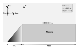
Figure 1: Simulation geometry for the study.

Due to the external magnetic field the wakefield gets both a longitudinal and a transverse part. In Fig. 2 the longitudinal part of the electric field wakefield is shown when varying the value of the external magnetic field. Similarly the transverse component is shown in Fig. 3.

Figure 2: Spatial profiles of the longitudinal wakefield at 600$\tau$ in presence of external magnetic field with ratio $\omega_{c}/\omega_{p}=$ 0.5 (a), 2 (b), 4 (c) and 8 (d) respectively are presented using PIC simulation.

Figure 3: Spatial profiles of the transverse wakefield at 600$\tau$ in presence of external magnetic field with ratio $\omega_{c}/\omega_{p}=$ 0.5 (a), 2 (b), 4 (c) and 8 (d) respectively are presented using PIC simulation.

A number of features from the PIC-simulations agree with the model and results presented in Ref. PRE1998 (see also the discussion and simulation results in Ref. Yooshii1997 )

1. The ratio of the electromagnetic to electrostatic field field amplitude scales as $\omega_{c}/\omega_{p}$ when $B_{0}$ is varied. This is in accordance with the wake field being an extra-ordinary wave mode.

2. By observing the position of the drop in the wake field amplitude, we can deduce that wake field propagates with a group velocity $v_{g\mathrm{wf}}\approx c\omega_{c}^{2}/(\omega_{p}^{2}+\omega_{c}^{2})$, which is in accordance with Refs. Yooshii1997 ; PRE1998

However, there are also some properties of the PIC-simulations that contain new results, as compared to previous findings.

1. The wakefield does have a small but nonzero trailing part at a distance more than $\left(v_{g}-v_{g\mathrm{wf}}\right)T$, where $v_{g}\approx c$ is the group velocity of the ordinary mode, and $T$ is the time after the entrance of the driving pulse. The relative energy content of the wakefield in this tail is larger for larger value of $\omega_{c}/\omega_{p}$.

2. The approximation that the evolution of the wakefield is slow in a frame moving with the pulse is not entirely accurate. Furthermore, the theory of Ref. PRE1998 becomes increasingly inadequate when the magnetic field strength is increased such that $\omega_{c}/\omega_{p}\gg 1$. In particular, Ref. PRE1998 predicts that the loss-rate of the driving pulse is approximately independent of $\omega_{c}/\omega_{p}$. In Fig. 4 the total energy $\propto S_{z}^{WF}+|E_{z}^{2}|$, where $S_{z}^{WF}=|E_{x}B_{y}-E_{x}B_{y}-(B_{x}-B_{0})E_{y}|$ is the EM part, contained in the wakefield is plotted as a function of time for different values of $\omega_{c}/\omega_{p}$. We see that the loss rate of the driving pulse due to the generated wakefield is approximately constant until $\omega_{c}/\omega_{p}\gtrsim 2$, but for larger values of this ratio it increases rapidly.

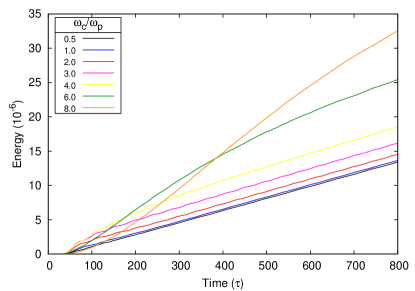
Figure 4: Temporal evolution of the total energy of the wakefield (ES and EM components) for different values of the external magnetic fields using PIC simulation.

One way to understand the deviance from the models in Ref. PRE1998 is to investigate the validity of the basic assumptions. A key ingredient in the derivation is that the evolution should be slow in a frame moving with the group velocity of the driver. A consequence of this is that the phase velocity of the wakefield should match the group velocity of the driver. Since the wakefield is dispersive, such a condition determines the dominating frequency and wavenumber to be excited. Noting that the plasma is underdense with respect to the driver frequency, the group velocity of the driver is close to $c$, which matches the wakefield phase velocity in case the excited wakefield frequency is $\omega_{p}$ and wavenumber $\omega_{p}/c$. Such a condition can be seen to hold for the leading part of the wakefield, but for a strong static field this part actually makes up for a small part of the energy content of the excited extra-ordinary mode. This is illustrated in Fig. 5, where the frequency spectrum of the wakefield is computed as a function of the static magnetic field for a fixed position and time of interaction. For $\omega_{c}/\omega_{p}\gtrsim 2$ we see that the spectrum ceases to peak at $\omega_{p}$, and as a consequence the assumption that the evolution of the wakefield is slow in a system moving with the group velocity cannot be accurate. In the rest of the paper the aim is to investigate the physics of wakefield generation in the regime where the basic equations of Ref. PRE1998 needs to be improved.

III The weakly relativistic 1-D model

For 1D-perturbations (with variations along $z$), the cold relativistic fluid equations can be written.

$$\frac{\partial n}{\partial t}+\frac{\partial}{\partial z}(nv_{z})=0$$ (1)

and

$$\left(\frac{\partial}{\partial t}+v_{z}\frac{\partial}{\partial z}\right)\left(\gamma\mathbf{v-}\frac{q}{m}\mathbf{A}\right)\mathbf{=}\frac{q}{m}\frac{\partial\Phi}{\partial z}\mathbf{z}+\omega_{c}\mathbf{v\times x}$$ (2)

where we have assumed the field to be of the form $\mathbf{E}=-\partial\mathbf{A/}\partial t-\nabla\Phi$, $\mathbf{B}=\nabla\times\mathbf{A+B}_{0}$, the constant magnetic field is $\mathbf{B}_{0}=B_{0}\mathbf{x}$ , $\gamma=(1-v^{2}/c^{2})^{1/2}$ is the relativistic factor, and $\omega_{c}=qB_{0}/m$ is the (constant) cyclotron frequency. For the case where the vector potential was a weakly modulated function, $\mathbf{A=}\widetilde{\mathbf{A}}(z,t)\exp(ikz-\omega t)+\mathrm{c.c.}$, where c.c. stands for complex conjugate, Ref. PRE1998 derived a coupled set for $A$ (with $\widetilde{\mathbf{A}}\mathbf{=}A\mathbf{x}$) and $\Phi$, where $A$ was the vector potential amplitude for the ordinary mode of high-frequency ($\omega\gg\omega_{p}$), and $\Phi$ described the electrostatic potential of the extra-ordinary mode. It was also noted in Ref. PRE1998 that the wake-field was also found to have en electromagnetic part, that could be computed from $\Phi$. The main modification of the wake-field generation due to the static magnetic field $\mathbf{B}_{0}$ was to introduce an electromagnetic component of the wake field, which in turn resulted in a non-zero group velocity. The PIC-simulations of the previous section confirms that these properties are essential ingredients when the external magnetic field is introduced. However, when the ratio $\omega_{c}/\omega_{p}$ is increased beyond unity, we also saw that additional features were introduced. In particular, the assumption of Ref. PRE1998 that the fields evolve slowly in a frame moving with the group velocity, becomes less accurate with increasing value of $\omega_{c}/\omega_{p}$. In the rest of this section we will derive the coupled equations for an extra-ordinary mode driven by an ordinary mode, without any additional assumptions than those of an 1D geometry and a weak nonlinearity. In particular, we will avoid making a WKB-ansatz for the high-frequency ordinary mode. We use the Coulomb gauge and write the vector potential as $\mathbf{A=}A\mathbf{x+}A_{w}\mathbf{y}$. Thus the component $A_{w}$ is associated with the electromagnetic component of the nonlinearly driven extra-ordinary mode, and $\Phi$ with its electrostatic component. The fields of the ordinary mode is derived solely from $A$.

From the $x$-component of the momentum equation (2) we obtain

$$v_{x}=-\frac{qA}{mc}\left(1-\frac{q^{2}A^{2}}{2m^{2}c^{2}}\right)$$ (3)

which we substitute into Ampere’s law, to give

$$\frac{\partial^{2}A}{\partial t^{2}}-c^{2}\frac{\partial^{2}A}{\partial z^{2}}+\omega_{p}^{2}A+\frac{q^{2}}{\varepsilon_{0}m}\delta nA-\frac{\omega_{p}^{2}q^{2}}{2m^{2}c^{4}}A^{3}=0$$ (4)

where $\omega_{p}=(n_{0}q^{2}/\varepsilon_{0}m)^{1/2}$ is the plasma frequency associated with the unperturbed electron density $n_{0}$. Next we study the z-component of the momentum equation. We keep variables that are linear in the extra-ordinary wave-mode, and include quadratic nonlinearities in the ordinary wave mode variables. Essentially this nonlinearity turns out to be the ponderomotive force, but keeping also the second-harmonic term in addition to the low-frequency contribution. The z-component of the velocity is then expressed in terms of the electrostatic potential (through the z-component of Ampere’s law) and the ordinary variables are expressed in terms of $A$. Finally the y-component of the velocity is expressed in terms of $A_{w}$ (from the $y$-component of Ampere’s law). The equation is then expressed solely in terms of the potentials, and we obtain

$$\left(\frac{\partial^{2}}{\partial t^{2}}+\omega_{p}^{2}\right)\frac{\partial\Phi}{\partial z}+\frac{\omega_{c}}{c}\left[\frac{\partial^{2}}{\partial t^{2}}-c^{2}\frac{\partial^{2}}{\partial z^{2}}\right]A_{w}=-\frac{\omega_{p}^{2}q}{2mc^{2}}\frac{\partial A^{2}}{\partial z}.$$ (5)

Finally, we study the $y$-component of the momentum equation, and substitute the velocities in terms of the potentials in the same way as previously, which leads to

$$\left[\frac{\partial^{2}}{\partial t^{2}}-c^{2}\frac{\partial^{2}}{\partial z^{2}}+\omega_{p}^{2}\right]A_{w}=c\omega_{c}\frac{\partial\Phi}{\partial z}$$ (6)

By using Poisson’s eq. the density perturbation can be expressed in terms of the potential, $\partial^{2}\Phi/\partial z^{2}=q\delta n/\varepsilon_{0}$, and Eqs. (4)-(6) forms a closed set for $A,A_{w}$ and $\Phi$. For zero external magnetic field $\omega_{c}\rightarrow 0$, the coupling to the electromagnetic part of the wake-field $A_{w}$ vanishes, and (4) together with (5) form a closed set for $A$ and $\Phi$. By eliminating $\partial\Phi/\partial z$ in terms of $A_{w}$ using (6) in Eqs.(4) and (5) we may get a coupled set of two equations for $A$ and $A_{w}$, which however has fourth order derivatives from the wave operator of the extra-ordinary mode. Specifically, we obtain

$$\left[\left(\frac{\partial^{2}}{\partial t^{2}}+\omega_{p}^{2}\right)\left(\frac{\partial^{2}}{\partial t^{2}}-c^{2}\frac{\partial^{2}}{\partial z^{2}}+\omega_{p}^{2}\right)\right.$$

$$\qquad\left.+\omega_{c}^{2}\left(\frac{\partial^{2}}{\partial t^{2}}-c^{2}\frac{\partial^{2}}{\partial z^{2}}\right)\right]A_{w}=-\frac{\omega_{p}^{2}\omega_{c}q}{2mc^{2}}\frac{\partial A^{2}}{\partial z}$$ (7)

which confirms that the electromagnetic part $A_{w}$ becomes proportional to the external magnetic field through $\omega_{c}$.

In order to perform a numerical analysis, let us first put the weakly relativistic 1D-model in dimensionless form. Introducing the normalized variables $t_{n}=\omega_{p}t$, $z_{n}=z\omega_{p}/c$, $A_{n}=qA/mc$, $\Phi_{n}=q\Phi/mc^{2}$, $A_{nw}=qA_{w}/mc$, we obtain

$$\frac{\partial^{2}A}{\partial t^{2}}-\frac{\partial^{2}A}{\partial z^{2}}+A-\frac{\partial^{2}\Phi}{\partial z^{2}}A-\frac{1}{2}A^{3} = 0$$ (8)

$$\left(\frac{\partial^{2}}{\partial t^{2}}+1\right)\frac{\partial\Phi}{\partial z}+\frac{\omega_{c}}{\omega_{p}}\left[\frac{\partial^{2}}{\partial t^{2}}-\frac{\partial^{2}}{\partial z^{2}}\right]A_{w} = -\frac{1}{2}\frac{\partial A^{2}}{\partial z}$$ (9)

$$\left[\frac{\partial^{2}}{\partial t^{2}}-\frac{\partial^{2}}{\partial z^{2}}+1\right]A_{w} = \frac{\omega_{c}}{\omega_{p}}\frac{\partial\Phi}{\partial z}$$ (10)

where we have left out the index $n$ denoting normalized variables for notational convenience. It is straightforward to show that the above system conserves total wave energy $\int Wdz$ if the energy flux across the boundaries vanishes. The energy density $W=W_{\mathrm{d}}+W_{\mathrm{wf}}$ where the wake field contribution to the energy density is

$$W_{\mathrm{wf}}=\frac{1}{2}\left[\left(\frac{\partial\Phi}{\partial z}\right)^{2}+\left(\frac{\partial A_{w}}{\partial z}\right)^{2}+\left(\frac{\partial A_{w}}{\partial t}\right)^{2}\right.$$

$$\qquad\left.+\left(\frac{\partial\Phi}{\partial z\partial t}\right)^{2}+\left(\frac{\partial^{2}A_{w}}{\partial t^{2}}-\frac{\partial^{2}A_{w}}{\partial z^{2}}\right)^{2}\right]$$ (11)

with the terms form left to right representing longitudinal electric field energy density, magnetic field energy density, perpendicular electric field energy density, longitudinal kinetic energy density, and perpendicular kinetic energy density. Similarly, the energy density due to the driving ordinary mode is

$$W_{\mathrm{d}}=\frac{1}{2}\left[\left(\frac{\partial A}{\partial t}\right)^{2}+\left(\frac{\partial A}{\partial z}\right)^{2}+A^{2}\left(1-\frac{\partial^{2}\Phi}{\partial z^{2}}\right)-\frac{1}{2}A^{4}\right]$$ (12)

where the terms from left to right represent electric field energy density, magnetic field energy density, lowest order (linear) kinetic energy density, density perturbation correction to kinetic energy density, and finally relativistic correction to kinetic energy density. The energy conservation law for Eqs. (8)- (10) together with the expressions (11) and (12) will be used in the next section for calculating the energy loss rate of the driving pulse due to the wakefield generation.

IV Numerical comparison

Next we will compare the weakly relativistic 1D model with the results from the PIC-simulations. The temporal evolution of the quantities $A(z,t)$, $A_{w}(z,t)$ and $\partial\Phi(z,t)/\partial z$ is studied by numerically solving the dimensionless Eqs. (8)- (10) using a standard explicit Leap-Frog scheme combined with the following initial and boundary conditions,

$$A_{w}(z,0)=0,\quad\partial\Phi(z,0)/\partial z=0,\quad A(z,0)=0$$

and

$$A(0,t)=A_{0}\cos(\omega t)\exp\left[-4\left(\frac{t}{\tau_{\rm FWHM}}\right)^{2}\right]$$

Here $\tau_{\rm FWHM}$ is FWHM pulse duration of the laser which is considered to be $\tau_{\rm FWHM}=1.25$ in dimensionless units and is equivalent to the laser pulse duration used in PIC simulations.

The numerical solutions of Eqs. (8)- (10) for the longitudinal parts of the electric fields are shown in Fig. 6 for different ratios of $\omega_{c}/\omega_{p}$. Comparing these curves with the results from the full simulations, shown in Fig. 2, we see that the agreement is excellent. Calculating the energy evolution of the wakefield (as based on the energy densities given in (11) and (12)), which is displayed in Fig. 7, we furthermore get convincing agreement with the PIC-results shown in Fig. 4. A more direct quantitative comparison of the energy loss rate is also shown in Fig. 8, where the PIC-simulation and the numerical results from (8)–(10) are simultaneously displayed. We thus conclude that the wakefield generation can be seen as the extra-ordinary mode driven by the ponderomotive force, in agreement with the model (8)- (10). However, in contrast to an assumption commonly made in connection with wakefield generation, the evolution is not necessarily slow in a frame moving with the group velocity of the driver. To be more specific - for a low to modest ratio of $\omega_{c}/\omega_{p}$, the assumption of slow evolution in the co-moving frame is adequate. However, starting roughly from the value $2\lesssim\omega_{c}/\omega_{p}$ it is not appropriate to consider the evolution as slow, which is reflected by the broad-band nature of the wakefield spectrum (see Fig. 5). It should be noted that besides abandoning the slow evolution assumption when deriving the Eqs. (8)- (10) we have also refrained from the WKB-approximation of the high-frequency driver, that were made in Ref. PRE1998 . By contrast to the slow evolution assumption, the validity of the WKB-approximation for the driver does not depend only on the ratio of $\omega_{c}/\omega_{p}$. Instead the parameter $kL$   (where $L$ is the pulse length, and $k$ the high frequency wavenumber) naturally plays a major role. In Fig. 5 we see that the wakefield frequency spectrum extends almost a factor 6 above the value $\omega_{p}$. For efficient wakefield generation typically $\omega_{p}L/c\sim 1$. Thus, in case $kL\gg 6$, the high-frequency part of the wakefield spectrum is still much lower than the frequency of the high-frequency driver, and a WKB-approximation for this variable would be valid, whereas for $kL\sim 6$ it should be avoided due to the interaction with the turbulent wakefield spectrum which has a component of comparatively high frequency. The parameters used in our case, $kL=40$, lies somewhere in the intermediate range, and therefore we have taken the safe approach and avoided the WKB-approximation for the high-frequency driver, although it should clearly be applicable for a sufficiently large value of $kL$, even for the highest values of $\omega_{c}/\omega_{p}$ that has been considered in our paper.

Figure 5: Fourier spectrum of the transverse wakefield calculated at 595$\lambda$ in presence of external magnetic field with ratio $\omega_{c}/\omega_{p}=$ 0.5 (a), 2 (b), 4 (c) and 8 (d) respectively are presented using PIC simulation.

Figure 6: Spatial profiles of the longitudinal wakefield at 600$\tau$ in presence of external magnetic field with ratio $\omega_{c}/\omega_{p}=$ 0.5 (a), 2 (b), 4 (c) and 8 (d) respectively are presented by numerically solving the Eqs. 8 - 10. Here we have converted the units of space and time in order to compare with the PIC results.

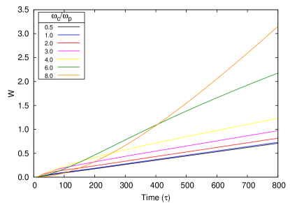
Figure 7: Temporal evolution of the total energy of the wakefield (Eq. (11) is integrated over space for each time step) for different values of the external magnetic fields by numerically solving the set of equations.

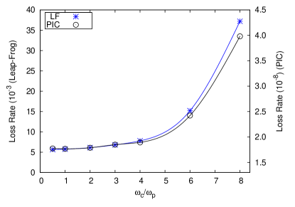
Figure 8: Energy loss rate as a function of ratio $\omega_{c}/\omega_{p}$ is presented for PIC as well as analytical results.

V Summary and Conclusion

In the present paper we have re-considered 1D wakefield generation in magnetized plasmas. Based on 1D PIC simulations we have deduced that previous results need to be modified in the regime of large magnetic fields. For moderate magnetic field strengths previous results are confirmed, and the wakefield consists of an extra-ordinary wave mode with a dominating frequency $\omega_{p}$ and wavenumber $\omega_{p}/c$. However, monitoring the dependence as a function of the frequency ratio $\omega_{c}/\omega_{p}$, we find that there is a gradual transition in the regime $2\lesssim\omega_{c}/\omega_{p}\lesssim 4$ where the wakefield spectrum of the extra-ordinary mode becomes broadband, and the loss rate of the high-frequency driver is enhanced..

Although we have deduced that wakefield generation is governed by Eqs. (8)- (10), we have not so far discussed why the assumption of a slow evolution in the co-moving frame must be abandoned for a large value of $\omega_{c}/\omega_{p}$. However, an explanation of this can be given in the form of a reductio ad absurdum reasoning. Let us assume that evolution of the extra-ordinary mode is indeed slow in the co-moving frame. In that case, there must be a dominant wavenumber of the wakefield corresponding to the property $v_{\phi wf}=v_{g}\approx c$, where $v_{g}$ is the group velocity of the high-frequency driving pulse and $v_{\phi wf}$ is the phase velocity of the wakefield. However, from the dispersion relation of the extra-ordinary mode we find that the group velocity for this wavenumber scales according to $v_{g}\rightarrow c$ for $\omega_{c}/\omega_{p}\rightarrow\infty$. This behavior is to a large extent reflected in Figs 2, 3 and 5, where the dominant mode follows the driver closely for the stronger values of the magnetic field. On the other hand provided the wakefield should follow the driver closely (as it must when $v_{g}\rightarrow c$) and then drop in amplitude suddenly, it cannot be well represented by a small spectrum surrounding a leading wave-number. Hence we must have broad-band wakefield spectrum for strong magnetic fields, in which case the assumption of a slow evolution of the wakefield will cease to be adequate.

To some extent the break-down of the slow evolution of the wakefield is related to the initial conditions. After long interaction times the system may gradually set up a wakefield with a dominating wave number, and at the same time the slow evolution regime can be approached. However, the stronger the magnetic field is, the longer time this will take. For a limited size of the plasma region and a strong magnetic field, in practice the slow evolution regime will never be reached. A practical consequence of this is that the loss rate of the high-frequency driver will be much enhanced, due to the excitation of the broad-band spectrum. Furthermore, the energy loss will be accompanied by a frequency decrease and  a de-acceleration of the driver Mironov1990 .

So far only the basic consequences of a strong magnetic field has been explored. A more complete study, e.g. involving the effects of varying the self-nonlinearity and the long-time evolution, is a project for further study.

- (1) T. Tajima and J. M. Dawson, Phys. Rev. Lett. 43, 267 (1979).
- (2) L. M. Gorbunov and V. I. Kirsanov, Zh. Eksp. Teor. Fiz. 93, 509 (1987) [Sov. Phys. JETP 66, 290 (1987)].
- (3) V. A. Balakirev, I. V. Karas and G. V. Sotnikov, Phys. Reports, 26, 889 (2000).
- (4) J. Faure, Y. Glinec, A. Pukhov, S. Kiselev, S. Gordienko, E. Lefebvre, J.-P. Rousseau, F. Burgy, and V. Malka, Nature 431, 541 (2004).
- (5) V. Malka, J. Faure, Y. A. Gauduel, E. Lefebvre, A. Rousse, and K. T. Phuoc, Nature Phys. 4, 447 (2008).
- (6) S. F. Martins, R. A. Fonseca, W. Lu, W. B. Mori, and L. O. Silva, Nature Phys. 6, 311 (2010).
- (7) V. A. Mironov, A. M. Sergeev, E. V. Vanin, G. Brodin, and J. Lundberg, Phys. Rev. A 46, R6178 (1992).
- (8) P. Chen, T. Tajima and Y. Takahashi, Phys. Rev. Lett. 89, 161101 (2002).
- (9) P.K. Shukla, G. Brodin, M. Marklund and L. Stenflo, Phys. Lett. A, 373, 3165 (2009).
- (10) N. Wadhwani, P. Kumar, and P. Jha, Phys. Plasmas, 9, 263 (2002).
- (11) P. K. Shukla, Phys. Plasmas 6, 1363 (1999).
- (12) G. Brodin and J. Lundberg, Phys. Rev. E 57, 7041 (1998).
- (13) J. Yoshii, C. H. Lai, T. Katsouleas, C. Joshi and W. B. Mori, Phys. Rev. Lett., 79, 4194 (1997).
- (14) H. Parchamy, N. Yugami, T. Muraki, H. Noda, Y. Nishida, Jap. J. Appl. Phys., 44, L196 (2005).
- (15) R. Lichters, R. E. W. Pfund, and J. Meyer-Ter-Vehn, Report MPQ 225, (1997).(http://www.lichters.net/download.html)
- (16) The coordinate system used in LPIC++ is different. Here we have changed the labels to make it consistent with rest of the paper.