Improving PSF calibration in confocal microscopic imaging—estimating and exploiting bilateral symmetry

Abstract

A method for estimating the axis of reflectional symmetry of an image $f(x,y)$ on the unit disc $D=\{(x,y)\dvtx x^{2}+y^{2}\leq 1\}$ is proposed, given that noisy data of $f(x,y)$ are observed on a discrete grid of edge width $\Delta$. Our estimation procedure is based on minimizing over $\beta\in[0,\pi)$ the $L_{2}$ distance between empirical versions of $f$ and $\tau_{\beta}f$, the image of $f$ after reflection at the axis along $(\cos\beta,\sin\beta)$. Here, $f$ and $\tau_{\beta}f$ are estimated using truncated radial series of the Zernike type. The inherent symmetry properties of the Zernike functions result in a particularly simple estimation procedure for $\beta$. It is shown that the estimate $\hat{\beta}$ converges at the parametric rate $\Delta^{-1}$ for images $f$ of bounded variation. Further, we establish asymptotic normality of $\hat{\beta}$ if $f$ is Lipschitz continuous. The method is applied to calibrating the point spread function (PSF) for the deconvolution of images from confocal microscopy. For various reasons the PSF characterizing the problem may not be rotationally invariant but rather only reflection symmetric with respect to two orthogonal axes. For an image of a bead acquired by a confocal laser scanning microscope (Leica TCS), these axes are estimated and corresponding confidence intervals are constructed. They turn out to be close to the coordinate axes of the imaging device. As cause for deviation from rotational invariance, this indicates some slight misalignment of the optical system or anisotropy of the immersion medium rather than some irregular shape of the bead. In an extensive simulation study, we show that using a symmetrized version of the observed PSF significantly improves the subsequent reconstruction process of the target image.

, and t1Supported by the BMBF project INVERS and of the DFG SFB 475 and SFB 823. t2Supported by the DFG Grant HO 3260/3-1, the Claussen–Simon–Stiftung and the Landesstiftung Baden-Württemberg, “Juniorprofessorenprogramm.”

1 Introduction

The fundamental concept of symmetry of physical and biological objects has been thoroughly studied for a long time; cf., e.g., Conway, Burgiel and Goodman-Strauss (2008). In particular, symmetry plays an important role in image analysis and understanding and finds direct applications in object recognition, robotics, image animation and image compression; see Liu, Collins and Tsin (2004) for an overview of the subject of symmetry and related issues. The problem of detecting and measuring object symmetries has been tackled in the image processing and pattern analysis literature since the original works of Atallah (1985) and Friedberg (1986). For a comprehensive review of the literature see Liu, Collins and Tsin (2004) and Bissantz, Holzmann and Pawlak (2009). The role of symmetry in statistical inference is discussed in Viana (2008).

In this paper we propose an estimation procedure for the angle $\beta$ of the direction $(\cos\beta,\sin\beta)$ of the axis of reflectional symmetry of an image function $f$ from which discrete, noisy observations are available. The observations are taken on a grid of edge width $\Delta$, and the noise is modeled by stochastic errors. Existing methods either do not allow any noise or treat the effect of noise only empirically by simulations. Thus, to the best of our knowledge, our approach is the first which treats reflection symmetry estimation from a statistical point of view as a semiparametric estimation problem. Specifically, we show that for image functions $f$ of bounded variation the estimate $\hat{\beta}$ converges at a rate of $\Delta^{-1}$ and, further, for Lipschitz continuous $f$ we have asymptotic normality, which allows us to construct asymptotic confidence intervals for $\beta$.

The estimation procedure is based on minimizing over $\beta\in[0,\pi)$ the $L_{2}$ distance between empirical versions of $f$ and $\tau_{\beta}f$, the image of $f$ after reflection at the axis along $(\cos\beta,\sin\beta)$. Here, $f$ and $\tau_{\beta}f$ are estimated using truncated Zernike function expansions. The inherent symmetry properties of the Zernike functions yield a particularly simple estimation procedure for $\beta$. In the recent related papers [cf. Kim and Kim (1999) and Revaud, Lavoue and Baskurt (2008)], methods for estimating the rotation angle of an image invariant under a certain rotation, which also make use of the Zernike moments, have been proposed. However, the authors do not study any convergence aspects of the algorithms and confine their discussion to noise-free images.

Our methodology is applied to calibrating the point spread function (PSF) of a microscope in confocal microscopy. The PSF describes the blurring effect of the imaging process. Typical smoothing scales are of order $\approx$100 nm, which often is of similar order as the size of relevant structures in the target object. Hence, an exact knowledge of the PSF is essential to properly adjust (i.e., deconvolve) the observed image to recover the image of the target object.

A theoretical PSF may be computed from the optical properties of the microscope, it is rotationally invariant for a rotationally symmetric optical system. However, the true (empirical) PSF can deviate substantially from its theoretical shape, and is no longer rotationally invariant. Therefore, the PSF is estimated from images of point-like objects with known form. Since this process involves rather dim images, it is worthwhile to use additional information on the PSF to improve on its reconstruction.

Often, the empirical PSF is still expected to be reflection symmetric with respect to two (unknown) orthogonal axes, for example, if the detector plane is not in perfect agreement with the focal plane of the microscope; cf. Lehr, Sibarita and Chassery (1998) and Pankajakshan et al. (2008). Therefore, for an image of a bead acquired by a confocal laser scanning microscope (Leica TCS), in Bissantz, Holzmann and Pawlak (2009) we used hypotheses tests to assess rotational invariance as well as invariance under a rotation by $\pi$ (which is a consequence of invariance under reflections by two orthogonal axes) for the empirical PSF. While (for bead 2) rotational invariance was rejected, invariance under a rotation by $\pi$ (and hence reflection symmetry) was not rejected at the level of $5\%$.

Here, we estimate the axes of reflectional symmetry of the PSF and construct the corresponding confidence intervals. It turns out that the axes are very close to the coordinate axes of the imaging device. This indicates that the reason for the PSF to deviate from rotational invariance appears to be some (slight) misalignment of the optical system or anisotropy of the immersion medium used for object preparation rather than some random deviation from sphericity of the bead used to image the PSF.

Further, we propose to reduce the noise level in the PSF by a factor of 2 by averaging along the estimated axes. To investigate the practical merit of this strategy for recovery of a target image, we use a two-step simulation study. First, the PSF is estimated by four different methods, then the estimated PSFs are used for subsequent recovery of the target image, and the accuracy of these reconstructions are compared. For the PSF we use a simple nonparametric estimate of the PSF as well as a symmetrized version, together with correctly specified and slightly misspecified parametric models. It turns out that while the correctly specified parametric model performs best for recovering the target image, symmetrizing the nonparametric estimate greatly improves its performance, even beyond that of the slightly misspecified parametric model.

The paper is organized as follows. In Section 2 we introduce the theoretical Zernike moments and give their basic invariance properties. Further, we discuss how to estimate the moments from data generated by our observational model. In Section 3 we propose the estimation procedure for the angle $\beta$ of the direction $(\cos\beta,\sin\beta)$ of the axis of reflectional symmetry of the image function $f$, and discuss its statistical properties. This includes the issue of uniqueness as well as consistency, rate of convergence and asymptotic distribution of the estimate. Section 4 contains simulation studies concerning the finite sample properties of the estimator. In Section 5 we discuss reflection symmetry properties of an observed PSF of a confocal laser scanning microscope (Leica TCS). Further, in a simulation we show how incorporating reflection symmetry into a simple nonparametric estimate of the PSF significantly improves its properties in the image reconstruction process. Section 6 gives some concluding remarks, while technical proofs can be found in the supplementary material in Bissantz, Holzmann and Pawlak (2010).

2 The Zernike orthogonal basis and image reconstruction

Zernike functions, introduced as an orthogonal and rotationally invariant basis of polynomials on the disc in Zernike (1934), and their corresponding moments have been used extensively in image analysis and pattern recognition; see Bailey and Srinath (1996), Khotanzad and Hong (1990) and Mukundan and Ramakrishnan (1998). The Zernike basis has also been employed as an important tool for the statistical inference concerning the inverse problem of positron emission tomography [cf. Jones and Silverman (1989) and Johnstone and Silverman (1990)] and PSF estimation in fluorescence microscopy [cf. Dieterlen et al. (2004); Dieterlen et al. (2008)].

2.1 Zernike polynomials

In the following we identify two-dimensional space $\mathbb{R}^{2}$ with the complex plane $\mathbb{C}$ via $(x,y)\mapsto x+iy$, where $i$ is the imaginary unit. In particular, $e^{i\beta}$ is the unit vector $(\cos\beta,\sin\beta)$ at angle $\beta$ to the $x$ axis.

Now, the (complex) Zernike orthogonal polynomials are given by $V_{pq}(x,y)=R_{pq}(\rho)e^{iq\theta}$, $(x,y)\in D$, where $\rho=\sqrt{x^{2}+y^{2}}$, $\theta=\arctan(y/x)$ and $R_{pq}(\rho)$ is the radial Zernike polynomial given explicitly by

$$R_{pq}(\rho)=\sum_{l=0}^{(p-|q|)/2}\frac{(-1)^{l}(p-l)!\rho^{p-2l}}{l!((p+|q|)/2-l)!((p-|q|)/2-l)!}.$$

The indices $(p,q)$ have to satisfy $p\geq 0$, $|q|\leq p$, and $p-|q|$ has to be even. We will call such pairs $(p,q)$ admissible. The Zernike polynomials satisfy the following orthogonality relation over the unit disc $D$:

$$\int\!\!\!\int_{D}V_{pq}(x,y)V_{p^{\prime}q^{\prime}}^{*}(x,y)\,dx\,dy=\pi/(p+1)\delta_{pp^{\prime}}\delta_{qq^{\prime}},$$

where ^∗ denotes complex conjugation and $\delta_{pp^{\prime}}$ is the Kronecker delta. This implies that

$$\|V_{pq}\|^{2}=\pi/(p+1)=n_{p},$$ (1)

where $\|\cdot\|$ is the norm on $L_{2}(D)$. In Bhatia and Wolf (1954), the Zernike polynomials are characterized by a certain uniqueness property, among others, invariant polynomials defined on $D$.

2.2 Function approximation

Since the family $\{V_{pq}(x,y)\}$ for admissible $(p,q)$ forms a complete and orthogonal system in $L_{2}(D)$, we can expand a function $f\in L_{2}(D)$ into a series of the Zernike polynomials, that is,

$$f(x,y)=\sum_{p=0}^{\infty}\sum_{q=-p}^{p}n_{p}^{-1}A_{pq}(f)V_{pq}(x,y),$$ (2)

where here and throughout the paper the summation is taken over admissible pairs $(p,q)$. Thus, the Fourier coefficients $\{A_{pq}(f)\}$ (often referred to as the Zernike moments) uniquely characterize the image function $f$. The norming factor $n_{p}^{-1}$ arises due to (1), and the Zernike moment $A_{pq}(f)$ is defined by

$$A_{pq}(f)=\int\!\!\!\int_{D}f(x,y)V_{pq}^{*}(x,y)\,dx\,dy.$$

Owing to Parseval’s formula, we have that for $f\in L_{2}(D)$

$$\|f\|^{2}=\sum_{p=0}^{\infty}\sum_{q=-p}^{p}n_{p}^{-1}|A_{pq}(f)|^{2}.$$ (3)

Let us introduce the notation $\tilde{f}(\rho,\theta)=f(\rho\cos\theta,\rho\sin\theta)$ for a function $f\in L_{2}(D)$. Then by using polar coordinates we obtain

$$A_{pq}(f) = 2\pi\int_{0}^{1}c_{q}(\rho,f)R_{pq}(\rho)\rho\,d\rho,$$

$$c_{q}(\rho,f) = \frac{1}{2\pi}\int_{0}^{2\pi}\tilde{f}(\rho,\theta)e^{-iq\theta}\,d\theta.$$

2.3 Image reconstruction

We assume that the data are observed on a symmetric square grid of edge width $\Delta$, that is, $x_{i}-x_{i-1}=y_{i}-y_{i-1}=\Delta$ and $x_{i}=-x_{m-i+1}$, $y_{i}=-y_{m-i+1}$, so that $(x_{i},y_{j})$ is the center of the pixel $\Pi_{ij}=[x_{i}-\frac{\Delta}{2},x_{i}+\frac{\Delta}{2}]\times[y_{j}-\frac{\Delta}{2},y_{j}+\frac{\Delta}{2}]$. Note that $m$ corresponds to $2/\Delta$. For $f\in L_{2}(D)$ we shall assume the following observational model:

$$Z_{i,j}=f(x_{i},y_{j})+\epsilon_{i,j},\qquad(x_{i},y_{j})\in D,1\leq i,j\leq m,$$ (5)

where the noise process $\{\epsilon_{i,j}\}$ is an i.i.d. random sequence with zero mean, finite variance $E\epsilon_{i,j}^{2}=\sigma^{2}$ and finite fourth moment, so that $Z_{i,j}$ is the datum associated with pixel $\Pi_{ij}$. Note that along the boundary of the disc, some lattice squares are included (if their center is in $D$) and some are excluded. When reconstructing $f$, this gives rise to an additional error, called geometric error in Pawlak and Liao (2002). This error can be quantified by using the celebrated problem in analytic number theory referred to as lattice points of the circle. In applications, the datum $Z_{i,j}$ might also correspond to the average of $f$ over the pixel $\Pi_{ij}$ rather than its value at the center, in such cases we assume negligible variation of $f$ over $\Pi_{ij}$.

In the following we need to work with a discretized version of the Zernike moments. Consider weights $w_{pq}(x_{i},y_{j})$ of the form

$$\quad w_{pq}(x_{i},y_{j})=\int\!\!\!\int_{\Pi_{ij}}V_{pq}^{*}(x,y)\,dx\,dy\quad\mbox{or}\quad w_{pq}(x_{i},y_{j})=\Delta^{2}V_{pq}^{*}(x_{i},y_{j}).$$ (6)

Using either version in (6), we estimate the Zernike moment $A_{pq}(f)$ by

$$\hat{A}_{pq}=\sum_{(x_{i},y_{j})\in D}w_{pq}(x_{i},y_{j})Z_{i,j}.$$ (7)

For efficient methods for computing the Zernike moments $\hat{A}_{pq}$, see, for example, Amayeh et al. (2005). Instead of the uniform weights, one could also use a more sophisticated quadrature rule, particularly if sharp features of $f$ are expected.

3 Reflection estimation

First we investigate the effect that reflecting an image function $f$ has on its Zernike moments. Suppose that $f$ is reflected at a line along the direction $e^{i\beta}$, $\beta\in[0,\pi)$, and denote the reflected function by $\tau_{\beta}f$. Then one easily shows that $\widetilde{(\tau_{\beta}f)}(\rho,\theta)=\tilde{f}(\rho,2\beta-\theta)$ and, consequently, using (2.2),

$$A_{pq}(\tau_{\beta}f)=e^{-2iq\beta}A_{p,-q}(f).$$ (8)

Consider the following assumption.

Assumption 1.

Suppose that $f\in L_{2}(D)$ is invariant under some unique reflection $\tau_{\beta^{*}}$.

Indeed, the composition of two reflections along lines $e^{i\alpha_{1}}$ and $e^{i\alpha_{2}}$ is a rotation with angle $2(\alpha_{2}-\alpha_{1})$. Thus, $f$ is invariant under a unique reflection if and only if $f$ is invariant under some reflection and if $f$ is not invariant under any rotation.

3.1 Contrast functions

Our method for estimating $\beta^{*}$ is based on the expansion (3) and the invariance property of Zernike moments expressed by the formula in (8). We set

$$M(\beta,f)=\|f-\tau_{\beta}f\|^{2}=\sum_{p=0}^{\infty}n_{p}^{-1}\sum_{q=-p}^{p}|A_{pq}(f)-e^{-2iq\beta}A_{p,-q}(f)|^{2}.$$ (9)

Evidently, under Assumption 1 the angle $\beta^{*}$ is the unique zero of the function $M(\beta,f)$. Writing $A_{pq}(f)=|A_{pq}(f)|e^{ir_{pq}(f)}$ and noting that $A_{pq}(f)=A_{p,-q}(f)^{*}$, we calculate

$$M(\beta,f)=\sum_{p=0}^{\infty}n_{p}^{-1}\sum_{q=0}^{p}4|A_{pq}(f)|^{2}\bigl{(}1-\cos\bigl{(}2r_{pq}(f)+2q\beta\bigr{)}\bigr{)},$$ (10)

where the sums are taken over admissible pairs $(p,q)$. Therefore, $\beta^{*}$ is also uniquely characterized by the condition $\cos(2r_{pq}(f)+2q\beta^{*})=1$ or by requiring

$$r_{pq}(f)\in q\beta^{*}+\pi\mathbb{Z}$$ (11)

for all $p,q$ with $A_{pq}(f)\not=0$.

Thus, a natural way to estimate $\beta^{*}$ is to first estimate a truncated version of the series defining $M(\beta,f)$, and then define an estimate of $\beta^{*}$ as the minimizer of this estimated contrast function. We first show that suitably truncated versions of $M(\beta,f)$ still uniquely determine $\beta^{*}$. For a fixed $N$ set

$$M_{N}(\beta,f)=\sum_{p=0}^{N}n_{p}^{-1}\sum_{q=-p}^{p}|A_{pq}(f)-e^{-2iq\beta}A_{p,-q}(f)|^{2}.$$

This is the truncated counterpart of the series in (9). Evidently, $M_{N}(\beta^{*},f)=0$ for all $N$ under Assumption 1. We shall call $M(\beta,f)$ and $M_{N}(\beta,f)$ as well as their empirical version below contrast functions.

Theorem 1.

Suppose that $f$ satisfies Assumption 1. Then for sufficiently large $N=N(f)$, $\beta^{*}$ is the unique zero of the truncated contrast functions $M_{N}(\beta,f)$.

The proof of Theorem 1, given in the supplementary material in Bissantz, Holzmann and Pawlak (2010), reveals that in order to uniquely determine the direction of the reflection axis $e^{i\beta^{*}}$ as the zero of the function $M_{N}(\beta,f)$ one has to choose $N$ so large such that the sum defining $M_{N}(\beta,f)$ contains nonzero $A_{pq}$’s for which the greatest common divisor (gcd) of the $q$’s is $1$. Thus, we can choose $N$ as the smallest value such that $A_{p_{1}q_{1}}(f)\neq 0,$ $\ldots,A_{p_{r}q_{r}}(f)\neq 0,$ for $p_{i}\leq N,i=1,\ldots,r$, with $\operatorname{gcd}(q_{1},\ldots,q_{r})=1.$

In practice, $M_{N}(\beta,f)$ and hence an appropriate value for $N$ still has to be estimated. One could test sufficiently many moments to be nonzero, however, we prefer to choose $N$ for appropriate estimation of $f$ in the resulting truncated Zernike series estimate; see Section 5. Apart from its theoretical value, Theorem 1 implies that even in dim images occurring, for example, in PSF estimation in Section 5, where only few Zernike moments may be properly estimated, it is still possible to identify and estimate the symmetry axis.

3.2 Estimation

For estimation purposes, we first estimate the contrast functions $M_{N}(\beta,f)$ by

$$\hat{M}_{N}(\beta)=\sum_{p=0}^{N}n_{p}^{-1}\sum_{q=-p}^{p}|\hat{A}_{pq}-e^{-2iq\beta}\hat{A}_{p,-q}|^{2},$$

where we write $\hat{A}_{pq}=|\hat{A}_{pq}|e^{i\hat{r}_{pq}}$. Then we define the estimator of $\beta^{*}$ as

$$\hat{\beta}_{\Delta,N}=\operatorname{arg}\min_{\beta\in[0,\pi)}\hat{M}_{N}(\beta).$$

The estimate $\hat{\beta}_{\Delta,N}$ depends on the grid size $\Delta$ and, more importantly, on the truncation parameter $N$. Note that although $M_{N}(\beta^{*})=0$, $\hat{M}_{N}(\hat{\beta}_{\Delta,N})$ will be positive a.s. due to noise.

Remark 1.

The estimated contrast function $\hat{M}_{N}(\beta)$ is simply the squared $L_{2}$ distance between the Zernike estimate given in polar coordinates by

$$\widetilde{{\hat{f}}}(\rho,\theta)=\sum_{(p,q)}^{N}n_{p}^{-1}\hat{A}_{p,q}\tilde{V}_{p,q}(\rho,\theta)$$

and its reflected version $\tau_{\beta}\hat{f}$. Note that this is achieved by a special property of the Zernike polynomials, namely, the set of Zernike polynomials used in the estimate $\hat{f}$ remains invariant under reflection. As suggested by a referee, an estimate similar to $\hat{\beta}_{\Delta,N}$ would be obtained by estimating the coefficients $A_{p,q}$ in

$$\tilde{f}(\rho,\theta)-\tau_{\beta}\tilde{f}(\rho,\theta)=\sum_{(p,q)}^{N}n_{p}^{-1}(A_{p,q}-A_{p,-q}e^{-2\beta iq})\tilde{V}_{p,q}(\rho,\theta)$$ (12)

by least squares for each fixed $\beta$, and then choosing the $\beta$ with minimal RSS. While our approach is somewhat simpler since we estimate the $A_{p,q}$ before imposing symmetry (and thus independently of $\beta$), this approach could potentially be placed into a likelihood or Bayesian framework as in Pankajakshan et al. (2008).

The next result states uniform convergence in probability of the estimated contrast function $\hat{M}_{N}(\beta)$ to $M_{N}(\beta)$. This is also used in order to obtain the consistency of $\hat{\beta}_{\Delta,N}$ for $\beta^{*}$.

Theorem 2.

For each fixed $N$, as $\Delta\to 0$,

$$\sup_{\beta\in[0,\pi)}|\hat{M}_{N}(\beta)-M_{N}(\beta,f)|\to 0\qquad(P),$$ (13)

where $(P)$ denotes convergence in probability.

Note that in Theorem 2, $f$ need not be reflection invariant. The next theorem gives the consistency of $\hat{\beta}_{\Delta,N}$ as $\Delta\to 0$ as well as its parametric $\Delta$-rate of convergence. In all the results that follow we choose the truncation parameter $N$ according to the prescription established in Theorem 1, that is, we require that $N$ should be selected in such a way that $\beta^{*}$ is the unique minimizer of $M_{N}(\beta,f).$ We will refer to such a value of $N$ as “sufficiently large.”

Theorem 3.

Suppose that $f\in L_{2}(D)$ is a function of bounded variation and satisfies Assumption 1. Then for sufficiently large (but fixed) $N=N(f)$, we have that, as $\Delta\to 0$,

$$|\hat{\beta}_{\Delta,N}-\beta^{*}|=O_{P}(\Delta).$$ (14)

Next we establish asymptotic normality for the estimate $\hat{\beta}_{\Delta,N}$. In order for the bias term of the estimated Zernike coefficient to be negligible, we require that the image function $f$ is Lipschitz continuous.

Theorem 4.

Suppose that $f$ is Lipschitz continuous and satisfies Assumption 1. Then for sufficiently large (but fixed) $N=N(f)$, we have that, as $\Delta\to 0$,

$$\Delta^{-1}(\hat{\beta}_{\Delta,N}-\beta^{*})\stackrel{{\scriptstyle\mathcal{L}}}{{\to}}N\biggl{(}0,\frac{8\sigma^{2}}{M_{N}^{\prime\prime}(\beta^{*},f)}\biggr{)},$$ (15)

where

$$M_{N}^{\prime\prime}(\beta^{*},f)=\sum_{p=0}^{N}n_{p}^{-1}\sum_{q=0}^{p}16|A_{pq}(f)|^{2}q^{2}.$$ (16)

Theorem 4 can be used to construct an asymptotic confidence interval for $\beta^{*}$. To this end, we need an estimate of the asymptotic variance in the normal limit (15). We may estimate $M_{N}^{\prime\prime}(\beta^{*},f)$ directly by using (16) simply by replacing $A_{pq}(f)$ by $\hat{A}_{pq}$. However, this may result in underestimation of the asymptotic variance, and therefore plugging $\hat{\beta}_{\Delta,N}$ into the second derivative of $\hat{M}_{N}(\beta$),

$$\hat{M}_{N}^{\prime\prime}(\beta)=\sum_{p=0}^{N}n_{p}^{-1}\sum_{q=0}^{p}16|\hat{A}_{pq}|^{2}q^{2}\cos(2\hat{r}_{pq}+2q\beta),$$

should generally be preferred. Call either estimate $\hat{M}_{N}^{\prime\prime}$. Further, we need to estimate the error variance $\sigma^{2}$. To this end, one could use the residuals from the fitted truncated Zernike series. We prefer to use a difference estimate of the form

$$\hat{\sigma}^{2}=\frac{1}{C(\Delta)}\sum_{(x_{i},y_{j})\in D}\frac{1}{4}\bigl{(}(Z_{i,j}-Z_{i+1,j})^{2}+(Z_{i,j}-Z_{i,j+1})^{2}\bigr{)},$$ (17)

which does not rely on the same underlying regression estimate. Here the sum is taken over all $(x_{i},y_{j})\in D$ where $(x_{i+1},y_{j})\in D$ and $(x_{i},y_{j+1})\in D$, and $C(\Delta)$ is the number of terms in this restricted sum. One can show that if $f$ is Lipschitz continuous, then $\hat{\sigma}^{2}-\sigma^{2}=O_{P}(\Delta)$. For detailed information on difference-based estimators in higher dimensions see Munk et al. (2005).

Using these estimates, we obtain the following confidence interval with nominal level $\alpha$ for $\beta^{*}$:

$$\biggl{[}\hat{\beta}_{\Delta,N}-u_{1-\alpha}\cdot\frac{2\sqrt{2}\hat{\sigma}\Delta}{(\hat{M}_{N}^{\prime\prime})^{1/2}},\hat{\beta}_{\Delta,N}+u_{1-\alpha}\cdot\frac{2\sqrt{2}\hat{\sigma}\Delta}{(\hat{M}_{N}^{\prime\prime})^{1/2}}\biggr{]},$$ (18)

where $u_{1-\alpha}$ is the $1-\alpha$-quantile of the standard normal distribution.

Remark 2.

If in Theorem 4 we only assume that $f\in L_{2}(D)$ is a function of bounded variation, then the bias is also of order $\Delta$, and we get an asymptotic offset (i.e., a limiting normal law with nonzero mean) in (15).

Remark 3.

If the image $f$ is not reflection invariant, the estimator $\hat{\beta}_{\Delta,N}$ may still converge to a certain parameter value $\beta^{\diamond}$, which is determined by minimizing the $L_{2}$-distance $\|f-\tau_{\beta}f\|^{2}$. Then $(f+\tau_{\beta^{\diamond}}f)/2$ is the best reflection-symmetric approximation (in the $L_{2}$ sense) to the original image $f$. However, since $\beta^{\diamond}$ is no longer a zero of the contrast function $M(\beta,f)$, Theorem 1 does not hold, and in order to achieve consistent estimation theoretically, one requires that $N\to\infty$.

Remark 4.

Suppose that $f$ is reflection invariant but is also invariant under some discrete rotation group. Then there will be a minimal angle $\alpha=2\pi/d$ for some $d\in\mathbb{N}$, under rotation of which $f$ is invariant. If we use the estimator $\hat{\beta}_{\Delta,N}$ in such a situation, then a unique reflection axis will be between $0$ and $\alpha$, and one should use the minimizer of $\hat{M}_{N}(\beta)$ in the interval $[0,\alpha)$ rather than in $[0,\pi)$.

4 Finite sample performance

4.1 Target functions and the shape of their contrast functions

In this section we discuss the results of a simulation study of the proposed estimation method for the angle $\beta$ of reflectional symmetry. We performed simulations with three target functions, which are given in polar coordinates by

$$f_{1}(\rho,\theta) = c_{1}\cdot x\cdot(1-\rho)\cdot\bigl{(}\sin\bigl{(}y+\sqrt{x^{2}+y^{4}}\bigr{)}+\sin\bigl{(}-y+\sqrt{x^{2}+y^{4}}\bigr{)}\bigr{)},$$

$$f_{2}(\rho,\theta) = c_{2}\cdot\rho\cdot(1-\rho)\cdot\bigl{(}e^{\cos(\theta)/0.02}+e^{\cos(\theta+0.6)/0.02}$$

$$\hskip 51.0pt\hskip 22.0pt{}+e^{\cos(\theta-0.3+\pi)/0.02}+e^{\cos(\theta+0.9+\pi)/0.02}\bigr{)},$$

$$f_{3}(\rho,\theta) = c_{3}\cdot\rho\cdot(1-\rho)\cdot\bigl{(}e^{\cos(\theta)/0.2}+e^{\cos(\theta+0.9)/0.2}+0.6\cdot e^{\cos(\theta-1.7)/0.2}\bigr{)},$$

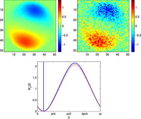
Figure 1: Reflection symmetric function $f_{1}$ without noise, with Gaussian noise, and $M_{7}(\beta)$ (full curve) and $\hat{M}_{7}(\beta)$ (dashed curve). Parameters are $n=25$ and signal-to-noise-ratio${}=5$. The vertical line indicates the direction of reflection symmetry in the true image.

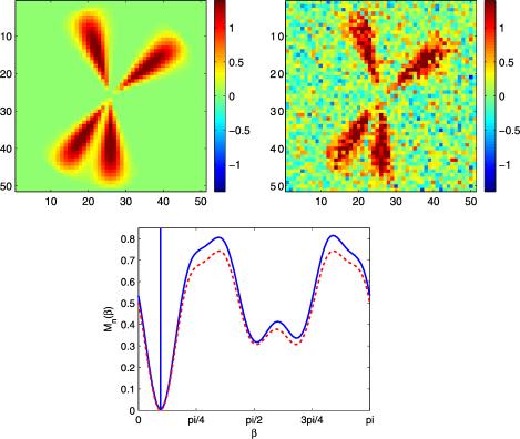
Figure 2: Reflection symmetric function $f_{2}$ without noise, with Gaussian noise, and $M_{7}(\beta)$ (full curve) and $\hat{M}_{7}(\beta)$ (dashed curve). Parameters are $n=25$ and signal-to-noise-ratio${}=5$. The vertical line indicates the direction of reflection symmetry in the true image.

where $x=\rho\cos(\theta)$, $y=\rho\sin(\theta)$, and $c_{1},c_{2},c_{3}$ are normalization constants such that the squared functions all integrate to one on the unit disc. Figures 1–3 show the target functions without noise and with Gaussian noise, where the signal-to-noise ratio, defined as the ratio between the peak values of the respective target function $f_{1},f_{2},f_{3}$ and the standard deviation of the noise $\sigma$, is $5$. Figure 4 again shows $f_{1}$ but with a signal-to-noise ratio of $16.7$. Note that the functions $f_{1}$ and $f_{2}$ are reflection symmetric, whereas $f_{3}$ is not. Moreover, in all cases we have used regularization parameters $N$ chosen according to the selection rule described in Bissantz, Holzmann and Pawlak (2009) (a stochastic analogue of the numerical discrepancy principle for parameter selection in inverse problems). The fact that $f_{1}$ and $f_{2}$, in contrast to $f_{3}$, are reflection symmetric is clearly expressed in the shape of the associated contrast functions. Indeed, $\hat{M}_{7}(\beta)$ is far above zero for $f_{3}$, in contrast to the case of $f_{1}$ and $f_{2}$, where $\hat{M}_{7}(\beta)$ reaches a minimum close to zero for noisy data. However, we note that even for $f_{3}$ there still exists a well-defined minimum of the contrast function $\hat{M}_{7}(\beta)$. The right panel in Figure 3 shows a reflection symmetric version of $f_{3}$, which has been generated by adding a version of $f_{3}$ mirrored w.r.t. the axis given by the direction of the minimum of $\hat{M}_{7}(\beta)$.

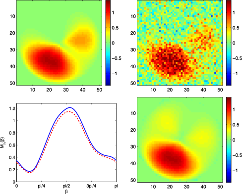
Figure 3: The function $f_{3}$ (which is not reflection symmetric) without noise, with Gaussian noise, and $M_{7}(\beta)$ (full curve), $\hat{M}_{7}(\beta)$ (dashed curve) and a symmetrized version of $f_{3}$. Parameters are $n=25$ and signal-to-noise-ratio${}=5$.

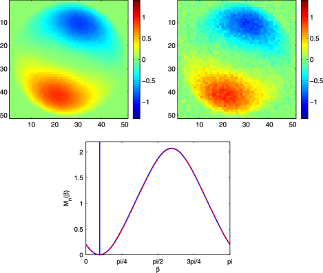
Figure 4: The reflection symmetric function $f_{1}$ without noise, with Gaussian noise, and $M_{7}(\beta)$ (full curve) and $\hat{M}_{7}(\beta)$ (dashed curve). Parameters are $n=25$ and signal-to-noise-ratio${}=16.7$. The vertical line indicates the direction of reflection symmetry in the true image.

4.2 Simulated distributions of estimated directions $\hat{\beta}$

In the second part we have simulated the distribution of $\hat{\beta}$, determined as the minimum of $\hat{M}_{N}(\beta)$, for a range of values for the parameters $n$ and the signal-to-noise ratio $s/n$. Figures 5 and 6 show density plots of the simulated distributions together with normal limits. For the reflection symmetric functions $f_{1}$ and $f_{2}$ we compare the simulated distributions to their asymptotic counterparts according to (15). Even for images of moderate size such as the unit circle in the square image with edge length $(2m+1)=51$ pixels, the simulated distributions are already close to their asymptotic limit.

Figure 5: Simulated (solid curve) and asymptotic (dashed curve) distributions of $\hat{\beta}_{\Delta,N}$ for $f_{1}$. The variance of the asymptotic distributions is given as $\frac{8\sigma^{2}\Delta^{2}}{M^{\prime\prime}_{N}(\beta^{\ast})}$ (cf. Theorem 3). The parameter $N$ was chosen as $7,8,12$ (first row, left to right) and $8,12,12$ (second row, left to right).

Figure 6: Simulated (solid curve) and asymptotic (dashed curve) distributions of $\hat{\beta}_{\Delta,N}$ for $f_{2}$ (left panels) and $f_{3}$ (right panels). The variance of the asymptotic distributions is given as $\frac{8\sigma^{2}\Delta^{2}}{M^{\prime\prime}_{N}(\beta^{\ast})}$ (cf. Theorem 3). The parameter $N$ was chosen as $7$, except for the lower left where it was chosen as $8$.

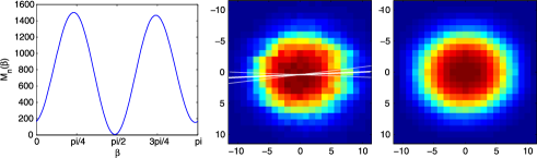
Figure 7: Contrast function of image bead (left), image bead with superposed estimated reflection axis and the associated asymptotic confidence interval with nominal level $95\%$ (middle), and bead after averaging along two estimated axes of reflectional symmetry (right). Bead was acquired during two observation runs of HeLa cervix carcinoma cells with a Leica TCS laser scanning fluorescence microscope. Here, we used $N=4$.

5 Calibrating the PSF in confocal microscopy

5.1 Assessing reflectional symmetry of the PSF

In this section we use the contrast function to estimate the axes of reflection symmetry in an image of the point-spread function in confocal fluorescence microscopic imaging. Here one observes count data representing observed pixel-integrated image intensities on a two-dimensional (or three-dimensional) equidistant grid of pixels. We consider the two-dimensional case, where the observations are $Z_{i,j}=(K\gamma)(x_{i},y_{j})+\varepsilon_{ij}$, with

$$(K\gamma)(x,y)=k\ast\gamma(x,y)=\int_{\mathbb{R}^{2}}k(x-t_{1},y-t_{2})\gamma(t_{1},t_{2})\,dt_{1}\,dt_{2},$$ (19)

and where “$\ast$” represents the convolution of the “true” image $\gamma\in L^{2}$ with the so-called point-spread-function (PSF) $k\in L^{2}$ of the microscope. The standard model for the distribution of the photon count data $Z_{i,j}$ is that $Z_{i,j}$ is Poisson with the mean $(K\gamma)(x_{i},y_{j})$, all independent.

The PSF represents the image of a point-source observed by the microscope and describes the blurring effect of the imaging process. As discussed in the introduction, the PSF is typically estimated by observing a point-like object (called bead) of known form. Figure 7 (right) shows the image of a bead under a Leica TCS confocal laser scanning microscope. The (observed) empirical PSF is typically no longer rotationally invariant, but it often remains reflection symmetric under two (unknown) orthogonal axes, even if, for example, the detector plane was not in perfect agreement with the focal plane of the microscope; cf. Lehr, Sibarita and Chassery (1998) and Pankajakshan et al. (2008).

In Bissantz, Holzmann and Pawlak (2009) we applied tests both for rotational invariance and for invariance under a rotation by $\pi$ (which is an immediate consequence of reflection symmetry w.r.t. two orthogonal axes) to the observed PSF in the image bead (Figure 7). It turned out that rotational invariance could be rejected at a 5% level, but invariance under a rotation by $\pi$ was not rejected.

For a deeper investigation, we now apply our methodology to estimate the (orthogonal) axes of reflection symmetry. The data from fluorescence microscopic imaging in general is distributed (approximately) according to a Poisson distribution with expectation given by the respective image intensity. Hence, the noise is not homoscedastic as required by model (5). As suggested by a referee, we use the (variance stabilizing) Anscombe transform [Anscombe (1948)]. Note that reflection symmetry is preserved in this process. Further, following Remark 4, we restrict the range of $\beta$ to $[\pi/4,3\pi/4]$, which yields an estimated angle and associated $95\%$ confidence interval of $\hat{\beta}=1.54\pm 0.07$. The truncation parameter was selected as $N=4$ by the method described in Bissantz, Holzmann and Pawlak (2009). Using the untransformed data and ignoring heteroscedasticity yields quite similar results ($\hat{\beta}=1.53\pm 0.08$), thus, heteroscedasticity appears to be a minor problem in this context.

Figure 7 (left and middle) shows the contrast function (of the untransformed data with $N=4$) and the image with superposed estimated reflection axis ($\hat{\beta}\approx 1.53$). The optical axis appears to be rather close to the coordinate axis of the image. In particular, the coordinate axis is covered by the associated $95\%$-nominal level confidence interval for $\hat{\beta}$ [cf. (18)]. This indicates that the reason for a PSF which is not rotationally invariant appears to be some (slight) misalignment of the optical system or anisotropy of the immersion medium used for object preparation rather than some random deviation from sphericity of the bead used to image the PSF. In Figure 7 (right), we plot the PSF after averaging along two estimated axes of reflectional symmetry.

5.2 Performance of symmetrized PSF estimates for image reconstruction

In this section we discuss the results from an extensive simulation study in which we investigate the potential benefit of incorporating symmetry information into PSF estimates.

We shall compare the performance of several models for the PSF for subsequent image reconstruction in a two-step simulation procedure which mimics the observational process in confocal microscopy. In the first step, we generate an image of a point-like object and use it to estimate the PSF in the distinct model classes. In the second step, these estimated PSFs are employed to reconstruct (by deconvolution with the estimated PSFs) a target image, and the accuracy of the resulting reconstructions is compared.

Inference on the PSF as required in the first step has to be conducted from dim images, and hence requires low-dimensional modeling. A possible approach is to use a parametric model; however, this involves the risk of misspecification. As an alternative, one could seek nonparametric estimates for the PSF. Due to the dimness of the image, nonparametric smoothing algorithms would require a substantial amount of smoothing. Therefore, the essential local feature of the PSF, the steep central peak, would be reduced, and hence its optical transfer function would be distorted. Thus, as an actual estimate of the PSF for the reconstruction process, the Zernike series estimates or other smoothed estimates should not be used. However, we argue that even for a dim image the Zernike estimate with few Zernike moments can be used for recovering the global feature of reflectional symmetry. Averaging along the estimated axes then reduces the noise level in the PSF reconstruction, which improves the reconstruction in step 2.

Specifically, the true PSF in the first step in the simulations consists of a bivariate Gaussian density function with full width at half maximum [FWHM] of $250$ nm along the $y$-axis and $250/\sqrt{2}$ nm along the $x$-axis, and the bead used to estimate the PSF is assumed to be $50$ nm in diameter. Moreover, the (true) peak intensity in the image of the bead is $\approx$22, which yields a signal-to-noise ratio for the brightest pixels of $\approx$5.

We use four models in which we estimate the PSF from the available (Poisson-distributed) observations. First, we use two parametric models, one correctly specified (i.e., the intensities have the shape of a Gaussian density with unknown covariance matrix), the other slightly misspecified with intensity function proportional to $\exp(\mbox{--}1/2(q(x,y))^{0.95})$ where $q(x,y)=(x,y)\Sigma^{-1}(x,y)^{T}$. Both models are estimated by maximum likelihood. Further, we use two nonsmoothed nonparametric estimates. The first simply consists of the observed raw data, for the second we average the raw data along the two estimated axes of reflectional symmetry, thereby reducing the noise level by a factor 2.

In the second step we aim to recover the target image plotted in Figure 8 from Poisson-observations with intensities given in (19), that is, the convolution of the target image and the true PSF described above. The target image is of size 8.2 µm along the $x$ and $y$-directions and with $128\times 128$ pixels along each axis, that is, the resolution of a pixel is $\approx$64 nm. The signal-to-noise ratio of the brightest pixels is $\approx$20 (and correspondingly lower for most of the image). For the image reconstruction by deconvolution, the distinct estimated PSFs are employed in the same algorithm. We use the Expectation Maximization method [cf. Shepp and Vardi (1982)], also called the Richardson–Lucy algorithm [cf. Richardson (1972) and Lucy (1974)], which is one of the most commonly used algorithms for deconvolution problems with positivity constraint. For each estimate of the PSF we record the smallest $L_{1}$- and $L_{2}$-distances attained between any iterate of the Richardson–Lucy reconstruction based on the respective PSF and the true target image in Figure 8.

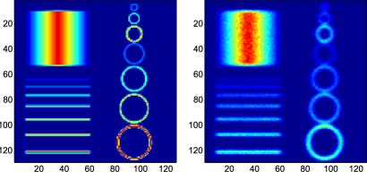
Figure 8: Test image used in the simulations of the benefit from using an estimated axis of symmetry for the PSF. Left: true image; right: convolved image with Gaussian noise.

Table 1: Mean optimal $L_{1}$- and $L_{2}$-distance achieved between reconstructed image and true image, based on three different estimates of the PSF

Distance	Parametric	Parametric	Nonparametric	Nonparametric
measure		(misspecified)	without symmetry	with symmetry
$L_{1}$ $(\times 10^{5})$	$1.3$	$1.9$	$2.0$	$1.7$
$L_{2}$ $(\times 10^{7})$	$0.6$	$1.6$	$1.5$	$1.2$

Table 1 shows the mean optimal $L_{1}$- and $L_{2}$-distances from $200$ simulations of the imaging process, that is, subsequent execution of steps 1 and 2. It turns out that while the correctly specified parametric model performs best for recovering the target image, symmetrizing the nonparametric estimate greatly improves its performance, even beyond that of the slightly misspecified parametric model.

6 Conclusions

Detection and estimation of symmetry are fundamental concepts in many areas of science and technology. In particular, the concept of symmetry plays an important role in image analysis and pattern recognition.

Symmetry is also relevant in many statistical models. An important and well-studied example is the symmetric location model $h(x-\theta),$ where $h(x)=h(-x)$ is an unknown symmetric density function and $\theta\in\mathbb{R}$ is the location parameter. Such models consisting of a Euclidean parameter as well as a nonparametric component are called semiparametric, and efficient, that is, asymptotically optimal estimation procedures in such problems are important and difficult issues in statistical inference [Bickel et al. (1993)].

In this paper we have discussed how to estimate the angle of the axis of reflectional symmetry of an image function, and studied its asymptotic properties. This problem is also of a semiparametric form, with the angle $\beta$ as the target parameter, and the image function (that is reflection symmetric with respect to a fixed axis, say, the $x$-axis) as nonparametric component. Although we showed that the parametric rate is achievable for estimating the parameter $\beta$, and also obtained an asymptotic normal law, we did not go into the problem of semiparametric efficiency and leave this issue for future research.

We have applied our method to calibrating the point-spread function (PSF) in confocal microscopy. In particular, we have shown how reflection symmetry (but no rotational invariance) may arise in the PSF. Further, we demonstrated that estimating the symmetry axes and symmetrizing the image of the PSF reduces the noise level in nonparametric estimates, and can lead to substantial improvement in the performance in subsequent image reconstruction algorithms.

Future research will be directed toward elucidating symmetry information and estimation in more complex microscopic setups, in particular, in 3D-fluorescence microscopy [e.g., 4PI-microscopy as in Bewersdorf, Schmidt and Hell (2006)].

References

- (1) Amayeh, G., Erol, A., Bebis, G. and Nicolescu, M. (2005). Accurate and efficient computation of high order Zernike moments. In Advances in Visual Computing 462–469. Springer, Berlin.
- (2) Anscombe, F. J. (1948). The transformation of Poisson, binomial and negative-binomial data. Biometrika 35 246–254. \MR0028556
- (3) Atallah, M. J. (1985). On symmetry detection. IEEE Trans. Comput. 34 663–666. \MR0800338
- (4) Bailey, R. R. and Srinath, M. (1996). Orthogonal moment feature for use with parametric and non-parametric classifiers. IEEE Trans. Pattern Anal. Mach. Intell. 18 389–396.
- (5) Bewersdorf, J., Schmidt, R. and Hell, S. W. (2006). Comparison of and 4Pi-microscopy. J. Microscopy 222 105–117. \MR2242148
- (6) Bickel, P. J., Klaassen, C. A. J., Ritov, Y. and Wellner, J. A. (1993). Efficient and Adaptive Estimation for Semiparametric Models. Johns Hopkins Univ. Press, Baltimore, MD. \MR1245941
- (7) Bissantz, N., Holzmann, H. and Pawlak, M. (2009). Testing for image symmetries—with application to confocal miscroscopy. IEEE Trans. Inform. Theory 55 1841–1855. \MR2582770
- (8) Bissantz, N., Holzmann, H. and Pawlak, M. (2010). Estimating bilateral symmetry: Technical details. Supplement to “Improving PSF calibration in confocal microscopic imaging—estimating and exploiting bilateral symmetry.” DOI: 10.1214/10-AOAS343SUPP.
- (9) Bhatia, A. B. and Wolf, E. (1954). On the circle polynomials of Zernike and related orthogonal sets. Proc. Cambridge Philos. Soc. 50 40–48. \MR0058021
- (10) Conway, J. H., Burgiel, H. and Goodman-Strauss, C. (2008). The Symmetry of Things. A. K. Peters, Wellesley, MA.
- (11) Dieterlen, A., Debailleul, M., De Meyer, A., Simon, B., Georges, V., Colicchio, B. and Haeberlé, O. (2008). Recent advances in 3-D fluorescence microscopy: Tomography as a source of information. In Eighth International Conference on Correlation Optics (M. Kujawinska and O. V. Angelsky, eds.). Proc. SPIE 7008 70080S–70080S-8. SPIE.
- (12) Dieterlen, A., Xu, C., Haeberle, O., Hueber, N., Malfara, R., Colicchio, B. and Jacquey, S. (2004). Identification and restoration in 3D fluorescence microscopy. In Sixth International Conference on Correlation Optics (O. V. Angelsky, ed.). Proc. SPIE 5477 105–113. SPIE.
- (13) Friedberg, S. A. (1986). Finding axes of skewed symmetry. Comput. Vision Graphics Image Process 32 138–155.
- (14) Johnstone, I. M. and Silverman, B. W. (1990). Speed of estimation in positron emission tomography and related inverse problems. Ann. Statist. 18 251–280. \MR1041393
- (15) Jones, M. C. and Silverman, B. W. (1989). An orthogonal series density estimation approach to reconstructing positron emission tomography images. J. Appl. Statist. 16 177–191.
- (16) Kim, W.-Y. and Kim, Y.-S. (1999). Robust rotation angle estimator. IEEE Trans. Pattern Anal. Mach. Intell. 21 768–773.
- (17) Khotanzad, A. and Hong, Y. H. (1990). Invariant image recognition by Zernike moments. IEEE Trans. Pattern Anal. Mach. Intell. 12 489–498.
- (18) Lehr, J., Sibarita, J.-B. and Chassery, J.-M. (1998). Image restoration in X-ray microscopy: PSF determination and biological applications. IEEE Trans. Image Processing 7 258–263.
- (19) Liu, Y., Collins, R. T. and Tsin, Y. (2004). A computational model for periodic pattern perception based on frieze and wallpaper groups. IEEE Trans. Pattern Anal. Mach. Intell. 26 354–371.
- (20) Lucy, L. B. (1974). An iterative technique for the rectification of observed distributions. Astron. J. 79 745–754.
- (21) Mukundan, R. and Ramakrishnan, K. (1998). Moment Functions in Image Analysis: Theory and Applications. World Scientific, River Edge, NJ. \MR1695522
- (22) Munk, A., Bissantz, N., Wagner, T. and Freitag, G. (2005). On difference-based variance estimation in nonparametric regression when the covariate is high dimensional. J. Roy Statist. Soc. B 67 19–41. \MR2136637
- (23) Pankajakshan, P., Zhang, B., Blanc-Féraud, L., Kam, Z., Olivo-Marin, J.-C. and Zerubia, J. (2008). Blind deconvolution for diffraction-limited fluorescence microscopy. IEEE International Symposium on Biomedical Imaging.
- (24) Pawlak, M. and Liao, S. X. (2002). On the recovery of a function on a circular domain. IEEE Trans. Inform. Theory 48 2736–2753. \MR1930340
- (25) Revaud, J., Lavoue, G. and Baskurt, A. (2008). Improving Zernike moments comparison for optimal similarity and rotation angle retrieval. IEEE Trans. Pattern Anal. Mach. Intell. 30 954–971.
- (26) Richardson, W. H. (1972). Bayesian-based iterative method of image restoration. J. Opt. Soc. Am. 62 55–59.
- (27) Shepp, I. A. and Vardi, Y. (1982). Maximum likelihood reconstruction for emission tomography. IEEE Trans. Med. Imaging 1 113–122.
- (28) Viana, M. A. G. (2008). Symmetry Studies: An Introduction to the Analysis of Structured Data in Applications. Cambridge Univ. Press, Cambridge. \MR2419845
- (29) Zernike, F. (1934). Beugungstheorie des Schneidenverfahrens und seiner verbesserten Form, der Phasenkontrastmethode. Physica 1 689–701.