Stellar weak decay rates in neutron-deficient medium-mass nuclei

Abstract

Weak decay rates under stellar density and temperature conditions holding at the rapid proton capture process are studied in neutron-deficient medium-mass waiting point nuclei extending from Ni up to Sn. Neighboring isotopes to these waiting point nuclei are also included in the analysis. The nuclear structure part of the problem is described within a deformed Skyrme Hartree-Fock + BCS + QRPA approach, which reproduces not only the beta-decay half-lives but also the available Gamow-Teller strength distributions, measured under terrestrial conditions. The various sensitivities of the decay rates to both density and temperature are discussed. In particular, we study the impact of contributions coming from thermally populated excited states in the parent nucleus, as well as the competition between beta decays and continuum electron captures.

I Introduction

An accurate understanding of most astrophysical processes requires necessarily information from nuclear physics, which provides the input to deal with network calculations and astrophysical simulations (see langanke03 ; apra and references therein). Obviously, nuclear physics uncertainties will finally affect the reliability of the description of those astrophysical processes. This is especially relevant in the case of explosive phenomena, which involve knowledge of the properties of exotic nuclei, not well explored yet. Thus, most of the astrophysical simulations of these violent events must be built on nuclear-model predictions of limited quality and accuracy. This is in particular the case of the X-ray bursts (XRBs) wallace ; thielemann ; schatz ; woosley , which are generated by a thermonuclear runaway in the hydrogen-rich environment of an accreting neutron star that is fed from a red giant binary companion close enough to allow for mass transfer.

Type I XRBs are typically characterized by a rapid increase in luminosity generating burst energies of $10^{39}-10^{40}$ ergs, which are typically a factor 100 larger than the steady luminosity. The luminosity suffers a sharp raise of about $1-10$ s followed by a gradual softening with time scales between 10 and 100 s. These bursts are recurrent with time scales ranging from hours to days. The properties of XRBs are particularly dependent on the accretion rate. Typical accretion rates for type I XRBs are about $10^{-8}-10^{-9}M_{\odot}$ yr^-1. Lower accretion rates lead to weaker flashes while larger accretion rates lead to stable burning on the surface of the neutron star.

The ignition of XRBs takes place when the temperature ($T$) and the density ($\rho$) in the accreted disk become high enough to allow a breakout from the hot CNO cycle. Peak conditions of $T=1-3$ GK and $\rho=10^{6}-10^{7}$ g cm^-3 are reached and eventually, this scenario allows the development of the nucleosynthesis rapid proton capture ($rp$) process schatz ; woosley ; wormer ; pruet , which is characterized by proton capture reaction rates that are orders of magnitude faster than any other competing process, in particular $\beta$-decay. It produces rapid nucleosynthesis on the proton-rich side of stability toward heavier proton-rich nuclei reaching nuclei with $A\gtrsim 100$, as it have been studied in Ref. schatz01 , where it was shown that the $rp$ process ends in a closed SnSbTe cycle. It also explains the energy and luminosity profiles observed in XRBs.

Nuclear reaction network calculations, which may involve as much as several thousand nuclear processes, are performed to follow the time evolution of the isotopic abundances, to determine the amount of energy released by nuclear reactions, and to find the reaction path for the $rp$ process wallace ; thielemann ; schatz ; woosley ; wormer ; pruet ; schatz01 ; ffn . In general, the reaction path follows a series of fast proton-capture reactions until the dripline is reached and further proton capture is inhibited by a strong reverse photodisintegration reaction. At this point, the process may only proceed through a beta decay or a less probable double proton capture. Then the reaction flow has to wait for a relatively slow $\beta$-decay and the respective nucleus is called a waiting point (WP). The short time scale of the $rp$ process (around 100 s) makes highly significant any mechanism that may affect the process in some seconds and the half-lives of the WP nuclei are of this order. Therefore, the half-lives of the WP nuclei along the reaction path determine the time scale of the nucleosynthesis process and the produced isotopic abundances. In this respect, the weak decay rates of neutron-deficient medium-mass nuclei under stellar conditions play a relevant role to understand the $rp$ process.

Although the products of the nucleosynthesis $rp$ process are not expected to be ejected from type I XRBs due to the strength of the neutron star gravitational field, there are other speculative sites for the occurrence of $rp$ processes. This is the case of core collapse supernovae that might supply suitable physical conditions for the $rp$ process provided neutrino-induced reactions are included in the nucleosynthesis calculations wanajo . These reactions have to be included to bypass the slow beta decays at the WP nuclei via capture reactions of neutrons, which are created from the antielectron neutrino absorption by free protons frohlich . Contrary to the XRBs, these scenarios will finally lead to the ejection of the nucleosynthetic products and thus contribute to the galactic chemical evolution.

Since the pioneering work of Fuller, Fowler and Newman ffn , where the general formalism to calculate weak-interaction rates in stellar environments as a function of density and temperature was introduced, improvements have been focused on the description of the nuclear structure aspect of the problem. Different approaches to describe the nuclear structure involved in the stellar weak decay rates can be found in the literature. They are basically divided into Shell Model langanke00 ; langanke01 or quasiparticle random phase approximation (QRPA) nabi ; paar09 ; sarri_plb categories. Certainly, the nuclear structure problem involved in the calculation of these rates must be treated in a reliable way. In particular, this implies that the nuclear models should be able to describe at least the experimental information available on the decay properties (Gamow-Teller strength distributions and $\beta$-decay half-lives) measured under terrestrial conditions. Although these decay properties may be different at the high $\rho$ and $T$ existing in $rp$ process scenarios, success in describing the decay properties in terrestrial conditions is a requirement for a reliable calculation of the weak decay rates in more general conditions. With this aim in mind, we study here the dependence of the decay rates on both $\rho$ and $T$ using a QRPA approach based on a selfconsistent deformed Hartree-Fock (HF) mean field. Deformation has to be taken into account because the reaction path in the $rp$ process crosses a region of highly deformed nuclei around $A=70-80$. This nuclear model has been tested successfully (see sarri_prc and references therein) and reproduces very reasonably the experimental information available on both bulk and decay properties of medium-mass nuclei. In this work we focus our attention to the even-even WP Ni, Zn, Ge, Se, Kr, Sr, Zr, Mo, Ru, Pd, Cd, and Sn isotopes, as well as to their closer even-even neighbors.

The paper is organized as follows. In Section II the weak decay rates are introduced as functions of density and temperature and their nuclear structure and phase space components are studied. Section III contains the results. First, we study the decay properties under terrestrial conditions, and secondly as functions of both densities and temperatures at the $rp$ process. Section IV contains the conclusions of this work.

II Weak decay rates

There are several distinctions between terrestrial and stellar decay rates caused by the effect of high $\rho$ and $T$. The main effect of $T$ is directly related to the thermal population of excited states in the decaying nucleus, accompanied by the corresponding depopulation of the ground states. The weak-decay rates of excited states can be significantly different from those of the ground state and a case by case consideration is needed. Another effect related to the high $\rho$ and $T$ comes from the fact that atoms in these scenarios are completely ionized and consequently electrons are no longer bound to the nuclei, but forming a degenerate plasma obeying a Fermi-Dirac distribution. This opens the possibility for continuum electron capture ($cEC$), in contrast to the orbital electron capture ($oEC$) produced by bound electrons in the atom under terrestrial conditions. These effects make weak interaction rates in the stellar interior sensitive functions of T and $\rho$, with $T=1.5$ GK and $\rho=10^{6}$ g cm^-3, as the most significant conditions for the $rp$ process schatz .

The decay rate of the parent nucleus is given by

$$\lambda=\sum_{i}\lambda_{i}\,\frac{2J_{i}+1}{G}e^{-E_{i}/(kT)}\,,$$ (1)

where $G=\sum_{i}\left(2J_{i}+1\right)e^{-E_{i}/(kT)}$ is the partition function, $J_{i}(E_{i})$ is the angular momentum (excitation energy) of the parent nucleus state $i$, and thermal equilibrium is assumed. In principle, the sum extends over all populated states in the parent nucleus up to the proton separation energy. However, since the range of temperatures for the $rp$ process peaks at $T=1.5$ GK ($kT\sim 300$ keV), only a few low-lying excited states are expected to contribute significantly in the decay. Specifically, we consider in this work all the collective low-lying excited states below 1 MeV ensdf . Two-quasiparticle excitations in even-even nuclei will appear at an excitation energy above 2 MeV, which is a typical energy to break a pair in these isotopes. Hence, they can be safely neglected at these temperatures. As an example, the maximum population appears for the lowest of these states ($E_{2^{+}}=261$ keV in ⁷⁶Sr), which at $T$=1.5 GK is $12\%$, while the ground state still contributes with $88\%$.

The decay rate for the parent state $i$ is given by

$$\lambda_{i}=\sum_{f}\lambda_{if}\,,$$ (2)

where the sum extends over all the states in the final nucleus reached in the decay process. The rate $\lambda_{if}$ from the initial state $i$ to the final state $f$ is given by

$$\lambda_{if}=\frac{\ln 2}{D}B_{if}\Phi_{if}(\rho,T)\,,$$ (3)

where $D=6146$ s. This expression is decomposed into a nuclear structure part $B_{if}$ that contains the transition probabilities for allowed Fermi (F) and Gamow-Teller (GT) transitions,

$$B_{if}=B_{if}(GT)+B_{if}(F)\,,$$ (4)

and a phase space factor $\Phi_{if}$, which is a sensitive function of $\rho$ and $T$. The theoretical description of both $B_{if}$ and $\Phi_{if}$ are explained in the next subsections.

II.1 Nuclear Structure

The nuclear structure part of the problem is described within the QRPA formalism. Various approaches have been developed in the past to describe the spin-isospin nuclear excitations in QRPA krum ; hamamoto ; moller ; hir ; homma ; borzov ; paar04 ; fracasso ; petro ; sarri_74 ; sarri_pp ; sarri_odd . In this subsection we show briefly the theoretical framework used in this paper to describe the nuclear part of the decay rates in the neutron-deficient nuclei considered in this work. More details of the formalism can be found in Refs. sarri_74 ; sarri_pp ; sarri_odd .

The method starts with a self-consistent deformed Hartree-Fock mean field formalism obtained with Skyrme interactions, including pairing correlations. The single-particle energies, wave functions, and occupation probabilities are generated from this mean field. In this work we have chosen the Skyrme force SLy4 sly4 as a representative of the Skyrme forces. This particular force includes some selected properties of unstable nuclei in the adjusting procedure of the parameters. It is one of the most successful Skyrme forces and has been extensively studied in the last years.

The solution of the HF equation is found by using the formalism developed in Ref. vautherin , assuming time reversal and axial symmetry. The single-particle wave functions are expanded in terms of the eigenstates of an axially symmetric harmonic oscillator in cylindrical coordinates, using twelve major shells. The method also includes pairing between like nucleons in BCS approximation with fixed gap parameters for protons and neutrons, which are determined phenomenologically from the odd-even mass differences involving the experimental binding energies audi .

The potential energy curves are analyzed as a function of the quadrupole deformation $\beta$,

$$\beta=\sqrt{\frac{\pi}{5}}\frac{Q_{0}}{A\langle r^{2}\rangle}\,,$$ (5)

written in terms of the mass quadrupole moment $Q_{0}$ and the mean square radius $\langle r^{2}\rangle$. For that purpose, constrained HF calculations are performed with a quadratic constraint constraint . The HF energy is minimized under the constraint of keeping fixed the nuclear deformation. Calculations for GT strengths are performed subsequently for the various equilibrium shapes of each nucleus, that is, for the solutions, in general deformed, for which minima are obtained in the energy curves. Since decays connecting different shapes are disfavored, similar shapes are assumed for the ground state of the parent nucleus and for all populated states in the daughter nucleus. The validity of this assumption was discussed for example in Refs. krum ; homma .

To describe GT transitions, a spin-isospin residual interaction is added to the mean field and treated in a deformed proton-neutron QRPA. This interaction contains two parts, a particle-hole ($ph$) and a particle-particle ($pp$). The interaction in the $ph$ channel is responsible for the position and structure of the GT resonance homma ; sarri_gese and it can be derived consistently from the same Skyrme interaction used to generate the mean field, through the second derivatives of the energy density functional with respect to the one-body densities. The $ph$ residual interaction is finally expressed in a separable form by averaging the resulting contact force over the nuclear volume sarri_74 . The $pp$ part is a neutron-proton pairing force in the $J^{\pi}=1^{+}$ coupling channel, which is also introduced as a separable force hir ; sarri_pp . The strength of the $pp$ residual interaction in this theoretical approach is not derived self-consistently from the SLy4 force used to obtain the mean field, but nevertheless it has been fixed in accordance to it. This strength is usually fitted to reproduce globally the experimental half-lives. Various attempts have been done in the past to fix this strength homma , arriving to expressions that depend on the model used to describe the mean field, Nilsson model in the above reference. In previous works sarri_pp ; sarri_gese ; sarri_pb ; sarri_wp ; sarri_pere we have studied the sensitivity of the GT strength distributions to the various ingredients contributing to the deformed QRPA-like calculations, namely to the nucleon-nucleon effective force, to pairing correlations, and to residual interactions. We found different sensitivities to them. In this work, all of these ingredients have been fixed to the most reasonable choices found previously sarri_prc and mentioned above. In particular we use the coupling strengths $\chi^{ph}_{GT}=0.15$ MeV and $\kappa^{pp}_{GT}=0.03$ MeV.

The proton-neutron QRPA phonon operator for GT excitations in even-even nuclei is written as

$$\Gamma_{\omega_{K}}^{+}=\sum_{\pi\nu}\left[X_{\pi\nu}^{\omega_{K}}\alpha_{\nu}^{+}\alpha_{\bar{\pi}}^{+}+Y_{\pi\nu}^{\omega_{K}}\alpha_{\bar{\nu}}\alpha_{\pi}\right]\,,$$ (6)

where $\alpha^{+}\left(\alpha\right)$ are quasiparticle creation (annihilation) operators, $\omega_{K}$ are the QRPA excitation energies, and $X_{\pi\nu}^{\omega_{K}},Y_{\pi\nu}^{\omega_{K}}$ the forward and backward amplitudes, respectively. For even-even nuclei the allowed GT transition amplitudes in the intrinsic frame connecting the QRPA ground state $\left|0\right\rangle\ \ \left(\Gamma_{\omega_{K}}\left|0\right\rangle=0\right)$ to one-phonon states $\left|\omega_{K}\right\rangle\ \ \left(\Gamma^{+}_{\omega_{K}}\left|0\right\rangle=\left|\omega_{K}\right\rangle\right)$, are given by

$$\left\langle\omega_{K}|\sigma_{K}t^{\pm}|0\right\rangle=\mp M^{\omega_{K}}_{\pm}\,,\quad K=0,1\,,$$ (7)

where

$$M_{-}^{\omega_{K}} = \sum_{\pi\nu}\left(q_{\pi\nu}X_{\pi\nu}^{\omega_{K}}+\tilde{q}_{\pi\nu}Y_{\pi\nu}^{\omega_{K}}\right),$$ (8)

$$M_{+}^{\omega_{K}} = \sum_{\pi\nu}\left(\tilde{q}_{\pi\nu}X_{\pi\nu}^{\omega_{K}}+q_{\pi\nu}Y_{\pi\nu}^{\omega_{K}}\right)\,,$$ (9)

with

$$\tilde{q}_{\pi\nu}=u_{\nu}v_{\pi}\Sigma_{K}^{\nu\pi},\ \ \ q_{\pi\nu}=v_{\nu}u_{\pi}\Sigma_{K}^{\nu\pi},$$ (10)

$v^{\prime}$s are occupation amplitudes ($u^{2}=1-v^{2}$) and $\Sigma_{K}^{\nu\pi}$ spin matrix elements connecting neutron and proton states with spin operators

$$\Sigma_{K}^{\nu\pi}=\left\langle\nu\left|\sigma_{K}\right|\pi\right\rangle\,.$$ (11)

The GT strength for a transition from an initial state $i$ to a final state $f$ is given by

$$B_{if}(GT^{\pm})=\frac{1}{2J_{i}+1}\left(\frac{g_{A}}{g_{V}}\right)_{\rm eff}^{2}\langle f||\sum_{j}^{A}\sigma_{j}t^{\pm}_{j}||i\rangle^{2}\,,$$ (12)

where $(g_{A}/g_{V})_{\rm eff}=0.74(g_{A}/g_{V})_{\rm bare}$ is an effective quenched value. For the transition $I_{i}K_{i}(0^{+}0)\rightarrow I_{f}K_{f}(1^{+}K)$ in the laboratory system, the energy distribution of the GT strength $B_{\omega}(GT^{\pm})$ is expressed in terms of the intrinsic amplitudes in Eq. (7) as

$$B_{\omega}(GT^{\pm}) = \left(\frac{g_{A}}{g_{V}}\right)_{\rm eff}^{2}\sum_{\omega_{K}}\left[\left\langle\omega_{K}\left|\sigma_{0}t^{\pm}\right|0\right\rangle^{2}\delta_{K,0}\right.$$ (13)

$$\left.+2\left\langle\omega_{K}\left|\sigma_{1}t^{\pm}\right|0\right\rangle^{2}\delta_{K,1}\right]\,.$$

To obtain this expression, the initial and final states in the laboratory frame have been expressed in terms of the intrinsic states using the Bohr-Mottelson factorization bm .

Concerning Fermi transitions, the Fermi operator is the isospin ladder operator $T_{\pm}$, which commutes with the nuclear part of the Hamiltonian excluding the small Coulomb component. Then, superallowed Fermi transitions ($0^{+}\rightarrow 0^{+}$) only occur between members of an isospin multiplet. The Fermi strength is narrowly concentrated in the isobaric analog state (IAS) of the ground state of the decaying nucleus. Thus, neglecting effects from isospin mixing one has

$$B_{if}(F^{\pm})=\frac{1}{2J_{i}+1}\langle f||\sum_{j}^{A}t^{\pm}_{j}||i\rangle^{2}=T(T+1)-T_{z_{i}}T_{z_{f}}\,,$$ (14)

where $T$ is the nuclear isospin and $T_{z}=(N-Z)/2$ its third component. The $B_{if}(F^{+})$ strength of our concern here reduces to $B(F^{+})=(Z-N)=2$ for the $(T,T_{z})=(1,-1)$ isotopes in the decay $(Z,N)\rightarrow(Z-1,N+1)$ with $Z=N+2$. For these transitions the excitation energy of the IAS in the daughter nucleus is given by pruet ; ffn

$$E_{IAS}=(ME)_{i}-(ME)_{f}+0.7824-\Delta E_{C}\,{\rm MeV},$$ (15)

where $ME$ is the atomic mass excess. The Coulomb displacement energy $\Delta E_{C}$ between pairs of isobaric analog levels is given by

$$\Delta E_{C}=1.4144{\bar{Z}}/A^{1/3}-0.9127{\rm MeV}\,,$$ (16)

where $\bar{Z}=(Z_{i}+Z_{f})/2$. This expression was obtained in Ref. antony from a fitting to data corresponding to levels with isospin $T=1$. In any case, Fermi transitions are only important for the $\beta^{+}$ decay of neutron-deficient light nuclei with $Z>N$ ($T_{z}<0$), where the IAS can be reached energetically. Thus, although they have been considered in the calculations of the terrestrial half-lives, only the dominant GT transitions are included in the stellar decay rates.

II.2 Phase Space Factors

The phase space factor contains two components, electron capture ($EC$) and $\beta^{+}$ decay

$$\Phi_{if}=\Phi^{EC}_{if}+\Phi^{\beta^{+}}_{if}\,.$$ (17)

In the case of $\beta^{+}/EC$ decay in the laboratory, $EC$ arises from orbital electrons in the atom and the phase space factor is given by gove

$$\Phi^{oEC}=\frac{\pi}{2}\sum_{x}q_{x}^{2}g_{x}^{2}B_{x}\,,$$ (18)

where $x$ denotes the atomic subshell from which the electron is captured, $q$ is the neutrino energy, $g$ is the radial component of the bound-state electron wave function at the nucleus, and $B$ stands for other exchange and overlap corrections gove .

In $rp$-process stellar scenarios, the phase space factor for $cEC$ is given by

$$\Phi^{cEC}_{if} = \int_{\omega_{\ell}}^{\infty}\omega p(Q_{if}+\omega)^{2}F(Z,\omega)$$ (19)

$$\times S_{e^{-}}(\omega)\left[1-S_{\nu}(Q_{if}+\omega)\right]d\omega\,.$$

The phase space factor for positron emission $\beta^{+}$ process is given by

$$\Phi^{\beta^{+}}_{if} = \int_{1}^{Q_{if}}\omega p(Q_{if}-\omega)^{2}F(-Z+1,\omega)$$ (20)

$$\times\left[1-S_{e^{+}}(\omega)\right]\left[1-S_{\nu}(Q_{if}-\omega)\right]d\omega\,.$$

In these expressions $\omega$ is the total energy of the positron in $m_{e}c^{2}$ units, $p=\sqrt{\omega^{2}-1}$ is the momentum in $m_{e}c$ units, and $Q_{if}$ is the total energy available in $m_{e}c^{2}$ units

$$Q_{if}=\frac{1}{m_{e}c^{2}}\left(M_{p}-M_{d}+E_{i}-E_{f}\right)\,,$$ (21)

which is is written in terms of the nuclear masses of parent ($M_{p}$) and daughter ($M_{d}$) nuclei and their excitation energies $E_{i}$ and $E_{f}$, respectively. $F(Z,\omega)$ is the Fermi function gove that takes into account the distortion of the $\beta$-particle wave function due to the Coulomb interaction.

$$F(Z,\omega)=2(1+\gamma)(2pR)^{-2(1-\gamma)}e^{\pi y}\frac{|\Gamma(\gamma+iy)|^{2}}{[\Gamma(2\gamma+1)]^{2}}\,,$$ (22)

where $\gamma=\sqrt{1-(\alpha Z)^{2}}$ ; $y=\alpha Z\omega/p$ ; $\alpha$ is the fine structure constant and $R$ the nuclear radius. The lower integration limit in the $cEC$ expression is given by ${\omega_{\ell}}=1$ if $Q_{if}>-1$, or ${\omega_{\ell}}=|Q_{if}|$ if $Q_{if}<-1$.

$S_{e^{-}}$, $S_{e^{+}}$, and $S_{\nu}$, are the electron, positron, and neutrino distribution functions, respectively. Its presence inhibits or enhances the phase space available. In $rp$ scenarios the commonly accepted assumptions schatz state that $S_{\nu}=0$ since neutrinos and antineutrinos can escape freely from the interior of the star and then they do not block the emission of these particles in the capture or decay processes. Positron distributions become only important at higher $T$ ($kT>1$ MeV) when positrons appear via pair creation, but at the temperatures considered here we take $S_{e^{+}}=0$. The electron distribution is described as a Fermi-Dirac distribution

$$S_{e}=\frac{1}{\exp\left[\left(\omega-\mu_{e}\right)/(kT)\right]+1}\,,$$ (23)

assuming that nuclei at these temperatures are fully ionized and electrons are not bound to nuclei. The chemical potential $\mu_{e}$ is determined from the expression

$$\rho Y_{e}=\frac{1}{\pi^{2}N_{A}}\left(\frac{m_{e}c}{\hbar}\right)^{3}\int_{0}^{\infty}(S_{e}-S_{e^{+}})p\texttwosuperior dp\,,$$ (24)

in (mol/cm³) units. $\rho$ is the baryon density (g/cm³), $Y_{e}$ is the electron-to-baryon ratio (mol/g), and $N_{A}$ is Avogadro’s number (mol^-1).

Under the assumptions $S_{e^{+}}=S_{\nu}=0$ mentioned above, the phase space factors for $\beta^{+}$ decay in Eq. (20) are independent of the density and temperature. The only dependence of the $\beta^{+}$ decay rates on $T$ arises from the thermal population of excited parent states. On the other hand, the phase space factor for $cEC$ in Eq. (19) is a function of both $\rho Y_{e}$ and $T$, through the electron distribution $S_{e^{-}}$.

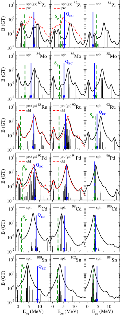
Figure 3: (Color online) Same as in Fig. 2, but for Zr, Mo, Ru, Pd, Cd, and Sn isotopes.

The phase space factors increase with $Q_{if}$ and thus the decay rates are more sensitive to the strength $B_{if}$ located at low excitation energies of the daughter nucleus. It is also interesting to notice the relative importance of both $\beta^{+}$ decay and electron capture phase space factors (see Fig. 3 in Ref.sarri_plb ). In general, the former dominates at sufficiently high $Q_{if}$ (low excitation energies in the daughter nucleus), while the latter is always dominant at sufficiently low $Q_{if}$ (high excitation energies in the daughter nucleus).

The $\beta$-decay half-life in the laboratory is obtained by summing all the allowed transition strengths to states in the daughter nucleus with excitation energies lying below the corresponding $Q_{EC}$ energy, and weighted with the phase space factors,

$$T_{1/2}^{-1}=\frac{\lambda}{\ln 2}=\frac{1}{D}\sum_{0<E_{f}<Q_{EC}}\left[B_{if}(GT)+B_{if}(F)\right]\Phi_{if}^{\beta^{+}/oEC}\,,$$ (25)

where the $Q_{EC}$ energy is given by

$$Q_{EC}=M_{p}-M_{d}+m_{e}=Q_{\beta^{+}}+2m_{e}\,.$$ (26)

III Results for weak decay rates

In this section we present first the results for the potential energy curves. Then, we show the results for the decay properties, GT strength distributions and $\beta$-decay half-lives, under terrestrial conditions comparing them with the available experimental information. Finally, we present the results for the stellar weak decay rates under density and temperature conditions implied in the $rp$ process.

III.1 Potential Energy Curves

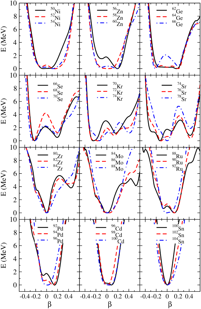
Figure 1: (Color online) Potential energy curves for the even-even isotopes considered in this work obtained from constrained HF+BCS calculations with the Skyrme force SLy4.

In Fig. 1 we can see the potential energy curves for the even-even Ni, Zn, Ge, Se, Kr, Sr, Zr, Mo, Ru, Pd, Cd, and Sn nuclei in the vicinity of the $N=Z$ isotopes considered in this work. We show the energies relative to that of the ground state plotted as a function of the quadrupole deformation $\beta$ in Eq. (5). They are obtained from constrained HF+BCS calculations with the Skyrme force SLy4 sly4 .

The nuclei studied here cover a whole proton shell ranging from magic number $Z=28$ (Ni isotopes) up to magic number $Z=50$ (Sn isotopes). The isotopes considered are the predicted WP nuclei, which in most cases correspond to $N=Z$, and their neighbor isotopes.

Then, it is expected that the lighter and heavier nuclei close to $Z=28$ and $Z=50$, respectively, have a tendency to be spherical. The spherical shapes in these isotopes show sharply peaked profile that become shallow minima as one moves away from $Z=28$ or $Z=50$, and finally deformed shapes are developed as one approaches mid-shell nuclei. The profiles of the latter exhibit a rich structure giving raise to shape coexistence when various minima at close energies are located at different deformations.

It is also worth mentioning the correlations observed between mirror nuclei interchanging the number of neutrons and protons. Thus, we see the remarkable similarity between the profiles of ⁶⁶Ge $(Z=32,N=34)$ and ⁶⁶Se $(Z=34,N=32)$, between ⁷⁰Se $(Z=34,N=36)$ and ⁷⁰Kr $(Z=36,N=34)$, and between ⁷⁴Kr $(Z=36,N=38)$ and ⁷⁴Sr $(Z=38,N=36)$.

These results are in qualitative agreement with similar ones obtained in this mass region from different theoretical approaches. Just to give some examples, shape transition and shape coexistence were discussed in $A\sim 80$ nuclei within a configuration-dependent shell-correction approach based on a deformed Woods-Saxon potential naza85 . Relativistic mean field calculations in this mass region have also been reported in Ref. relat . Nonrelativistic calculations are also available from both Skyrme nonrel_skyrme_1 ; nonrel_skyrme_2 ; nonrel_skyrme_3 and Gogny nonrel_gogny forces, as well as from the complex VAMPIR approach petrovici .

Experimental evidence of shape coexistence in this mass region has become available in the last years wood ; piercey ; chandler ; becker ; fisher ; bouchez ; gade ; gorgen05 ; clement ; davies ; andreoiu ; singh ; hurst ; gorgen07 ; ljungvall ; obertelli , and by now this is a well established characteristic feature in the neutron-deficient $A=70-80$ mass region.

III.2 Laboratory Gamow-Teller strength and half-lives

While the half-lives give only a limited information of the decay (different strength distributions may lead to the same half-life), the strength distribution contains all the information. It is of great interest to study the decay rates under stellar $rp$ conditions using a nuclear structure model that reproduces the strength distributions and half-lives under terrestrial conditions.

In the next figures, we show the results obtained for the energy distributions of the GT strength corresponding to the equilibrium shapes for which we obtained minima in the potential energy curves in Fig. 1. The GT strength is plotted versus the excitation energy of the daughter nucleus $E_{ex}=E_{f}$ (MeV).

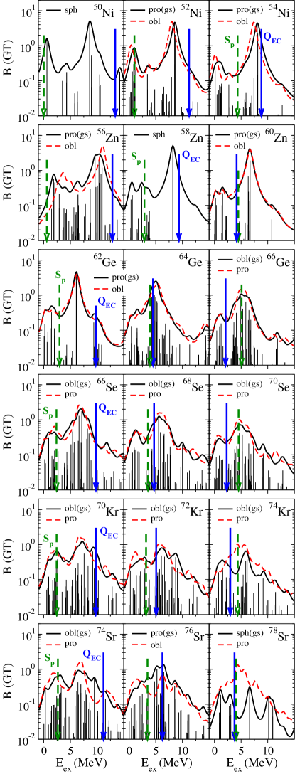
Figure 2: (Color online) Calculated GT strength distributions for Ni, Zn, Ge, Se, Kr, and Sr isotopes obtained from their ground states, as well as from the shape coexisting states. The individual strengths correspond to the ground states, whereas folded distributions are shown for the various configurations considered in each isotope. $Q_{EC}$ values and proton separation energies $S_{p}$ are shown by vertical lines.

Fig. 2 (3) contains the results for the isotopes Ni, Zn, Ge, Se, Kr, and Sr (Zr, Mo, Ru, Pd, Cd, and Sn). We show the energy distributions of the individual GT strengths in the case of the ground state shapes. We also show the continuous distributions for both ground state and possible shape isomers, obtained by folding the strength with 1 MeV width Breit-Wigner functions. The vertical arrows show the $Q_{EC}$ energy, as well as the proton separation energy in the daughter nucleus, both taken from experiment audi .

It is worth noticing that in general both deformations produce quite similar GT strength distributions on a global scale. The main exceptions correspond to the comparison between spherical and deformed shapes, where clear differences can be observed. In any case, the small differences among the various shapes at the low energy tails (below the $Q_{EC}$) of the GT strength distributions lead to sizable effects in the $\beta$-decay half-lives. These differences can be better seen because of the logarithmic scale.

Experimental information on GT strength distributions are mainly available for ⁷²Kr piqueras , ⁷⁴Kr poirier , ⁷⁶Sr nacher , and ^102,104Sn karny isotopes, where $\beta^{+}$-decay experiments have been performed with total absorption spectroscopy techniques, allowing the extraction of the GT strength in practically the whole $Q$-energy window. In Ref. sarri_prc a comparison between similar calculations to those in this work and the experimental data for Kr and Sr isotopes was carried out. In general, good agreement with experiment was found and this was one of the reasons to extrapolate this type of calculations to stellar environments, as well as to other WP nuclei.

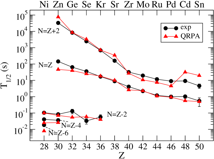
Figure 4: (Color online) Calculated QRPA half-lives compared to experimental values.

Measurements of the decay properties (mainly half-lives) of nuclei in this mass region have been reported in the last years karny ; oinonen ; kienle ; faestermann ; wohr ; kankainen ; kavatsyuk ; dossat ; bazin ; stoker ; weber ; elomaa . The calculation of the half-lives in Eq.(25) involves the knowledge of the GT strength distribution and of the $Q_{EC}$ values. In this work experimental values for $Q_{EC}$ are used. They are taken from Ref. audi or from the Jyväskylä mass database weber ; jyvaskyla , when available. In Fig. 4 the measured half-lives are compared to the QRPA results obtained from the equilibrium deformations of the various isotopes. In general good agreement for the $N=Z$ WP is obtained. Also for the more stable $N=Z+2$ the agreement is very reasonable, except for the heavier Cd an Sn isotopes, where the half-lives are overestimated. The half-lives of the more exotic isotopes are fairly well described by QRPA.

III.3 Stellar weak decay rates

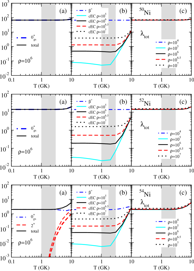
Figure 5: (Color online) Decay rates ($s^{-1}$)of ^50,52,54Ni isotopes as a function of the temperature $T$ (GK). (a) Decomposition of the total rates into their contributions from the decays of the ground and excited $2^{+}$ states. (b) Decomposition of the rates into their $\beta^{+}$ and $cEC$ components evaluated at different densities. (c) Total rates at various densities. The label $\rho$ stands for $\rho Y_{e}$ (mol/cm³) (see text).

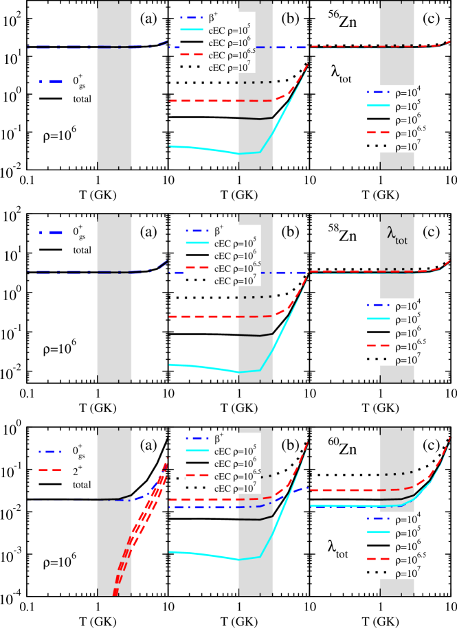
Figure 6: (Color online) Same as in Fig. 5, but for ^56,58,60Zn isotopes.

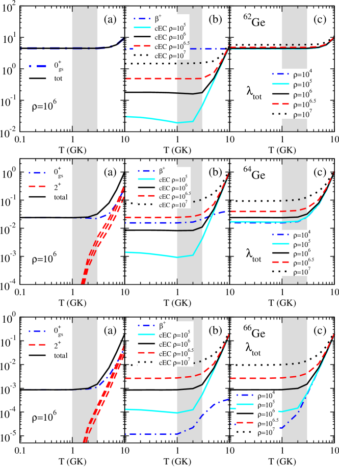
Figure 7: (Color online) Same as in Fig. 5, but for ^62,64,66Ge isotopes.

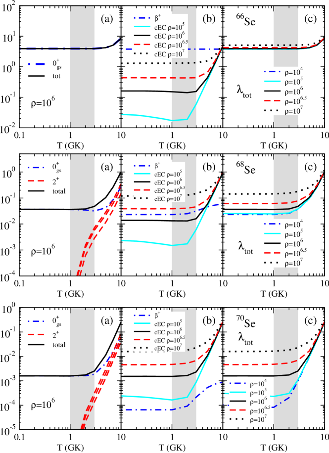
Figure 8: (Color online) Same as in Fig. 5, but for ^66,68,70Se isotopes.

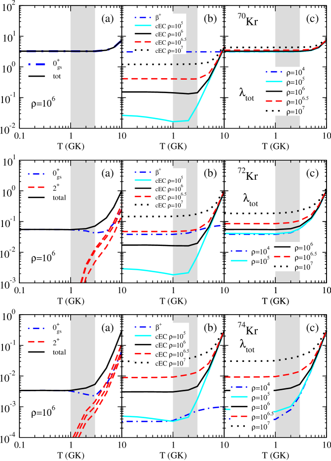
Figure 9: (Color online) Same as in Fig. 5, but for ^70,72,74Kr isotopes.

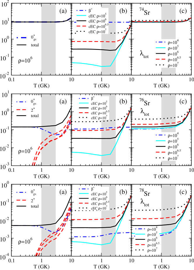
Figure 10: (Color online) Same as in Fig. 5, but for ^74,76,78Sr isotopes.

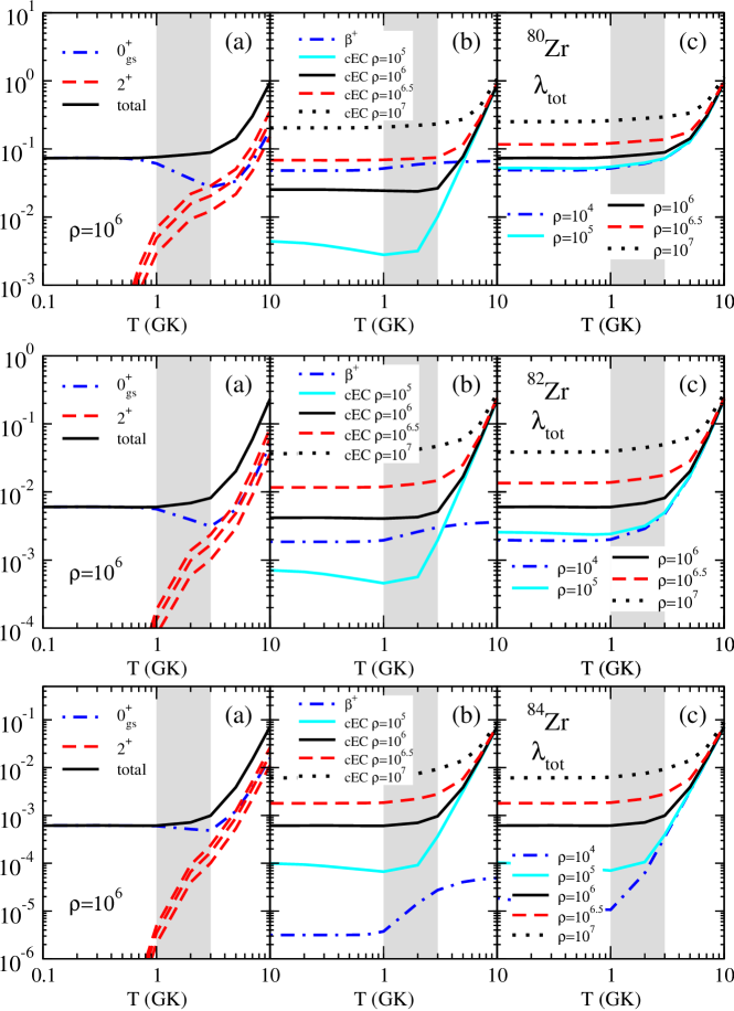
Figure 11: (Color online) Same as in Fig. 5, but for ^80,82,84Zr isotopes.

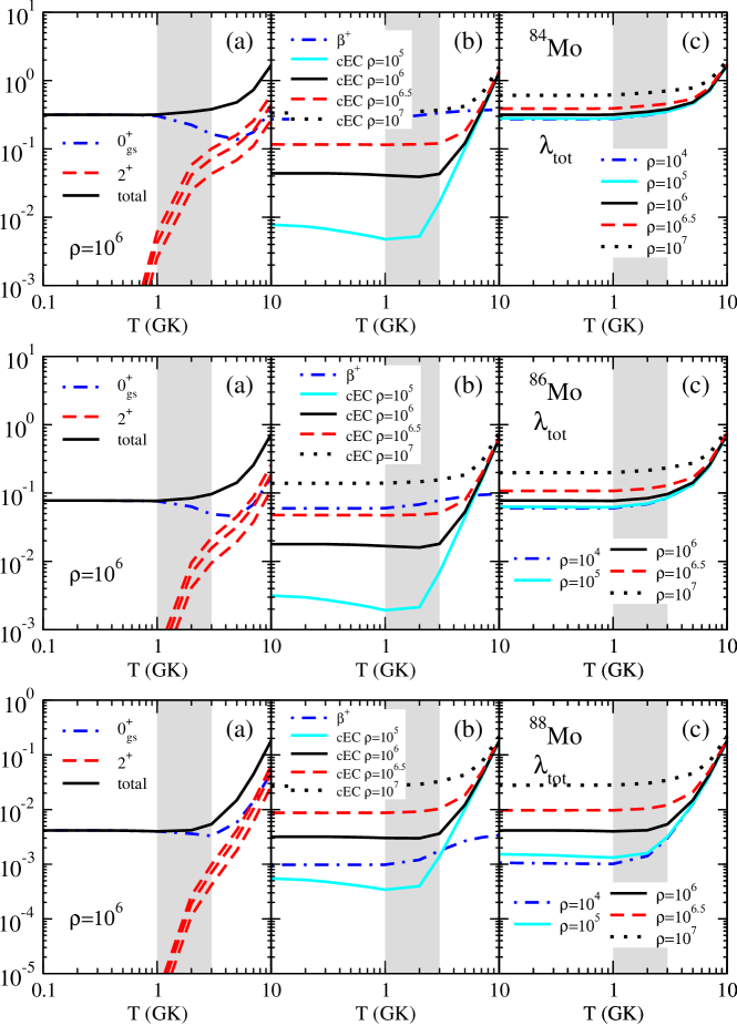
Figure 12: (Color online) Same as in Fig. 5, but for ^84,86,88Mo isotopes.

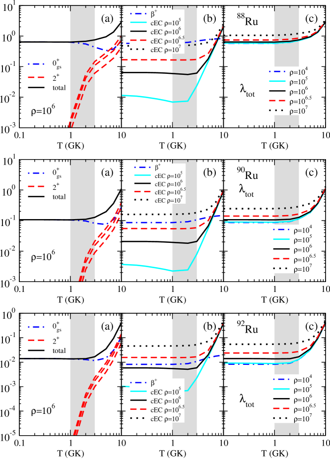
Figure 13: (Color online) Same as in Fig. 5, but for ^88,90,92Ru isotopes.

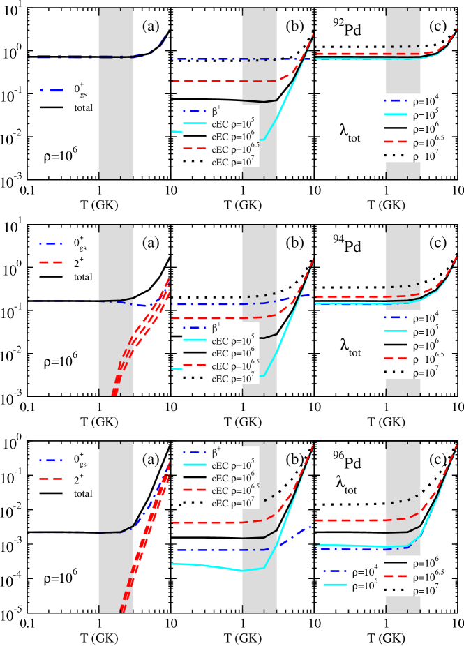
Figure 14: (Color online) Same as in Fig. 5, but for ^92,94,96Pd isotopes.

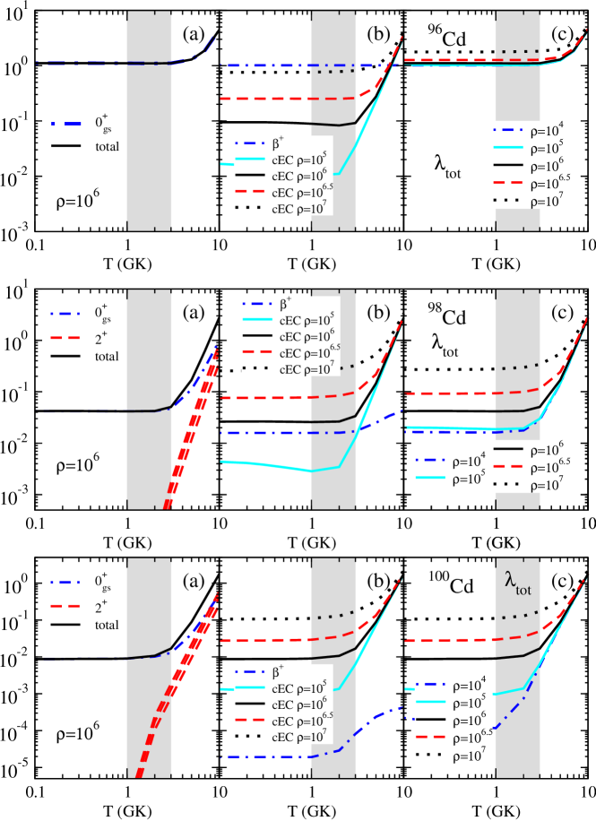
Figure 15: (Color online) Same as in Fig. 5, but for ^96,98,100Cd isotopes.

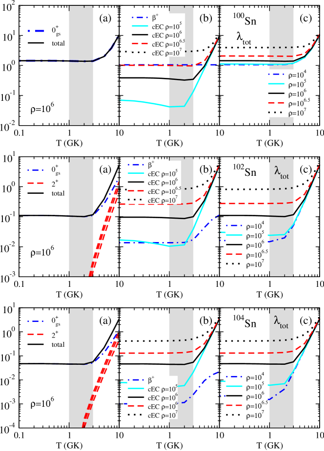
Figure 16: (Color online) Same as in Fig. 5, but for ^100,102,104Sn isotopes.

Figures 5-16 show the decay rates as a function of the temperature $T$. On the left-hand side (a) one can see the decomposition of the total rates into their contributions from the decay of the the ground state $0^{+}_{\rm gs}\rightarrow 1^{+}$ and from the decay of the excited state $2^{+}\rightarrow 1^{+},2^{+},3^{+}$ in the parent nucleus. The middle panel (b) contains the decomposition of the rates into their $\beta^{+}$ and $cEC$ components evaluated at various densities ($\rho Y_{e}$). On the right-hand side (c) the total rates for various densities are presented. The gray area is the relevant range $T=1-3$ GK for the $rp$ process. Each figure contains the results for three isotopes. The results corresponding to the more exotic ones are displayed on top, whereas the results corresponding to the more stable isotopes appear on the bottom. In the middle we find the intermediate isotopes, which in most cases correspond to the WP nuclei.

The results decomposed into their contributions from various parent states (a) show that the decay from the ground state is always dominant at the temperatures within the gray area of interest. The contributions of the decays from excited states increase with $T$, as they become more and more thermally populated, but in general they do not represent significant contributions to the total rates and can be neglected in most cases. Nevertheless, there are a few cases where these contributions should not be ignored, which correspond to those cases where the excitation energy of the $2^{+}$ excited state is very low. This is the case of the middle-shell nuclei Kr, Sr, Zr, and Mo, where the contributions of the low-lying excited states compete with those of the ground state already at temperatures in the range of $rp$ process. The effect on the rates of the decay from excited $0^{+}_{2}$ states was also considered in Ref. sarri_plb in the case of Kr and Sr isotopes. It was concluded that in general their relative impact is again very small in the total rates at these temperatures.

Concerning the competition between $\beta^{+}$ and $cEC$ rates (b) one should distinguish between different isotopes. Thus, the more exotic isotopes appearing on the top of the figures show a clear dominance of the $\beta^{+}$ rates over the $cEC$ ones that can be neglected except at very high densities beyond $rp$-process conditions. On the other hand, the opposite is true with respect to the more stable isotopes on the bottom, where the $\beta^{+}$ rates are completely negligible. The origin of these features can be understood from the behavior of the phase space factors as a function of the available energy $Q_{if}$. As it was mentioned above and discussed in Ref. sarri_plb , more exotic nuclei with larger $Q_{if}$ values favor $\beta^{+}$ because of the larger phase space factors, while the opposite is true for more stable nuclei with smaller $Q_{if}$ values.

The interesting cases occur in the middle panels that correspond in most cases to the $N=Z$ WP nuclei. Here, there is a competition between $\beta^{+}$ and $cEC$ rates that depends on the nucleus, on the temperature, and on the density $\rho Y_{e}$. One can see that for large enough densities, $cEC$ becomes dominant at any $T$. For low densities, $\beta^{+}$ rates dominate at low $T$, while $cEC$ dominates at higher $T$, but in general there is a competition that must be analyzed case by case.

Finally, the total rates in (c) are a consequence of the competition between $\beta^{+}$ and $cEC$ rates mentioned above. Since the $\beta^{+}$ decay rate is independent of the density and depends on $T$ only through the contributions from excited parent states, the total rates are practically constant for the more exotic isotopes in the upper figures, only modulated by the small contribution from $cEC$. In the central isotopes the rates are the result of the competition discussed in (b), and finally in the heavier isotopes (lower figures) we can see that the total rates are practically due to $cEC$ with little contribution from $\beta^{+}$. Tables containing $\beta^{+}$, $cEC$, and total decay rates for all the isotopes considered in this work are available in Ref. epaps .

IV Summary and Conclusions

In summary, the weak decay rates of waiting point and neighbor nuclei from Ni up to Sn have been investigated at temperatures and densities where the $rp$ process takes place. The nuclear structure has been described within a microscopic QRPA approach based on a selfconsistent Skyrme-Hartree-Fock-BCS mean field that includes deformation. This approach reproduces both the experimental half-lives and the more demanding GT strength distributions measured under terrestrial conditions in this mass region.

The relevant ingredients to describe the rates have been analyzed. We have studied the contributions to the decay rates coming from excited states in the parent nucleus which are populated as $T$ raises. It is found that they start to play a role above $T=1-2$ GK and that for isotopes with low-lying excited states, their contributions can be comparable to those of the ground states. Concerning the contributions from the continuum electron capture rates, it is found that they are enhanced with $T$ and $\rho$. They are already comparable to the $\beta^{+}$ decay rates at $rp$ conditions for the WP nuclei. For more exotic isotopes the rates are dominated by $\beta^{+}$ decay, while for more stable isotopes they are dominated by $cEC$.

- (1) K. Langanke and G. Martínez-Pinedo, Rev. Mod. Phys. 75, 819 (2003).
- (2) A. Aprahamian, K. Langanke, and M. Wiescher, Prog. Part. Nucl. Phys. 54, 535 (2005).
- (3) R. K. Wallace and S. E. Woosley, Ap. J. Suppl. 45, 389 (1981).
- (4) F.-K. Thielemann et al., Nucl. Phys. A 570, 329c (1994).
- (5) H. Schatz et al., Phys. Rep. 294, 167 (1998).
- (6) S. E. Woosley et al., Ap. J. Suppl. 151, 75 (2004).
- (7) L. Van Wormer et al., Ap. J. 432, 326 (1994).
- (8) J. Pruet and G.M. Fuller, Ap. J. Suppl. 149, 189 (2003).
- (9) H. Schatz et al., Phys. Rev. Lett. 86, 3471 (2001).
- (10) G. M. Fuller, W. A. Fowler and M. J. Newman, Ap. J. Suppl. 42, 447 (1980); Ap. J. 252, 715 (1982); Ap. J. Suppl. 48, 279 (1982); Ap. J. 293, 1 (1985).
- (11) S. Wanajo, Ap. J. 647, 1323 (2006).
- (12) C. Fröhlich et al., Phys. Rev. Lett. 96, 142502 (2006).
- (13) K. Langanke and G. Martínez-Pinedo, Nucl. Phys. A673, 481 (2000).
- (14) K. Langanke and G. Martínez-Pinedo, At. Data Nucl. Data Tables 79, 1 (2001).
- (15) J.-U. Nabi and H. V. Klapdor-Kleingrothaus, At. Data Nucl. Data Tables 71, 149 (1999); 88, 237 (2004).
- (16) N. Paar, G. Colò, E. Khan, and D. Vretenar, Phys. Rev. C 80, 055801 (2009).
- (17) P. Sarriguren, Phys. Lett. B 680, 438 (2009).
- (18) P. Sarriguren, Phys. Rev. C 79, 044315 (2009).
- (19) Evaluated Nuclear Structure Data File (ENSDF), http://www.nndc.bnl.gov/ensdf/.
- (20) J. Krumlinde and P. Möller, Nucl. Phys. A417, 419 (1984); P. Möller and J. Randrup, Nucl. Phys. A514, 1 (1990).
- (21) F. Frisk, I. Hamamoto, and X. Z. Zhang, Phys. Rev. C 52, 2468 (1995).
- (22) P. Möller, J. R. Nix, and K. -L. Kratz, At. Data Nucl. Data Tables 66, 131 (1997).
- (23) M. Hirsch, A. Staudt, K. Muto and H.V. Klapdor-Kleingrothaus, Nucl. Phys. A535, 62 (1991); K. Muto, E. Bender, T. Oda, and H.V. Klapdor-Kleingrothaus, Z. Phys. A 341, 407 (1992).
- (24) H. Homma, E. Bender, M. Hirsch, K. Muto, H. V. Klapdor-Kleingrothaus and T. Oda, Phys. Rev. C 54, 2972 (1996).
- (25) I. N. Borzov, Nucl. Phys. A 777, 645 (2006).
- (26) N. Paar, T. Nikšić, D. Vretenar, and P. Ring, Phys. Rev. C 69, 054303 (2004).
- (27) S. Fracasso and G. Colò, Phys. Rev. C 76, 044307 (2007).
- (28) A. Petrovici, K. W. Schmid, O. Radu, and A. Faessler, Nucl. Phys. A799, 94 (2008); Phys. Rev. C 78, 044315 (2008); A. Petrovici, K. W. Schmid, O. Andrei, and A. Faessler, Phys. Rev. C 80, 044319 (2009).
- (29) P. Sarriguren, E. Moya de Guerra, A. Escuderos, and A. C. Carrizo, Nucl. Phys. A635, 55 (1998).
- (30) P. Sarriguren, E. Moya de Guerra, and A. Escuderos, Nucl. Phys. A691, 631 (2001).
- (31) P. Sarriguren, E. Moya de Guerra, and A. Escuderos, Phys. Rev. C 64, 064306 (2001).
- (32) E. Chabanat et al., Nucl. Phys. A635, 231 (1998).
- (33) D. Vautherin, Phys. Rev. C 7, 296 (1973).
- (34) G. Audi, O. Bersillon, J. Blachot, and A. H. Wapstra, Nucl. Phys. A729, 3 (2003).
- (35) H. Flocard, P. Quentin, A. K. Kerman, and D. Vautherin, Nucl. Phys. A203, 433 (1973).
- (36) P. Sarriguren, E. Moya de Guerra, and A. Escuderos, Nucl. Phys. A658, 13 (1999).
- (37) P. Sarriguren, O. Moreno, R. Álvarez-Rodríguez, and E. Moya de Guerra, Phys. Rev. C 72, 054317 (2005).
- (38) P. Sarriguren, R. Álvarez-Rodríguez, and E. Moya de Guerra, Eur. Phys. J. A 24, 193 (2005).
- (39) P. Sarriguren and J. Pereira, Phys. Rev. C 81, 064314 (2010).
- (40) A. Bohr and B. Mottelson, Nuclear Structure, (Benjamin, New York 1975).
- (41) M. S. Antony, A. Pape, and J. Britz, At. Data Nucl. Data tables 66, 1 (1997).
- (42) N.B. Gove and M.J. Martin, Nucl. Data Tables 10, 205 (1971).
- (43) W. Nazarewicz, J. Dudek, R. Bengtsson, T. Bengtsson, and I. Ragnarsson, Nucl. Phys. A435, 397 (1985).
- (44) G. A. Lalazissis and M. M. Sharma, Nucl. Phys. A 586, 201 (1995); G. A. Lalazissis, S. Raman, and P. Ring, At. Data Nucl. Data Tables 71, 1 (1999).
- (45) P. Bonche, H. Flocard, P.-H. Heenen, S. J. Krieger, and M. S. Weiss, Nucl. Phys. A443, 39 (1985).
- (46) M. Bender, P. Bonche and P.-H. Heenen, Phys. Rev. C 74, 024312 (2006).
- (47) M. Yamagami, K. Matsuyanagi, and M. Matsuo, Nucl. Phys. A693, 579 (2001).
- (48) S. Hilaire and M. Girod, Eur. Phys. J. A 33, 237 (2007); M. Girod, J.-P. Delaroche, A. Görgen, and A. Obertelli, Phys. Lett. B 676, 39 (2009).
- (49) A. Petrovici, K. W. Schmid, and A. Faessler, Nucl. Phys. A605, 290 (1996); A665, 333 (2000).
- (50) J. L. Wood, E. F. Aganjar, C. de Coster and K. Heyde, Nucl. Phys. A651, 323 (1999).
- (51) R. B. Piercey et al., Phys. Rev. Lett. 47, 1514 (1981).
- (52) C. Chandler et al., Phys. Rev. C 56, R2924 (1997).
- (53) F. Becker et al., Eur. Phys. J. A 4, 103 (1999).
- (54) S. M. Fischer et al., Phys. Rev. Lett. 84, 4064 (2000).
- (55) E. Bouchez et al., Phys. Rev. Lett. 90, 082502 (2003).
- (56) A. Gade et al., Phys. Rev. Lett. 95, 022502 (2005).
- (57) A. Görgen et al., Eur. Phys. J. A 26, 153 (2005).
- (58) E. Clément et al., Phys. Rev. C 75, 054313 (2007).
- (59) P. J. Davies et al., Phys. Rev. C 75, 011302(R) (2007).
- (60) C. Andreoiu et al., Phys. Rev. C 75, 041301(R) (2007).
- (61) B. S. Nara Singh et al., Phys. Rev. C 75, 061301(R) (2007).
- (62) A. M. Hurst et al., Phys. Rev. Lett. 98, 072501 (2007).
- (63) A. Görgen et al., Eur. Phys. J. Special Topics 150, 117 (2007).
- (64) J. Ljungvall et al., Phys. Rev. Lett. 100, 102502 (2008).
- (65) A. Obertelli et al., Phys. Rev. C 80, 031304(R) (2009).
- (66) I. Piqueras et al., Eur. Phys. J. A 16, 313 (2003).
- (67) E. Poirier et al., Phys. Rev. C 69, 034307 (2004).
- (68) E. Nácher et al., Phys. Rev. Lett. 92, 232501 (2004).
- (69) M. Karny et al., Eur. Phys. J. A 27, 129 (2006).
- (70) M. Oinonen et al., Phys. Rev. C 61, 035801 (2000).
- (71) P. Kienle et al., Prog. Part. Nucl. Phys. 46, 73 (2001).
- (72) T. Faestermann et al., Eur. Phys. J. A 15, 185 (2002).
- (73) A. Wöhr et al., Nucl. Phys. A 742, 349 (2004).
- (74) A. Kankainen et al., Eur. Phys. J. A 29, 271 (2006).
- (75) O. Kavatsyuk et al., Eur. Phys. J. A 31, 319 (2007).
- (76) C. Dossat et al., Nucl. Phys. A 792, 18 (2007).
- (77) D. Bazin et al., Phys. Rev. Lett. 101, 252501 (2008).
- (78) J. B. Stoker et al., Phys. Rev. C 79, 015803 (2009).
- (79) C. Weber et al., Phys. Rev. C 78, 054310 (2008).
- (80) V.-V. Elomaa et al., Eur. Phys. J. A 40, 1 (2009); Phys. Rev. Lett. 102, 252501 (2009).
- (81) http://research.jyu.fi/igisol/JYFLTRAP_masses/
- (82) See supplementary material at [] for text files containing weak-decay rates in a grid of densities () and temperatures () covering the rp-process conditions.