Desynchronization transitions in nonlinearly coupled phase oscillators

Abstract

We consider the nonlinear extension of the Kuramoto model of globally coupled phase oscillators where the phase shift in the coupling function depends on the order parameter. A bifurcation analysis of the transition from fully synchronous state to partial synchrony is performed. We demonstrate that for small ensembles it is typically mediated by stable cluster states, that disappear with creation of heteroclinic cycles, while for a larger number of oscillators a direct transition from full synchrony to a periodic or quasiperiodic regime occurs.

1 Introduction

A model of coupled limit cycle oscillators explains a variety of natural phenomena in various fields of science. The applications range from the description of the collective dynamics of Josephson junctions [1], lasers [2], and electrochemical oscillators [3] to neuronal populations [4], etc. Very often, when the oscillator network is not too sparse, it can be approximately considered as fully connected, or globally coupled.

Ensembles of weakly interacting units are successfully treated within the framework of phase approximation [5, 6, 7]. Most popular is the Kuramoto model of sine-coupled phase oscillators, or its extension, the Kuramoto-Sakaguchi model [8]. This model explains self-synchronization and appearance of a collective mode (mean field) in an ensemble of generally non-identical elements; the transition to synchrony occurs at a certain critical value of the coupling constant that is roughly proportional to the width of the distribution of natural frequencies [5, 6, 9, 10].

An extension of the Kuramoto model for the case of nonlinear coupling has been suggested in our recent publications [11, 12], see also [13, 14]. Nonlinearity in this context means that the effect of the collective mode on an individual unit depends on the amplitude of this mode, so that, e.g., the interaction of the field and of a unit can be attractive for a weak field and repulsive for a strong one. Formally, this is represented by the dependence of the parameters of the Kuramoto-Sakaguchi model (the coupling strength and the phase shift) on the mean field amplitude. The model exhibits nontrivial effects like a destruction of a completely synchronous state and appearance of partial synchrony in an ensemble of identical units. Moreover, in this setup the frequencies of the collective mode and of oscillators can be different and incommensurate.

An analytical description of the dynamics of oscillator ensembles remains an important and challenging problem. A seminal work in this direction is that of Watanabe and Strogatz (WS) [15, 16]. The WS theory is a powerful tool that provides a nearly full dynamical description of ensembles of identical oscillators, sine-coupled to a common external force. In particular, this force can be the mean field of the population, so that for the case of identical units the WS theory almost completely describes the Kuramoto-Sakaguchi and the nonlinear models (see [12]). This description is given in terms of three collective (macroscopic) variables, hereafter called the WS variables, plus constants of motion. The collective variables obey $3$ WS equations (see [17]); thus, the dynamics of an ensemble of identical elements is effectively $3$-dimensional. However, the WS theory has one drawback: it cannot describe certain cluster states, i.e. regimes where the oscillators build identical groups. In this paper we complement the WS theory by performing a direct bifurcation analysis of the dynamical phase equations of the model of nonlinearly coupled phase oscillators. We will especially emphasis on cluster states and their bifurcations, in particular on the heteroclinic cycles (see [18] for a recent review of robust heteroclinic cycles) that can be hardly treated within the WS approach. We will see that the role of clusters is mostly important for small ensembles. Because of identity of the oscillators, the system possesses a permutation symmetry, so we employ the corresponding bifurcation approach (see, e.g., [19, 20]).

The paper is organized as follows. We introduce the basic model in Section 2. Then in Section 3 we discuss general properties of bifurcations, possible attractors and their interpretation as different synchronization patterns. In Section 4 we present bifurcation diagrams for a model of nonlinearly coupled oscillators with quadratic nonlinearity [12]. In Conclusion a relation to the WS theory is discussed.

2 Model of nonlinearly coupled phase oscillators

We consider an ensemble of $N$ limit cycle oscillators, described by their phases $\theta_{i}\in[0,2\pi)$, $i=1,\ldots,N$. They are assumed to interact globally, via the complex mean field

$$re^{i\psi}=\frac{1}{N}\sum_{j=1}^{N}e^{i\theta_{j}}\;,$$ (1)

having amplitude $r$ and phase $\psi$:

$$\dot{\theta}_{i}=\omega_{i}+G(r,\psi,\theta_{i})\;.$$ (2)

Here $\omega_{i}$ are natural frequencies of the oscillators and $G$ is the coupling function. Different popular models correspond to different choices of coupling function $G$. The case $G(r,\psi,\theta_{i})=rK\text{Im}(e^{i(\psi-\theta)})$ corresponds to the famous Kuramoto model [6], while the choice $G(r,\psi,\theta_{i})=rK\text{Im}(e^{-i\alpha}e^{i(\psi-\theta)})$ yields the Kuramoto-Sakaguchi model [8].

In this paper we focus on a coupling function that nonlinearly depends on the amplitude of the mean field $r$ and on a set of parameters $\beta$:

$$G(r,\psi,\theta_{i})=rK(r,\beta)\sin(\psi-\theta+\alpha(r,\beta))\;.$$ (3)

This model has been introduced in  [11] and studied in the thermodynamic limit $N\to\infty$ in [12]. In this paper we focus on the properties of small ensembles of nonlinearly coupled oscillators, restricting our analysis to the case of identical oscillators $\omega_{i}=\omega$ and of phase nonlinearity only $K(r,\beta)=1$. The latter restriction is not very important, as the cases where $K(r,\beta)$ can change sign are in fact trivial. Substituting (3) in (2) we obtain an equivalent formulation of the ensemble dynamics

$$\dot{\theta}_{i}=\omega+\frac{1}{N}\sum_{j=1}^{N}\sin(\theta_{j}-\theta_{i}+\alpha(r,\beta))\;.$$ (4)

To exploit the phase-shift symmetry of this system one can describe the system dynamics in terms of the phase differences

$$\varphi_{i}=\theta_{1}-\theta_{i+1},\quad i=1,\dots,N-1,$$ (5)

thus reducing this $N$-dimensional system to the $(N-1)$-dimensional system

$$\dot{\varphi}_{i} =-\frac{1}{N}\left[\sum\limits_{j=1,j\not=i}\limits^{N-1}\sin(\varphi_{i}-\varphi_{j}+\alpha(r,\beta))+\right.$$ (6)

$$\left.+\sin(\varphi_{i}+\alpha(r,\beta))+\sum\limits_{j=1}\limits^{N-1}\sin(\varphi_{j}-\alpha(r,\beta))\right]\;.$$

One can check that order parameter $r$ can be written in phase differences as

$$r=\frac{1}{N}\sqrt{N+2\sum_{i,j=1,i\not=j}^{N-1}(\cos(\varphi_{j})+\cos(\varphi_{i}-\varphi_{j}))}\;.$$ (7)

Below we will discuss synchronization transitions in the system studying invariant manifolds, fixed points, cycles, heteroclinic cycles and their bifurcations for the system in phase differences (6).

Before proceeding to the analysis, we mention that system (4) possesses symmetries given by all permutations of the oscillators [21]. Due to identity of the oscillators, the main dynamical regimes appear as invariant sets of the system:
1) Completely synchronous solution, where all the oscillators are in the same state:

$$\mathcal{O}=\{(\theta_{1},\cdots,\theta_{N})~{}:~{}\theta_{1}=\theta_{2}=\dots=\theta_{N}\};$$

3) Completely asynchronous solution

$$\mathcal{M}=\left\{(\theta_{1},...,\theta_{N}):\ \sum\limits_{j=1}^{N}e^{i\theta_{j}}=0\right\}.$$ (8)

The set $\mathcal{M}$ is a union of invariant manifolds of dimension $N-2$ for $N\geq 3$ [22], it corresponds to the case of vanishing order parameter $r=0$.
2) Cluster states, where groups of oscillators have identical phases. A general $n$-cluster state can be written as (up to permutation of indices)

$$\mathcal{P}_{n}=\left\{(\theta_{1},...,\theta_{N}):\theta_{1}=\cdots=\theta_{p_{1}}\,;\theta_{p_{1}+1}=\cdots=\theta_{p_{1}+p_{2}}\,;\cdots\,;\,\theta_{\sum_{1}^{n-1}p_{j}+1}=\cdots=\theta_{N}\right\},$$ (9)

where $p_{1}+p_{2}+\cdots+p_{n}=N$. We will be mainly interested in 2-cluster states (we will see that only such states appear as stationary solutions)

$$\mathcal{P}_{2}=\left\{(\theta_{1},...,\theta_{N}):\theta_{1}=\cdots=\theta_{p}\,;\theta_{p+1}=\cdots=\theta_{N}\right\}\;,$$ (10)

characterized by the partition $(p:N-p)$.

3 General analysis of synchronization and bifurcations

In this section we study general bifurcation scenarios in the system of nonlinearly coupled oscillators (4), to be illustrated by particular examples in the next section.

3.1 Bifurcations in the Kuramoto–Sakaguchi model

We start with the simplest case of linearly coupled oscillators. Here model (4) reduces to the standard Kuramoto-Sakaguchi model which we write as

$$N\dot{\theta}_{i}=g_{i}(\theta_{1},\ldots,\theta_{N},\alpha)=-\sum_{j=1}^{N}\sin(\theta_{i}-\theta_{j}-\alpha)$$ (11)

Equilibria.

To describe the steady states of the corresponding system in differences $\varphi_{i}=\theta_{1}-\theta_{1+i}$, we need to solves the system of $N-1$ algebraic equations

$$g_{1}(\theta_{1},\dots,\theta_{N},\alpha)-g_{i}(\theta_{1},\dots,\theta_{N},\alpha)=0,\quad i=2,\cdots,N,$$ (12)

where $\alpha$ is a scalar parameter. The next lemma helps us to characterize the steady states of the system (11).

Lemma 1

For any $\alpha\in\mathbb{T}^{1}$, the set $(\theta_{1},\cdots,\theta_{N})$ satisfies system of equations (12) if and only if one of the following three conditions is fulfilled:
1) $\theta_{1}=\cdots=\theta_{N}$,
2) $\sum_{j=1}^{N}e^{i\theta_{j}}=0$,
3) $\theta_{1}=\theta_{2}=\cdots=\theta_{p}\not=\theta_{p+1}=\theta_{p+2}=\cdots=\theta_{N},\quad p=1,\cdots,N-1$, (plus all possible permutations).

This Lemma means that the only possible steady states are that of complete synchrony (one cluster), complete asynchrony, and of two clusters.

Proof:  It is easy to check that states 1) – 3) satisfy the system (12). We will show that the roots of the system (12) satisfy 1) – 3). We can re-write (12) in the following way:

$$(\sin(\theta_{1}-\alpha)-\sin(\theta_{i}-\alpha))\sum_{j=1}^{N}\cos\theta_{j}-(\cos(\theta_{1}-\alpha)-\cos(\theta_{i}-\alpha))\sum_{j=1}^{N}\sin\theta_{j}=0,$$ (13)

where $i=2,\dots,N$. We consider four possible cases.
A. If $\sum_{j=1}^{N}\sin\theta_{j}=0$ and $\sum_{j=1}^{N}\cos\theta_{j}=0$ simultaneously, then the condition 2) of the lemma satisfies.
B. The next possible case is that of $\sum_{j=1}^{N}\sin\theta_{j}=0$ but $\sum_{j=1}^{N}\cos\theta_{j}\not=0$. In this case (13) implies

$$\sin(\theta_{1}-\alpha)=\sin(\theta_{i}-\alpha),\quad i=2,\dots,N.$$

The last system shows that we can obtain only two–cluster solutions:

$$\theta_{i}=\left\{\begin{array}[]{ll}\theta_{1},&\ i=2,\dots,p,\\[5.69054pt] -\theta_{1}+2\alpha+\pi,&\ i=p+1,\dots,N,\end{array}\right.$$

which must satisfy equations

$$p\sin\theta_{1}-(N-p)\sin(\theta_{1}-2\alpha)=0,\quad p=1,\dots,N.$$

The last equations arise from $\sum_{j=1}^{N}\sin\theta_{j}=0$ and they show that two–cluster states are possible only for some values of parameter $\alpha$ in this case. Note that the case $p=N$ corresponds to a one–cluster solution (condition 3 reduces to condition 1).
C. Consider the case, where $\sum_{j=1}^{N}\cos\theta_{j}=0$, and $\sum_{j=1}^{N}\sin\theta_{j}\not=0$. As in the previous case we obtain the possibility of two–cluster (or one–cluster, if $p=N$) states only:

$$\theta_{i}=\left\{\begin{array}[]{ll}\theta_{1},&\ i=2,\dots,p,\\[5.69054pt] -\theta_{1}+2\alpha,&\ i=p+1,\dots,N,\end{array}\right.$$

which satisfy conditions

$$p\cos\theta_{1}+(N-p)\cos(\theta_{1}-2\alpha)=0,\quad p=1,\dots,N.$$

D. Consider $(\theta_{1},\cdots,\theta_{n})$ such that $\sum_{j=1}^{N}\sin\theta_{j}\not=0$ and $\sum_{j=1}^{N}\cos\theta_{j}\not=0$. Denote $S:=\sum_{j=1}^{N}\sin\theta_{j}$, $C:=\sum_{j=1}^{N}\cos\theta_{j}$, $s_{j}^{\alpha}:=\sin(\theta_{j}-\alpha)$, $c_{j}^{\alpha}:=\cos(\theta_{j}-\alpha)$. Then equation (13) has the following form:

$$(s_{1}^{\alpha}-s_{i}^{\alpha})C-(c_{1}^{\alpha}-c_{i}^{\alpha})S=0,\quad i=2,\cdots,N.$$ (14)

D1. Suppose that $s_{1}^{\alpha}-s_{i}^{\alpha}=0$ for all $i=2,\cdots,N$. Then using inequality $S\not=0$ we obtain $c_{1}^{\alpha}-c_{i}^{\alpha}=0$ for $i=2,\cdots,N$. Equalities for $s_{j}^{\alpha}$ and $c_{j}^{\alpha}$ considered together yield $e^{i(\theta_{j}-\alpha)}-e^{i(\theta_{1}-\alpha)}=0$, $j=2,\dots,N$, what means that all the values of $\theta_{j}$, $j=1,\dots,N$, are equal.
D2. Now let us consider another case, when there exists a number $i_{0}$ such that $s_{1}^{\alpha}-s_{i_{0}}^{\alpha}\not=0$. Without loss of generality we can set $i_{0}=2$. Then from the first of equations (14) we obtain

$$C=(c_{1}^{\alpha}-c_{2}^{\alpha})S/(s_{1}^{\alpha}-s_{2}^{\alpha}).$$

Substituting $C$ into the second equation of (14), we get

$$S(s_{1}^{\alpha}-s_{3}^{\alpha})(c_{1}^{\alpha}-c_{2}^{\alpha})/(s_{1}^{\alpha}-s_{2}^{\alpha})-S(c_{1}^{\alpha}-c_{3}^{\alpha})=0.$$

Using conditions $S\not=0$ and $(s_{1}^{\alpha}-s_{2}^{\alpha})\not=0$, we obtain

$$(s_{1}^{\alpha}-s_{3}^{\alpha})(c_{1}^{\alpha}-c_{2}^{\alpha})-(s_{1}^{\alpha}-s_{2}^{\alpha})(c_{1}^{\alpha}-c_{3}^{\alpha})=0,$$

and then

$$(s_{1}^{\alpha}c_{3}^{\alpha}-c_{1}^{\alpha}s_{3}^{\alpha})+(s_{2}^{\alpha}c_{1}^{\alpha}-c_{2}^{\alpha}s_{1}^{\alpha})+(s_{3}^{\alpha}c_{2}^{\alpha}-c_{3}^{\alpha}s_{2}^{\alpha})=0.$$

After returning to the old notations and some transformations, we obtain the expression

$$\sin(\theta_{1}-\theta_{3})+\sin(\theta_{2}-\theta_{1})+\sin(\theta_{3}-\theta_{2})=0,$$

which already does not contain parameter $\alpha$. We provide the last part of the proof by contradiction. The case D supposes that condition 2) is not valid. Now suppose that the conditions 1) and 3) are not satisfied as well. This means that there exists a solution $(\theta_{1},\dots,\theta_{N})$ of the system (13) such that at least three variables $\theta_{i_{1}}$, $\theta_{i_{2}}$, $\theta_{i_{3}}$ of this solution are not equal to each other. Without loss of generality we can set $i_{1}=1$, $i_{2}=2$, $i_{3}=3$ because we can replace variables using permutation (network has $S_{N}$ symmetry). Inequalities $\theta_{1}\not=\theta_{2}$, $\theta_{1}\not=\theta_{3}$, $\theta_{2}\not=\theta_{3}$ imply that

$$\sin(\theta_{1}-\theta_{3})+\sin(\theta_{3}-\theta_{2})+\sin(\theta_{2}-\theta_{1})=$$

$$=-4\sin\left(\frac{\theta_{1}-\theta_{3}}{2}\right)\sin\left(\frac{\theta_{3}-\theta_{2}}{2}\right)\sin\left(\frac{\theta_{2}-\theta_{1}}{2}\right)\not=0$$

This contradiction proves validity of either 1) or 3).
D3. Consider a situation, when $c_{1}^{\alpha}-c_{i_{0}}^{\alpha}\not=0$ for some number $i_{0}$. In the same way as in the previous case D2 we prove that solutions of (13) satisfy one of the conditions 1) or 3).
Lemma is proved.

Corollaries of Lemma 1.

Lemma 1 implies that all steady states of the Kuramoto–Sakaguchi system, in terms of the phase differences, are one-cluster, two-cluster, or completely desynchronized states. As the two-cluster states constitute straight lines (plus those obtained by permutations of the variables)

$$\varphi_{1}=\varphi_{2}=\cdots=\varphi_{p}\not=\varphi_{p+1}=\varphi_{p+2}=\dots=\varphi_{N-1}=0,\quad p=1,\dots,N-1,$$ (15)

all bifurcations of cluster steady states in this case are one–dimensional (in the sense that the normal forms are one-dimensional). Furthermore, to study the existence of nontrivial cluster steady states we only need to solve scalar algebraic equations

$$p\sin(\varphi_{k}-\alpha)+(N-p)\sin(\varphi_{k}+\alpha)-(N-2p)\sin\alpha=0,\quad k=1,\dots,p.$$ (16)

This equation has only two solutions on $T^{1}$: $\varphi_{k}=0$ and

$$\varphi_{k}=\left\{\begin{array}[]{ll}\arccos\left(-\frac{2p(N-p)+(N^{2}-2p(N-p))\cos(2\alpha)}{N^{2}+2p(N-p)(\cos(2\alpha)-1)}\right)&\alpha\in\left[0;\frac{\pi}{2}\right)\cup\left[\pi;\frac{3\pi}{2}\right),\\[14.22636pt] -\arccos\left(-\frac{2p(N-p)+(N^{2}-2p(N-p))\cos(2\alpha)}{N^{2}+2p(N-p)(\cos(2\alpha)-1)}\right)&\alpha\in\left[\frac{\pi}{2};\pi\right)\cup\left[\frac{3\pi}{2};2\pi\right).\end{array}\right.$$ (17)

We can see that a bifurcation in the system (11) occurs only when $\alpha=\pi/2$ and it is transcritical. The bifurcation value of parameter $\alpha$ doesn’t depend on the number of oscillators $N$ or on the cluster partition (number $p$).

Note that in the case of a symmetric partition $N=2p$, equations (16) have a very simple form

$$2p\sin\varphi_{k}\cos\alpha=0.$$

For this partition the only steady states are $\varphi_{k}=0$ or $\varphi_{k}=\pi$, provided $\alpha\not=\pm\pi/2$. There is no any bifurcation on these lines for these values of the parameter. Vice verse, for $\alpha=\pm\pi/2$ the whole two-cluster invariant line in the case of symmetric partition consists of fixed points. These fixed points are degenerate saddles (in the direction of lines with symmetry mentioned) and together with their one–dimensional manifolds they build a set of heteroclinic cycles.

As it follows from lemma 1 and formula (17), the standard Kuramoto model of identical oscillators ($\alpha=0$) and the system with coupling $\alpha=\pm\pi/2$ have a simple structure of the steady states. The standard Kuramoto model has only equilibria of two types: (i) equilibria that compose the manifold $\mathcal{M}$ (with vanishing order parameter) and (ii) equilibria that have coordinates differences $\theta_{j}-\theta_{k}$ equal to $0$ or to $\pm\pi$. In the case $\alpha=\pm\pi/2$ all equilibria satisfy either (i) lie on the manifold $\mathcal{M}$ or (ii) correspond to a completely synchronous state, where $\theta_{j}=\theta_{k}$, $j,k=\overline{1,N}$, and $r=1$.

3.2 Bifurcations in model of nonlinearly coupled oscillators

The model of our main interest (system (4) or, equivalently, (6)) differs from the Kuramoto-Sakaguchi model only by the nontrivial phase shift $\alpha$. Fortunately, using Lemma 1 we can localize steady states in a system of equations even more general than (11), with r.h.s. containing an arbitrary scalar function

$$\alpha={\alpha}(\theta_{1},\dots,\theta_{N},\beta),$$

where $\beta$ is some vector of parameters $\beta=(\beta_{1},\dots,\beta_{m})$, $m\geq 1$. To do this we need to describe all solutions of the algebraic system

$$g_{1}(\theta_{1},\dots,\theta_{N},{\alpha}(\theta_{1},\dots,\theta_{N},\beta))-g_{i}(\theta_{1},\dots,\theta_{N},{\alpha}(\theta_{1},\dots,\theta_{N},\beta))=0,\quad i=2,\cdots,N.$$ (18)

Lemma 2

$(\theta_{1},\cdots,\theta_{N})$ satisfy system (18) for any smooth scalar function ${\alpha}(\theta_{1},\dots,\theta_{N},\beta)$ and vector of parameters $\beta\in\mathbb{R}^{m}$ if and only if they satisfy one of the following conditions:
1) $\theta_{1}=\cdots=\theta_{N}$,
2) $\sum_{j=1}^{N}e^{i\theta_{j}}=0$,
3) $\theta_{1}=\theta_{2}=\cdots=\theta_{p}\not=\theta_{p+1}=\theta_{p+2}=\cdots=\theta_{N},\quad p=1,\cdots,N-1$, up to permutations.

Proof:  Let us assume that conditions of lemma 2 are violated for some fixed value of variables $(\theta_{1},\cdots,\theta_{N})=(\theta_{1}^{0},\cdots,\theta_{N}^{0})$ and parameters $\beta=\beta^{0}=(\beta_{1}^{0},\cdots,\beta_{m}^{0})$. Then lemma 1 is not valid for system (12) for the fixed parameter value $\alpha={\alpha}\left(\theta_{1}^{0},\cdots,\theta_{N}^{0},\beta^{0}\right)$. This contradiction proves lemma 2.

Note that here we don’t require from function ${\alpha}$ (and thus from coupling function of the whole system) any type of symmetry. Nevertheless, all equilibria bifurcations are one–dimensional and they occur on the straight lines which are invariant for the system and are described by (16). However, in the paper we will consider coupling function $g$ with permutation symmetry $S_{N}$ and will describe bifurcations of the system using this symmetry property.

Lemma 2 shows that (like in the standard Kuramoto-Sakaguchi model) all steady states of system (6) (where ${\alpha}=\alpha(r,\beta)$) belong only to the invariant manifold $\mathcal{M}$ or to clusters with isotropy $S_{p}\times S_{N-p}$. In the latter case the problem reduces to solving scalar algebraic equations

$$p\sin(\varphi_{k}-\alpha(r(\varphi_{k}),\beta))+(N-p)\sin(\varphi_{k}+\alpha(r(\varphi_{k}),\beta))-(N-2p)\sin(\alpha(r(\varphi_{k}),\beta))=0$$ (19)

for these steady states. In these equations the mean field amplitude $r$ is defined according to (15) and it depends only on one variable $\varphi_{k}$, where $k=1,\dots,p$. Also we can see that all steady state bifurcations have 1-dimensional normal forms for the model. Below we describe these and other bifurcations, illustrating them with cases $N=3$ and $N=4$ (Figs. 1,2).

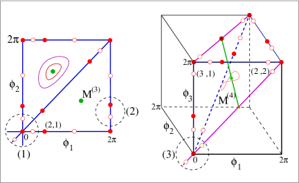
(a) (b)

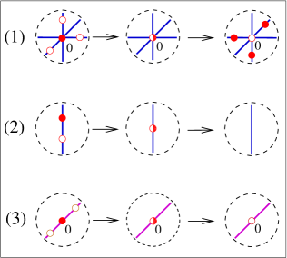
Figure 1: Illustration of bifurcations of steady states for $N=3$ (left panel in (a), the system in terms of phase differences $\varphi$ is two-dimensional), and $N=4$ (right panel in (a), the system in terms of phase differences $\varphi$ is three-dimensional). Panel (b) illustrates particular transitions in the selected regions of the phase space (see text for details).

Bifurcations of the completely synchronous state $\varphi_{j}=0$.

The origin of the system (6) is an equilibrium for any value of the function $\alpha(r,\beta)$. Consider the Jacobian matrix of this system at the point $\varphi_{j}=0$, $j=1,\cdots,N-1$. All eigenvalues of this matrix have the same value:

$$\lambda_{i}=-N\cos(\alpha(1,\beta)),\quad i=1,\cdots,N-1.$$

This means that the origin of the system changes its stability when $\alpha(1,\beta)=\pm\pi/2$. Also, as it was argued above, a bifurcation must be one-dimensional on each of the invariant lines with symmetry $S_{p}\times S_{N-p}$. This bifurcation can be either a transcritical or a pitchfork one. A pitchfork bifurcation can happen only in the case of an even number of oscillators and this bifurcation occurs along invariant lines with the symmetry $S_{N/2}\times S_{N/2}$ as it was shown in the work of Ashwin and Swift [21].

Thus, a typical bifurcation of the completely synchronous state is a transcritical bifurcation (see raw (1) in Fig. 1(b)). These bifurcations occur simultaneously on all invariant lines with the isotropies $S_{p}\times S_{N-p}$, $p\not=N/2$. Bifurcation parameters $\beta=(\beta_{1},\dots,\beta_{m})$ are defined from the expression $\alpha(1,\beta)=\pm\pi/2$. The steady state at the bifurcation point is a degenerate saddle (all eigenvalues of the linearized system are zero). $\sum_{j=1}^{[N+1]/2-1}C_{N}^{j}$ saddles, where [N] – integer part of $N$, meet together at the origin. The bifurcation changes stability of the origin along each of the one-dimensional directions.

A pitchfork bifurcation of the origin (see raw (3) in Fig. 1(b)) occurs simultaneously with the transcritical bifurcation, when the number of oscillators is even. Two saddles appear (disappear) from the origin (stable or unstable) and move in opposite directions along the lines which have $S_{N/2}\times S_{N/2}$ isotropy. In the case of an even $N$ these saddles are usually generators of trajectories (one–dimensional manifolds) which can be parts of heteroclinic cycles, under some additional conditions.

Clusters and their bifurcations.

To find all other steady states on the invariant lines with the symmetries $S_{p}\times S_{N-p}$ we should solve appropriate algebraic system (18) that satisfies (15) – this means that we need to solve one algebraic equation. Typically, steady states appear (or disappear) by pairs on each invariant lines for $\varphi_{j}\in(0,2\pi)$, $j=1,\cdots,N-1$, and this appearance (disappearance) corresponds to a saddle-node bifurcation (see raw (2) in Fig. 1(b)). A saddle-node bifurcation that occurs in the $(N-1)$-dimensional space (where our reduced system is considered) leads to the appearance of two new points, i.e. of two new two-cluster states. These two points have opposite stabilities along the one–dimensional manifold with isotropy $S_{p}\times S_{N-p}$, but the same stabilities transversal to these one-dimensional manifolds. In particular, one of these two newly appeared points can be a stable or an unstable node. A stable node on the one–dimensional invariant line corresponds to a two-cluster with symmetry $S_{p}\times S_{N-p}$.

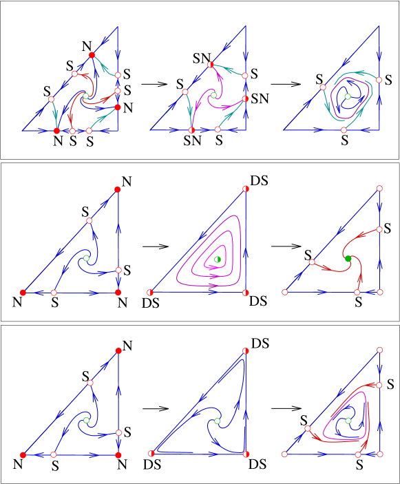
Figure 2: Illustration of bifurcations via heteroclinic cycles. Upper panel: HC appears via a saddle-node bifurcation and gives rise to a limit cycle. Middle panel: The case of Kuramoto-Sakaguchi, here at the bifurcation point a family of neutral cycles exist, while beyond it only a fully asynchronous steady state is stable. Bottom panel: HC appears via a transcritical bifurcation and gives rise to a limit cycle.

Heteroclinic and limit cycles.

Saddle steady states that appear in the transcritical and saddle-node bifurcations described above may have unstable manifolds that are connected to each other, thus constituting a heteroclinic cycle (see also a similar structure described in [22]). When the heteroclinic cycle disappears, a usual limit cycle may appear corresponding to a periodic non-synchronous regime in system (6). We illustrate two types of such a bifurcation in Fig. 2. In the upper panel we show an appearance of a limit cycle via a heteroclinic one, that appears at the saddle-node collision. Generation of a limit cycle by a saddle–node bifurcation via a heteroclinic cycle is a typical situation in the system (6). In the case of an even number of oscillators, saddle–node bifurcations on the invariant lines can give possibility to connect different one–dimensional manifolds of saddles (pairs of saddles) generated by pitchfork bifurcation from the origin. The bottom panel illustrates a heteroclinic cycle appearing at a transcritical bifurcation at the origin. Heteroclinic (or homoclinic) cycle consists of the origin point and loops of $S_{p}\times S_{N-p}$ invariant lines. The middle panel in Fig. 2 shows the same transcritical bifurcation in the Kuramoto-Sakaguchi model.

Another possibilities of a limit cycle to appear are an Andronov–Hopf bifurcation of the point of $\mathcal{M}$ (we will show this below), and a saddle–node bifurcation of two limit cycles. The existence of more complicated structures such as of a quasi–periodic torus or chaotic attractors is impossible for the system in phase differences (6). This follows from the Watanabe-Strogatz theory [16]. As it was shown in [16, 12], the system (4) can be reduced to a skew three–dimensional system where the equation for one variable fully depends on two other ones. Thus, the dynamics of the two “driving” variables can be at most periodic, and the full dynamics at most quasiperiodic. In the terms of variables we use here, the “driving” variables correspond to phase differences $\varphi_{k}$, their dynamics thus can be at most periodic. The full dynamics of phases $\theta_{k}$ includes one more integration and can be at most quasiperiodic.

Multistability.

If a saddle-node bifurcation generates a stable node while a stable node at the origin still exists, we obtain a bistability of a fully synchronized and two-cluster regimes. Note that depending on function $\alpha(r,\beta)$, we can obtain many stable nodes on the invariant lines, resulting in a multistability of synchronous and different two-cluster states.

One can also observe a coexistence of limit cycles appeared via different saddle–node bifurcations accompanied by heteroclinic cycles. Part of these cycles are stable but other ones are not.

Attractors.

As a result, one can observe the following types of possible stable regimes or their combinations in system (6):

1) Complete synchrony $\varphi_{j}=0$, $j=1,\cdots N$.

2) Two–cluster regime with symmetry $S_{p}\times S_{N-p}$.

3) Limit cycle.

4) Heteroclinic cycle.

5) Manifold $M^{(N)}$.

Stability of $\mathcal{M}$.

Consider the invariant set $\mathcal{M}$. This set is $(N-3)$–dimensional in $\mathbb{T}^{N-1}$ and consists of steady states of the system. To describe local bifurcations, we need to consider the property of Jacobin matrix

$$J=J(\varphi_{1},\dots,\varphi_{N-1},\alpha(r,\beta))=\frac{\partial(g_{1}(\varphi_{1},\dots,\varphi_{N-1},\alpha),\dots,g_{N-1}(\varphi_{1},\dots,\varphi_{N-1},\alpha))}{\partial(\varphi_{1},\dots,\varphi_{N-1})}$$

on the points of the manifold $\mathcal{M}$. We will show that $N-3$ eigenvalues of Jacobian vanish, so there is no any motion inside the manifold.

Lemma 3

Jacobian rank of the system (6) is:

$${\rm rank}(J)=\left\{\begin{array}[]{ll}1,&\mbox{for 2--clusters with symmetry}\ S_{N/2}\times S_{N/2},\\ 2,&\mbox{in other cases}.\end{array}\right.$$

Proof:  Jacobian matrix $J$ has the elements

$$J_{kk}=\frac{\partial g_{k}}{\partial\varphi_{k}}=-\left[\cos(\varphi_{k}-\alpha)-\frac{\partial\alpha}{\partial\varphi_{k}}\sum_{j=1}^{N-1}\cos(\varphi_{j}-\alpha)+\right.$$

$$+\left.\left(1+\frac{\partial\alpha}{\partial\varphi_{k}}\right)\left(\cos(\varphi_{k}+\alpha)+\sum_{j=1,j\not=k}^{N-1}\cos(\varphi_{k}-\varphi_{j}+\alpha)\right)\right],$$

$$J_{ki}=\frac{\partial g_{k}}{\partial\varphi_{i}}=-\left[\cos(\varphi_{i}-\alpha)-\cos(\varphi_{k}-\varphi_{i}+\alpha)-\frac{\partial\alpha}{\partial\varphi_{i}}\sum_{j=1}^{N-1}\cos(\varphi_{j}-\alpha)+\right.$$

$$+\left.\frac{\partial\alpha}{\partial\varphi_{i}}\left(\cos(\varphi_{k}+\alpha)+\sum_{j=1,j\not=k}^{N-1}\cos(\varphi_{k}-\varphi_{j}+\alpha)\right)\right],$$

Since we consider manifold $\mathcal{M}$, then using (8) and (5) we obtain

$$\cos\alpha+\sum_{j=1}^{N-1}\cos(\varphi_{j}-\alpha)=0$$

and

$$\cos(\varphi_{k}+\alpha)+\cos\alpha+\sum_{j=1,j\not=k}^{N-1}\cos(\varphi_{k}-\varphi_{j}+\alpha)=0.$$

Thus in this case elements of Jacobian matrix are

$$\frac{\partial g_{k}}{\partial\varphi_{j}}\bigg{|}_{M^{(N)}}=\cos(\varphi_{j}-\varphi_{k}-\alpha(0,\beta))-\cos(\varphi_{j}-\alpha(0,\beta)),\quad j,k=1,\dots,N-1.$$

Denote each column of matrix $J$ by $\overline{J}_{k}$, $k=1,\dots,N-1$. To prove that rank of matrix is not greater than two, we need to show that there exists the linear dependence between any three columns $\overline{J}_{i}$, $\overline{J}_{k}$, $\overline{J}_{l}$ of matrix $J$, i.e. there exist two scalar functions $\gamma_{j}$ and $\gamma_{k}$ such that

$$\gamma_{j}\overline{J}_{j}+\gamma_{k}\overline{J}_{k}=\overline{J}_{l}.$$

One can check that the last expression is satisfied with functions

$$\gamma_{j}=\frac{\sin(\varphi_{l}-\varphi_{k})}{\sin(\varphi_{j}-\varphi_{k})},\quad\gamma_{k}=\frac{\sin(\varphi_{l}-\varphi_{j})}{\sin(\varphi_{k}-\varphi_{j})},$$

when $\varphi_{j}\not=\varphi_{k}$. Thus ${\rm rank}(J)\leq 2$.

We can rewrite equation for vectors in the form

$$\sin(\varphi_{k}-\varphi_{l})\overline{J}_{j}+\sin(\varphi_{l}-\varphi_{j})\overline{J}_{k}+\sin(\varphi_{j}-\varphi_{k})\overline{J}_{l}=0.$$

All coefficients are not equal to zero in this expression when $\varphi_{i}\not=\varphi_{k}\not=\varphi_{l}$. Thus ${\rm rank}(J)$ is not less than two when the system has at least a three–cluster regime. Then ${\rm rank}(J)=2$ for three–or–more cluster regimes.

In the case of even number of oscillators $N=2p$ the system can have two–cluster states with symmetry $S_{N/2}\times S_{N/2}$ that belong to invariant manifold ${\cal M}$. This means that in the last equation one coefficient is equal to zero that implies ${\rm rank}(J)=1$. The lemma is proved.

The lemma shows that the Jacobian has $N-3$ eigenvalues equal to zero at the points of manifold $\mathcal{M}$. However, as it was shown, the rank of the Jacobian depends on values of the variables (i.e. on the coordinates of points on the manifold). Thus, to find the eigenvalues of $J$ we need to consider not only $2\times 2$ minor of Jacobian matrix but the whole matrix. Each of the eigenvalues is a function of $N-3$ variables in the points of the manifold. Let us express the last two variables $\varphi_{N-2}$ and $\varphi_{N-1}$ as the functions of the variables $\varphi_{1},\dots,\varphi_{N-3}$ using expressions of real and imaginary parts of (8). Then we obtain:

$$\varphi_{N-2}=\arctan\left(\frac{f_{2}}{f_{1}}\right)-\frac{1}{2}\arccos\left(\frac{f_{1}^{2}+f_{2}^{2}}{2}-1\right)+\frac{\pi}{2}(1-{\rm sign}(f_{1})),$$

$$\varphi_{N-1}=\arctan\left(\frac{f_{2}}{f_{1}}\right)+\frac{1}{2}\arccos\left(\frac{f_{1}^{2}+f_{2}^{2}}{2}-1\right)+\frac{\pi}{2}(1-{\rm sign}(f_{1})),$$

where

$$f_{1}(\varphi_{1},\dots,\varphi_{N-3})=-1-\sum_{j=1}^{N-3}\cos\varphi_{j},\quad f_{2}(\varphi_{1},\dots,\varphi_{N-3})=-\sum_{j=1}^{N-3}\sin\varphi_{j}.$$

In the case of a uniform distribution of oscillators on the circle (splay state according to terminology used for Kuramoto model [16]), that is when

$$\varphi_{1}=\frac{2\pi}{N},\quad\varphi_{j}=j\varphi_{1},\quad j=2,\dots,N-1,$$

the eigenvalues of the Jacobian are

$$\lambda_{N-2,N-1}=\frac{N}{2}(\cos\alpha\pm i\sin\alpha).$$

In general case the eigenvalues are

$$\lambda_{N-2,N-1}(\varphi_{1},\dots,\varphi_{N-3})=\frac{N}{2}\left(\cos\alpha\pm\sqrt{\cos^{2}\alpha-h^{2}(\varphi_{1},\dots,\varphi_{N-3})}\right),$$

where $|h(\varphi_{1},\dots,\varphi_{N-3})|\leq 1$ is some enough complicate smooth function. Therefore, we obtain an Andronov–Hopf bifurcation when $\alpha=\pm\pi/2$. This bifurcation happens simultaneously in each point of manifold $\mathcal{M}$ except for the points with isotropy $S_{N/2}\times S_{N/2}$ where function $h(\varphi_{1},\dots,\varphi_{N-3})=0$.

In the case of three coupled phase oscillators, the zero–dimensional manifold $\mathcal{M}^{(3)}$ consists of two points $(2\pi/3,4\pi/3)$ and $(4\pi/3,2\pi/3)$. At the point of an Andronov–Hopf bifurcation each of these two points changes its stability and generates supercritically (or destroys subcritically) a limit cycle. With a further variation of a parameter, this limit cycle can grow in amplitude and disappear, either in a saddle-node/heteroclinic bifurcation, or via a saddle-node bifurcation of two limit cycles.

More nontrivial situations can happen in the case of four globally coupled oscillators. Invariant manifold $\mathcal{M}^{(4)}$ in this case consists of six straight lines. Coordinates of such lines are $(\varphi_{j},\pi,\varphi_{j}+\pi)$ up to permutations. Invariant manifold has $Z_{2}$ isotropy. The function $h(\varphi_{j})=\sin\varphi_{j}$ appears in the expressions for the eigenvalues of the Jacobian matrix. An Andronov–Hopf bifurcation happens simultaneously in each of the manifold points. Thus, we obtain a two dimensional surface that consists of limit cycles. Noteworthy, the bifurcation differs from a Neimark–Sacker bifurcation. Each of this cycles is attractive (repulsive) only inside the surfaces described by Watanabe–Strogatz theory [16], in other direction it is neutral. Possible way of this two-dimensional surface to disappear a is saddle-node heteroclinic bifurcation on invariant lines described. A two–dimension set of heteroclinic cycles occurs at the point of bifurcation (such a set was shown in figure 10 in [22]).

Another possibility is disappearance (appearance) of two limit cycles in a saddle–node bifurcation of cycles. We can note that such a bifurcation happens for each pair of limit cycles which belong to different two–dimensional sets of cycles. Such a bifurcation happens also inside the Watanabe–Strogatz surfaces. Thus we obtain a saddle–node bifurcation of two–dimensional surfaces, one of them is stable and other is unstable.

4 Nonlinearly coupled oscillators with quadratic phase nonlinearity

As an example of application of general picture outlined above we consider the model (4) with particular dependence of the phase shift on the amplitude of the mean field [12]:

$$\alpha=\alpha(r,\beta)=\beta_{1}+\beta_{2}r^{2}.$$ (20)

Here the two–dimensional space of parameters $(\beta_{1},\beta_{2})$ is a cylinder $\mathbb{R}\times\mathbb{T}\supset(\beta_{2},\beta_{1})$, because the r.h.s. of the equations are $2\pi$–periodic with respect to $\beta_{1}$. The oddness of the r.h.s. of the system implies the symmetry of the parameter plane $(\beta_{1},\beta_{2})\to(-\beta_{1},-\beta_{2})$.

According to the consideration above, two types of bifurcation happen when

$$\cos(\alpha)=\cos(\beta_{1}+\beta_{2}r^{2})=0.$$

One possible bifurcation is an Andronov–Hopf bifurcation (AH) on the invariant manifold $\mathcal{M}$. Since $r=0$ on the manifold, then we obtain two straight bifurcation lines

$$\beta_{1}=\pi/2\quad\mbox{and}\quad\beta_{1}=3\pi/2$$ (21)

on the parameter cylinder. The line $\beta_{1}=\pi/2$ corresponds to a supercritical Andronov–Hopf bifurcation and the line $\beta_{1}=3\pi/2$ corresponds to a subcritical one. Manifold $\mathcal{M}$ is stable if $\beta_{1}\in(\pi/2,\ 3\pi/2)$ and it is unstable if $\beta_{1}\in[0,\pi/2)\cup(3\pi/2,2\pi)$.

Another possible bifurcation is a transcritical bifurcation (TC) at the origin ($\varphi_{j}=0$, $j=1,\dots,N-1$) along each of the invariant lines with the symmetry $S_{p}\times S_{N-p}$, $p=1,\dots,N-1$. A pitchfork bifurcation (PF) at the origin occurs, simultaneously with the transcritical one, along the invariant lines with the symmetry $S_{N/2}\times S_{N/2}$ for the system with even number of oscillators. At this bifurcation point the origin is a degenerate saddle with $N-1$ zero eigenvalues. The origin point of the system corresponds to full synchronization state where order parameter $r=1$. Therefore, straight lines

$$\beta_{1}+\beta_{2}=\pi/2+\pi m,\quad m\in\mathbb{Z},$$ (22)

correspond to the transcritical (TC) or to the transcritical–pitchfork (TC/PF) bifurcations in the parametric space. The origin (i.e. the regime of full synchrony) is stable when $\beta_{1}+\beta_{2}\in(-\pi/2+2\pi m,\ \pi/2+2\pi m)$, $m\in\mathbb{Z}$, and it is unstable when $\beta_{1}+\beta_{2}\in(\pi/2+2\pi m,\ 3\pi/2+2\pi m)$.

These two types of bifurcation are independent of the number of oscillators, so the grids of straight bifurcation lines (21,22) are present at any bifurcation diagram model (20) (Figs. 3, 7). Other bifurcations of the fixed points occur only on invariant lines (15) and they all are of the saddle–node type. The expressions for the order parameter on the invariant lines (15) are

$$r^{2}=r^{2}(p,N-p)=\frac{1}{N^{2}}(2p(N-p)\cos(\varphi_{k})+(N-1)^{2}-2(p-1)(N-p-1)+1),$$

where $\varphi_{k}$, $k=1,\dots,p$, is a variable that changes along invariant lines with $S_{p}\times S_{N-p}$ isotropy. To find the coordinates of the steady states we need to solve equation (19) with this expression for the order parameter. This expression simplyfies in the case of even number oscillators to

$$r^{2}(p,p)=\frac{1}{2}(\cos(\varphi_{k})+1),\quad k=1,\dots,p\;,$$

and is independent of the number of oscillators. Thus, it describes appearance (disappearance) of two points on the invariant line with symmetry $S_{N/2}\times S_{N/2}$ after each pitchfork bifurcation at the origin. The coordinates of these points (which are saddles) on the invariant lines are then

$$\varphi_{k}=\pm\arccos\left(\frac{1}{\beta_{2}}(\pi(1+2m)-2\beta_{1}-\beta_{2})\right),\quad m\in\mathbb{Z}.$$

These symmetric points are important because they are the basis for heteroclinic cycles in cases of even number of oscillators.

For any number of oscillators, together with the grid of the straight lines describing Andronov–Hopf and transcritical bifurcations (21,22), there are a lot of bifurcation lines that correspond to saddle–node bifurcations (SN) on invariant lines. Some of these lines correspond to heteroclinic bifurcations (HC or HC(SN)), provided some additional conditions are satisfied. At these saddle–node/heteroclinic bifurcations limit cycles appear. Let us fix some parameter value $\beta_{1}\not=\pm\pi/2$ and increase parameter $\beta_{2}$. Then new and new saddle–node bifurcations occur on the invariant lines, steady states appear at these bifurcations in such a way that their stability alternate along this line. Stability of appearing heteroclinic cycles also alternates with increasing of the parameter $\beta_{2}$. Thus, stabilities of limit cycles that move inside each invariant region after such a bifurcation also alternate. The period and the amplitude of each of the limit cycles decrease when parameter $\beta_{2}$ increases, but no bifurcation of small limit cycle can happen because we demanded that $\beta_{1}$ was not equal to $\pm\pi/2$ where such a bifurcation only could occur.

The number of the hyperbolic steady states increases with increasing of parameter $\beta_{2}$. These steady states tend to concentrate near the center part of the invariant lines. A saddle–node/heteroclinic bifurcation on the line with symmetry $S_{1}\times S_{N-1}$ usually occurs close to this central region, where the coordinate $\varphi$ of the saddle–node point is close to $\pi$. Thus, we can approximately calculate that such bifurcation occurs at

$$\beta_{2}\approx\frac{N^{2}}{(N-2)^{2}}(\pi m-\beta_{1}),\quad m\in\mathbb{Z}.$$

The lines of a saddle–node/heteroclinic bifurcation alternates on the bifurcation cylinder. Each heteroclinic cycle generates a limit cycle (or a set of limit cycles for 4 and more oscillators) with the same stability. The period and the size of each cycle decrease with increasing of parameter $\beta_{2}$. Stable and unstable limit cycles enwrap each other inside invariant region, and alternate. A saddle–node bifurcation of limit cycles is impossible for the system considered because of monotonic increase of cycles sizes (it would be, however, possible for more complex than (20) dependencies $\alpha(r)$, e.g. for $\alpha=\beta_{1}+\beta_{2}r^{2}+\beta_{3}r^{4}$).

Noteworthy, the first saddle–node bifurcation in the system usually happens when $\beta_{2}<\pi/2-\beta_{1}$, and this bifurcation can generate a stable node. Then we obtain multistability of the fully synchronous state (the origin where $r=1$) and the stable two–cluster states. If the first transcritical bifurcation (when $\beta_{2}>\pi/2-\beta_{1}$) doesn’t produce a stable heteroclinic cycles, then the two–cluster states are the only attractors in the system. The stable nodes accumulate on the invariant line with increasing $\beta_{2}$, thus we obtain a multistability of two–cluster states when $\beta_{2}$ is large enough. The appearance of stable limit cycles after saddle–node/heteroclinic bifurcation eliminates one stable node (on each invariant line with the same symmetry). However, since a heteroclinic bifurcation happens more rarely than simple saddle–node bifurcations of two points, then the coexistence of a stable limit cycle with two–cluster states is typical for the system. Therefore, we can obtain multistability of all possible attractors in the system: full synchronous state, two–cluster state (with different order parameters), limit cycle of phase differences, heteroclinic cycle, and invariant manifold $\mathcal{M}$.

4.1 Three interacting oscillators

For three oscillators interacting according to phase shift (20), the bifurcation diagram is depicted in Fig. 3. The corresponding bifurcations have been already illustrated in Figs. 1,2 above. According to this bifurcation diagram, we show in Fig. 4 a schematic dependence of the synchronization states in the system as parameter $\beta_{2}$ changes while $\beta_{1}=0$. One can see that the basic transition in terms of phase differences is: Full synchrony $\to$ two-cluster state $\to$ periodic oscillations. The first transition is with hysteresis (i.e. in some small region of parameters full synchrony and two-cluster state coexist), and the second transition is via heteroclinic connection. On the diagram Fig. 3 several codimension-2 points are marked, we will discuss them in the next subsection.

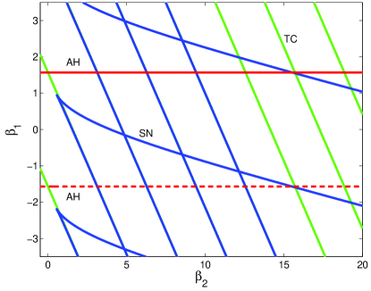
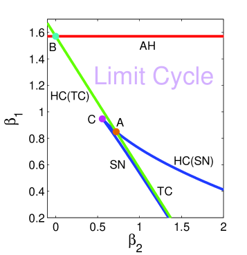
Figure 3: Bifurcation diagram for $N=3$ oscillators in the $(\beta_{2},\beta_{1})$ parametric plane (cf. Fig. 1(a)). Right panel is an enlargement of the central part of the left one. TC — transcritical bifurcation (see Fig. 1(b)(1)), SN — saddle–node bifurcation (see Fig. 1(b)(2)), AH — supercritical Andronov–Hopf bifurcation (see Fig. 1(b)(4)), HC(SN), HC(TC) heteroclinic bifurcations (see Fig. 2). Points A, B and C are codimension–two bifurcation points. The region where a stable limit cycle exists (right panel) is surrounded by a supercritical AH bifurcation line and two lines of heteroclinic bifurcations of different types.

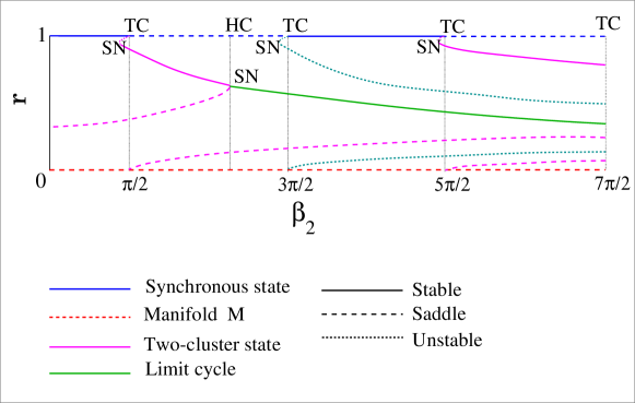
Figure 4: Schematic bifurcation diagram for the $(\beta_{2},r)$ parametric plane and the case $\alpha=\beta_{2}r^{2}$. TC — transcritical bifurcation, HC — heteroclinic cycle (bifurcation), SN — saddle–node bifurcation.

4.2 Four and more coupled oscillators

In the Figures 5 and 6 we show schematically a saddle–node/heteroclinic bifurcation for the case $N=4$. An unstable heteroclinic cycle (Figure 5) consists of ten fixed points and ten 1–dimensional invariant manifolds that connect these points. Four saddle–node bifurcations happen simultaneously on four $S_{1}\times S_{3}$ invariant lines. This heteroclinic cycle includes also two saddles $S^{\prime}$ that belong to $S_{2}\times S_{2}$ invariant line. Thus, the system of four oscillators, that moves along this heteroclinic cycle, shows temporary switches between $1+3$ and $2+2$ clustering. This unstable heteroclinic cycle is robust and it will exist also beyond the saddle-node bifurcation; however it will consist of two lines connecting $S^{\prime}$ only, like the stable cycle depicted in the figure. This stable heteroclinic cycle is shown inside the unstable one. It consists of two saddles $S^{\prime\prime}$ and two connecting lines $\Gamma_{1}$, $\Gamma_{2}$. The stable heteroclinic cycle appears at a saddle–node bifurcation on the invariant line in the same way as the unstable one, only for a smaller value of parameter $\beta_{2}$. The next heteroclinic bifurcation will occur after merging of stable node $N^{+}$ and saddle $S$ and it will produce causes stable heteroclinic cycle.

Figure 6 shows an appearance of a 2–dimensional sets of stable limit cycles inside one invariant region. Four pairs of saddles $S$ and stable nodes $N$ (Fig. 6 a) ) collide and create 2–dimensional sets of heteroclinic cycles (Fig. 6 b) ). Beyond the bifurcation, when saddle–node points $SN$ disappear, two heteroclinic cycles appear, with 2–dimensional sets of limit cycles between them (Fig. 6 c) ). The set of limit cycles surrounds the 1–dimensional invariant set $\mathcal{M}$. This set of limit cycles shrinks as parameter $\beta_{2}$ increases, but it never reaches manifold $\mathcal{M}$.

The heteroclinic cycles presented in Fig. 5 lie on invariant surfaces and correspond to switches between the cluster states. They are borders of sets of limit cycles that exist inside the bulk of the phase space (that is bounded by the invariant lines and surfaces), and enwrap the manifold $\mathcal{M}$. To an unstable HC corresponds a cylindrical set of unstable limit cycles, and to a stable HC corresponds a cylindrical set of stable limit cycles. In this way the structure of heteroclinic cycles determines the overall structure of the trajectories also outside of invariant manifolds.

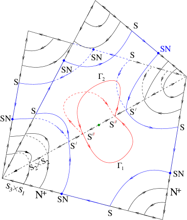
Figure 5: Schematic phase portrait for $N=4$ coupled oscillators, showing only invariant lines corresponding to cluster states $1+3$ and $2+2$, and planes connecting them. We illustrate a coexistence of two types of heteroclinic cycles. One unstable HC (blue) is shown at the bifurcation point, another stable HC (red) is beyond its bifurcation.

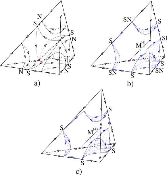
Figure 6: Schematic diagrams of the saddle–node/heteroclinic bifurcation for 4 globally coupled oscillators. a) – prior bifurcation, b) – at the bifurcation point, c) beyond bifurcation.

The bifurcation analysis of higher–dimensional cases (for $N\geq 5$) shows similar results. The bifurcation diagram consists of three types of lines: a straight line of an Andronov–Hopf bifurcation, a straight line of a transcritical bifurcation, and lines of saddle–node bifurcations on invariant lines with the symmetry $S_{p}\times S_{N-p}$, $p=1,\dots,N-1$. All the saddle–node bifurcation lines have similar “tongue-like” form. The “tongue” is formed by two border lines: one lies left of the straight line of a transcritical bifurcation and approaches this line asymptotically with increasing of parameter $\beta_{2}$, the second border line crosses the TC–lines. The saddle–node bifurcation generates a sink and source only on the invariant line with symmetry $S_{1}\times S_{N-1}$, while on other invariant lines with the symmetry $S_{p}\times S_{N-p}$, $p\not=1$ a pair of saddles appears. Therefore, there exist only $1\times(N-1)$ stable clusters. Furthermore, heteroclinic cycles and stable limit cycles appear at a saddle–node bifurcation with $S_{1}\times S_{N-1}$ symmetry only (the corresponding bifurcation lines are drawn with blue in Fig. 7).

Let us discuss the codimension-two points marked in Fig. 3. At point $C$ two borders of the saddle-node tongue meet. Only one stable state is involved in both saddle-node bifurcations (say, on the left line states $1$ and $2$ are created, while on the right line state $2$ annihilates with state $3$), at the codimension-two point $C$ all three involved steady states meet. At another codimension-two point $A$ the type of the saddle-node bifurcation changes. On one side (left to the point $A$) no heteroclinic cycle appears at the saddle-node, while right to point $A$ the transition can be saddle-node/heteroclinic, provided $-\pi/2<\beta_{1}(A)<\pi/2$ and the line has symmetry $S_{1}\times S_{N-1}$. We have checked that the latter condition holds for $N=3,\ldots,8$ only and for $N\geq 9$ one has $\beta_{1}(A)<-\pi/2$. Thus, for $N\geq 9$ there is no saddle-node/heteroclinic transition. Finally, the point $B$ on the bifurcation diagram Fig. 3 corresponds to a degenerate situation depicted in the middle panel of Fig. 2.

We show bifurcation diagrams on the planes $(\beta_{1},\beta_{2})$ for four and five coupled oscillators in Fig. 7. The structure of these diagrams is basically the same as for three oscillators Fig. 3, but with some quantitative changes. To clarify these changes we compare in Fig. 8 the basic saddle-node “tongues” for $N=3,\ldots,7$. One can see that with increase of $N$ the tip shifts down and for a fixed $\beta_{1}\approx 0$ the saddle-node bifurcation can be observed for a small number of oscillators only. Thus, for a fixed $\beta_{1}\approx 0$ the loss of full synchrony with increase of $\beta_{2}$ occurs as direct transition from full synchrony to periodic oscillations via a transcritical bifurcation (bottom raw in Fig. 2), and not via clustered states.

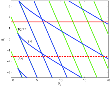
(a) (b)

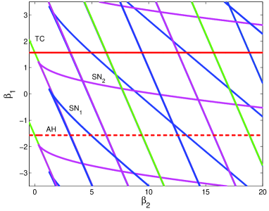
Figure 7: Bifurcation diagrams for (a) $N=4$ and (b) $N=5$ oscillators in the $(\beta_{2},\beta_{1})$ parametric plane. In (b): $SN_{1}$ — the line of saddle–node bifurcation on $S_{4}\times S_{1}$ invariant line, $SN_{2}$ — the same with the $S_{3}\times S_{2}$ invariant line.

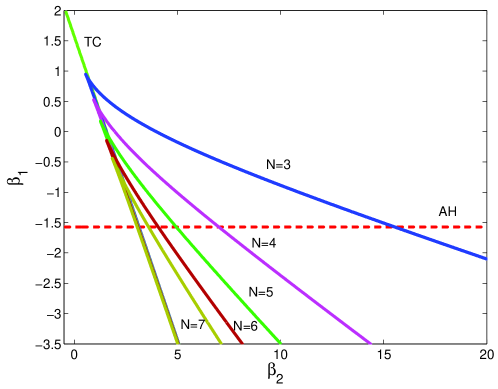
Figure 8: The comparative diagram of saddle–node bifurcation lines on the $(\beta_{2},\beta_{1})$ parametric plane for the cases 3, 4, 5, 6, and 7 oscillators. The tip of the “tongues” shifts down as $N$ grows, and for $N\geq 9$ is below thee line of Andronov-Hopf bifurcation $\beta_{1}=-\pi/2$.

5 Conclusion

In this paper we have performed a detailed bifurcation analysis of the nonlinear generalization of the Sakaguchi-Kuramoto model of globally coupled phase oscillators. The main novelty in addition to the consideration in the framework of WS theory [12] is the characterization of cluster states that in terms of phase differences appear (via a transcritical, a pitchfork, or a saddle-node bifurcation) as steady states on invariant lines of the corresponding cluster configurations. At saddle-node bifurcations these steady states disappear via heteroclinic cycles. Remarkably, heteroclinic cycles in this model are not destroyed but remain to exist (for other examples of heteroclinic cycles in ensembles of identical phase oscillators see [23, 24, 20]). This is related to the partial integrability of the system resulting from the WS theory. According to WS, because the equations have $N-3$ constants of motion, periodic orbits form the families of corresponding dimensions, the heteroclinic cycles form the limiting cases of these families, describing cycles that include nearly-clustered states.

The analysis performed in this paper complemented the conclusion on the transition from full to partial synchrony in nonlinearly coupled oscillator ensembles, made in [12]. We have demonstrated that for small ensembles the transition is of the type “full synchrony” $\to$ “cluster state” $\to$ “periodic/quasiperiodic partially synchronous state” occurs, while for a large number of oscillators a direct transition “full synchrony” $\to$ “periodic/quasiperiodic partially synchronous state” is typical.

Acknowledgement O.B. thanks DFG (Project “Collective phenomena and multistability in networks of dynamical systems”) for support. We thank M. Rosenblum, P. Ashwin, and M. Wolfrum for useful discussions.

References

- [1] K. Wiesenfeld and J. W. Swift. Averaged equations for Josephson junction series arrays. Phys. Rev. E, 51(2):1020–1025, 1995.
- [2] A. F. Glova. Phase locking of optically coupled lasers. Quantum Electronics, 33(4):283–306, 2003.
- [3] I.Z. Kiss, Y. Zhai, and J.L. Hudson. Emerging coherence in a population of chemical oscillators. Science, 296:1676–1678, 2002.
- [4] D. Golomb, D. Hansel, and G. Mato. Mechanisms of synchrony of neural activity in large networks. In F. Moss and S. Gielen, editors, Neuro-informatics and Neural Modeling, volume 4 of Handbook of Biological Physics, pages 887–968. Elsevier, Amsterdam, 2001.
- [5] Y. Kuramoto. Self-entrainment of a population of coupled nonlinear oscillators. In H. Araki, editor, International Symposium on Mathematical Problems in Theoretical Physics, page 420, New York, 1975. Springer Lecture Notes Phys., v. 39.
- [6] Y. Kuramoto. Chemical Oscillations, Waves and Turbulence. Springer, Berlin, 1984.
- [7] H. Daido. Onset of cooperative entrainment in limit-cycle oscillators with uniform all-to-all interactions: Bifurcation of the order function. Physica D, 91:24–66, 1996.
- [8] H. Sakaguchi and Y. Kuramoto. A soluble active rotator model showing phase transition via mutual entrainment. Prog. Theor. Phys., 76(3):576–581, 1986.
- [9] A. Pikovsky, M. Rosenblum, and J. Kurths. Synchronization. A Universal Concept in Nonlinear Sciences. Cambridge University Press, Cambridge, 2001.
- [10] S. H. Strogatz. From Kuramoto to Crawford: Exploring the onset of synchronization in populations of coupled oscillators. Physica D, 143(1-4):1–20, 2000.
- [11] M. Rosenblum and A. Pikovsky. Self-organized quasiperiodicity in oscillator ensembles with global nonlinear coupling. Phys. Rev. Lett., 98:064101, 2007.
- [12] A. Pikovsky and M. Rosenblum. Self-organized partially synchronous dynamics in populations of nonlinearly coupled oscillators. Physica D, 238(1):27–37, 2009.
- [13] G. Filatrella, N. F. Pedersen, and K. Wiesenfeld. Generalized coupling in the Kuramoto model. Phys. Rev. E, 75:017201, 2007.
- [14] F. Giannuzzi, D. Marinazzo, G. Nardulli, M. Pellicoro, and S. Stramaglia. Phase diagram of a generalized Winfree model. Phys. Rev. E, 75:051104, 2007.
- [15] S. Watanabe and S. H. Strogatz. Integrability of a globally coupled oscillator array. Phys. Rev. Lett., 70(16):2391–2394, 1993.
- [16] S. Watanabe and S. H. Strogatz. Constants of motion for superconducting Josephson arrays. Physica D, 74:197–253, 1994.
- [17] A. Pikovsky and M. Rosenblum. Dynamics of heterogeneous oscillator ensembles in terms of collective variables. Physica D, 2011.
- [18] V. Afraimovich, P. Ashwin, and V. Kirk, Editors. A focus issue on Robust Heteroclinic and Switching Dynamics. Dynamical Systems, vol. 25, n. 3, 2010.
- [19] M. Golubitsky and I. Stewart. The Symmetry Perspective. From Equilibrium to Chaos in Phase Space and Physical Space. Birkhäuser, Basel, 2002.
- [20] P. Ashwin, O. Burylko, Y. Maistrenko, and O. Popovych. Extreme sensitivity to detuning for globally coupled phase oscillators. Phys. Rev. Lett., 96(5):054102, 2006.
- [21] P. Ashwin and J. W. Swift. The dynamics of n weakly coupled identical oscillators. J. Nonlinear Sci., 2:69–108, 1992.
- [22] P. Ashwin, O. Burylko, and Y. Maistrenko. Bifurcation to heteroclinic cycles and sensitivity in three and four coupled phase oscillators. Physica D, 237:454–466, 2008.
- [23] D. Hansel, G. Mato, and C. Meunier. Clustering and slow switching in globally coupled phase oscillators. Phys. Rev. E., 48(5):3470–3477, 1993.
- [24] H. Kori and Y. Kuramoto. Slow switching in globally coupled oscillators: robustness and occurrence through delayed coupling. Phys. Rev. E, 63:046214, 2001.