A precise response function for the magnetic component of Gravitational Waves in Scalar-Tensor Gravity

Abstract

The important issue of the magnetic component of gravitational waves (GWs) has been considered in various papers in the literature. From such analyses, it resulted that such a magnetic component becomes particularly important in the high frequency portion of the frequency range of ground based interferometers for GWs which arises from standard General Theory of Relativity (GTR).

Recently, such a magnetic component has been extended to GWs arising from Scalar-Tensor Gravity (STG) too. After a review of some important issues on GWs in STG, in this paper we re-analyse the magnetic component in the framework of STG from a different point of view, by correcting an error in a previous paper and by releasing a more precise response function. In this way, we also show that if one neglects the magnetic contribution considering only the low-frequency approximation of the electric contribution, an important part of the signal could be, in principle, lost. The determination of a more precise response function for the magnetic contribution is important also in the framework of the possibility to distinguish other gravitational theories from GTR.

At the end of the paper an expansion of the main results is also shown in order to recall the presence of the magnetic component in GRT too.

International Institute for Theoretical Physics and Mathematics Einstein-Galilei, Via Santa Gonda, 14 - 59100 PRATO, Italy

E-mail addresses: cordac.galilei@gmail.com

Keywords: scalar gravitational waves; interferometers; magnetic components.

PACS numbers: 04.80.Nn, 04.80.-y, 04.25.Nx

1 Introduction

The data analysis of interferometric GWs detectors has nowadays been started, and the scientific community hopes in a first direct detection of GWs in next years; for the current status of GWs interferometers see Ref. [1]. In such a way, the indirect evidence of the existence of GWs by Hulse and Taylor [2], Nobel Prize winners, will be confirmed. Detectors for GWs will be important for a better knowledge of the Universe and also because the interferometric GWs detection will be the definitive test for GTR or, alternatively, a strong endorsement for Extended Theories of Gravity (ETG) [3]. On the other hand, the discovery of GW emission by the compact binary system composed by two Neutron Stars PSR1913+16 [2] has been, for physicists working in this field, the ultimate thrust allowing to reach the extremely sophisticated technology needed for investigating in this field of research [1]. GWs are a consequence of Einstein’s GTR [4], which presuppose GWs to be ripples in the space-time curvature travelling at light speed [5, 6]. In GTR only asymmetric astrophysics sources can emit GWs [7]. The most efficient are coalescing binaries systems at frequencies around 1 KHz [1], while a single rotating pulsar can rely only on spherical asymmetries, usually very small [1, 7]. Its spin frequency often lie in the hectohertz “sweet spot” of current detectors, i.e. at order hundreds Hz [49]. Supernovae could have relevant asymmetries, being potential sources [7]. It is generally agreed that the frequency of GW emission from the birth of stellar mass collapsed objects is in the range 50Hz to a few KHz [50]. The most important cosmological source of GWs is, in principle, the so-called stochastic background of GWs which, together with the Cosmic Background Radiation (CBR), would carry, if detected, a huge amount of information on the early stages of the Universe evolution [8, 9, 10, 11]. The existence of a relic stochastic background of GWs is a consequence of generals assumptions. Essentially it derives from a mixing between basic principles of classical theories of gravity and of quantum field theory [8, 9, 10, 11]. The strong variations of the gravitational field in the early universe amplify the zero-point quantum oscillations and produce relic GWs. It is well known that the detection of relic GWs is the only way to learn about the evolution of the very early universe, up to the bounds of the Planck epoch and the initial singularity [8, 11]. It is very important to stress the unavoidable and fundamental character of this mechanism. The model derives from the inflationary scenario for the early universe [12], which is consistent with the WMAP data on the CBR (in particular exponential inflation and spectral index $\approx$ 1 [13]). Inflationary models are cosmological models in which the Universe undergoes a brief phase of a very rapid expansion in early times [12]. In this tapestry the expansion could be power-law or exponential in time. Such models provide solutions to the horizon and flatness problems and contain a mechanism which creates perturbations in all fields [12]. Important for our case is that this mechanism also provides a distinctive spectrum of relic GWs [8, 10, 11]. The GWs perturbations arise from the uncertainty principle and the spectrum of relic GWs is generated from the adiabatically-amplified zero-point fluctuations [8, 9, 10, 11]. In standard cosmology such a spectrum is flat along the frequency range $10^{-16}\leq f\leq 10^{8}\mbox{ }Hz$ [51].

Regarding the potential GW detection, let us recall some historical notes. In 1957, F. A. E. Pirani, who was a member of the Bondi’s research group, proposed the geodesic deviation equation as a tool for designing a practical GW detector [14]. In 1959, Joseph Weber [15], First Award Winner at the 1959 Gravity Research Foundation Competition, studied a detector that, in principle, might be able to measure displacements smaller than the size of the nucleus. He developed an experiment using a large suspended bar of aluminium, with a high resonant Q at a frequency of about 1 kHz. Then, in 1960, he tried to test the general relativistic prediction of GWs from strong gravity collisions [16] and, in 1969, he claimed evidence for observation of GWs (based on coincident signals) from two bars separated by 1000 km [17]. He also proposed the idea of doing an experiment to detect GWs by using laser interferometers [17]. In fact, all the modern detectors can be considered like being originated from early Weber’s ideas [1, 7, 18]. At the present time, in the world there are five cryogenic bar detectors which have been built to work at very low temperatures ($<4K$): Explorer at CERN, Nautilus at Frascati INFN National Laboratory, Auriga at Legnaro National Laboratory, Allegro at Luisiana State University and Niobe in Perth [7, 18]. Instrumental details can be found in [18] and references within. Spherical detectors are the Mario Schenberg, which has been built in San Paolo (Brazil) and the MiniGRAIL, which has been built at the Kamerlingh Onnes Laboratory of Leiden University, see [7, 18, 19] and references within. Spherical detectors are important for the potential detection of the scalar component of GWs that is admitted in ETG [19]. In the case of interferometric detectors, free falling masses are interferometer mirrors which can be separated by kilometres (3km for Virgo, 4km for LIGO) [1, 7, 18]. In this way, GW tidal force is, in principle, several order of magnitude larger than in bar detectors. Interferometers have very large bandwidth ($10-10000\mbox{ }Hz$) because mirrors are suspended to pendulums having resonance in the Hz region. Thus, above such a resonance frequency, mirrors work, in a good approximation, like freely falling masses in the horizontal plane [1, 7, 18].

Now, let us recall the importance to distinguish the gravitational theories by using the observation of GWs [20]. Motivations to extend GTR arise from the fact that even though Einstein’s theory [4] has achieved great success (see for example the opinion of Landau, who said that GTR is, together with Quantum Field Theory, the best scientific theory of all [21]) and passed a lot of experimental tests [22] it has also showed some shortcomings and flaws which today prompt theorists to ask if it is the definitive theory of gravity [3]. Differently from other field theories like the electromagnetic theory, GTR is very difficult to quantize [23]. This fact rules out the possibility of treating gravitation like other quantum theories, and precludes the unification of gravity with other interactions. At the present time, it is not possible to realize a consistent Quantum Gravity Theory which leads to the unification of gravitation with the other forces [23]. On the other hand, one can define ETG, those semi-classical theories where the Lagrangian is modified, with respect to the standard Einstein–Hilbert gravitational Lagrangian, adding high order terms to the curvature invariants (terms like $R^{2}$, $R^{ab}R_{ab}$, $R^{abcd}R_{abcd}$, $R\Box R$, $R\Box^{k}R$, in the sense of the so-called $f(R)$ theories, see the recent review [24]) and/or terms with scalar fields non-minimally coupled to geometry (terms like $\phi^{2}R$ in the sense of the so-called Scalar-Tensor Theories [25], i.e. generalizations of the Jordan-Fierz-Brans-Dicke theory of gravitation [26, 27, 28]). In general, one has to emphasize that terms like those are present in all the approaches to performing the unification between gravity and other interactions. In addition, from a cosmological point of view, such modifications of GTR produce inflationary frameworks, which are very important as they solve a lot of problems of the Standard Universe Model [12]. Note that we are not saying that GTR is wrong. It is well known that, even in the context of extended theories, GTR remains the most important part of the structure [3, 24]. We are only trying to understand if weak modifications on such a structure could be needed to solve some theoretical and observing problems.

In the general context of cosmological evidences, there are other considerations which suggest an extension of GTR. As a matter of fact, the accelerated expansion of the Universe, which is today observed, shows that the cosmological dynamic is dominated by the so-called dark energy, which gives a large negative pressure. This is the standard picture, in which such a new ingredient is considered as a source of the right side of the field equations. It should be some form of unclustered non-zero vacuum energy which, together with the clustered dark matter, drives the global dynamics. This is the so-called “concordance model” ($\Lambda CDM$), which gives, in agreement with the CMBR, LSS and SNeIa data, a good tapestry of today’s observed Universe, but presents several shortcomings, such as the well-known “coincidence” and “cosmological constant” problems [29]. An alternative approach is to change the left side of the field equations, seeing if observed cosmic dynamics can be achieved by extending GTR [3]. In this different context, we are not required to find candidates for dark energy and dark matter, which till now have not been found, but only the “observed” ingredients, which are curvature and baryon matter, have to be taken into account. Considering this point of view, one can think that gravity is different at various scales and room for alternative theories is present [3, 24]. In principle, the most popular dark energy and dark matter models can be achieved considering $f(R)$ theories of gravity [24], where $R$ is the Ricci curvature scalar, and/or STG [25].

Also the Tensor-Vector-Scalar Theory (TVST) has attracted considerable attention as an alternative to GTR [33]. TVST is proposed as a relativistic theory of Modified Newtonian Dynamics (MOND) [33], and it reproduces MOND in the weak acceleration limit.

Let us recall the previous studies of how to distinguish alternative gravitational theories from GTR [20]. For example, STG could be distinguished from GTR with surface atomic line redshift [30], with GWs [31, 32], while the TVST theory could be distinguished from GTR with surface atomic line redshift [33], with Shapiro delays of gravitational waves and photon or neutrino [34], with GWs [35, 36], with the rotational effect [37]. The recent result [3] has shown that, if advanced projects on the detection of GWs improve their sensitivity, allowing the Scientific Community to perform a GW astronomy, accurate angle- and frequency-dependent response functions of interferometers for GWs arising from various theories of gravity will permit to discriminate among GTR and ETG in an definitive way. This ultimate test will work because standard GTR admits only two polarizations for GWs, while in all ETG the polarizations are, at least, three, see [3] for details.

Recently, starting from the analysis in Ref. [38], some papers in the literature have shown the importance of the gravitomagnetic effects in the framework of the GWs detection [7], [39] - [42]. In fact, the so-called magnetic components of GWs have to be taken into account in the context of the total response functions of interferometers for GWs propagating from arbitrary directions, [7], [38] - [42]. In a recent paper, the magnetic component has been extended to GWs arising from STG too [43]. In particular, in Ref. [43] it has been shown that if one neglects the magnetic contribution considering only the low-frequency approximation of the electric contribution, an important portion of the signal could be, in principle, lost in the case of STG too, in total analogy with the standard case of GTR [7], [38] - [42]. Then, it is clear that the computation of a more precise response function for the magnetic contribution is important also in the framework of the possibility to distinguish other gravitational theories from GTR.

On the other hand, in [43] an error was present in the fundamental equations (20) of such a paper [63]. That error was dragged along all the computations in [43] by enabling incorrect geometric factors in the angular dependence of the response function. In this paper the original error and the geometric factors in the angular dependence are corrected in order to obtain the correct response function for the magnetic component of GWs in STG.

Before starting the analysis, let us explain the meaning of what is magnetic and what is electric among the components of GWs [22]. Following [38], let us consider the analogy between the motion of free masses in the field of a GW and the motion of free charges in the field of an electromagnetic wave. A GW drives the masses in the plane of the wave-front and also, to a smaller extent, back and forth in the direction of the propagation of the wave. To describe this motion, the notion of electric and magnetic components of the gravitational force due to a GW can be introduced, as it has been discussed in [7], [38] - [43]. The analogy is not perfect, but it shows some important features of the phenomenon [38]. In Refs. [7], [38] - [43] the positions and motion of free test masses has been analysed in the local inertial reference frame associated with one of the masses, i.e. the beam-splitter in the case of an interferometer. It is well known that this choice of coordinate system is the closest thing to the global Lorentzian coordinates that are normally used in electrodynamics [22]. The distinction among the electric and magnetic components of motion, as well as it is compared with electrodynamics, is particularly clear in this description [7], [38] - [43]. When one interacts with the detection of GWs, the usually used equations, with the curvature tensor in them, are only the zero-order approximation in terms of $L/\lambda$, where $L$ is the length of the arms of the interferometer and $\lambda$ the wave-length of the propagating GW [7], [38] - [43]. This approximation is sufficient for the description of the electric part of the motion, which concerns frequencies of order hundreds Hz, but it results insufficient for the description of the magnetic part, which can concern frequencies of order KHzs. In the next approximation, which is a first order in terms of $L/\lambda$, the geodesic deviation equation includes the derivatives of the curvature tensor, and this approximation is fully sufficient for the description of the magnetic force and magnetic component of motion. One understands that the component of motion which is called, with some reservations, magnetic represents the finite-wavelength correction to the usual infinite-wavelength approximation [7], [38] - [43].

From the analyses in [7], [38] - [42], it resulted that such a magnetic component becomes particularly important in the high frequency portion of the frequency range of ground based interferometers and in future space based interferometers for GWs which arises from standard GTR. The analysis has been extended to GWs arising from STG too in [43]. After a review of some important issues in Section 2, in this paper we re-analyse the magnetic component in the framework of STG from a different point of view and we correct an original error in [43], which generated incorrect geometric factors in the angular dependence, in order to obtain the correct response function for the magnetic component of GWs in STG. After this, we also compute a more precise response function which will show that if one neglects the magnetic contribution considering only the low-frequency approximation of the electric contribution, an important portion of the signal, which could arrive to about the $15\%$ for particular directions of the propagating GWs, could be, in principle, lost.

It is important to discuss the splitting between magnetic and electric components from another point of view [44]. In GTR, GWs are pure spin-2 tensor waves. In alternative theories there can be other spin contributions to the field, and the waves [44]. In the particular case of this paper, which regards STG, there is an additional scalar sector to the gravitational field, responsible for a scalar sector to gravitational radiation. More specifically, one may mathematically break the gravitational field in GTR between electric-like and magnetic-like sectors, so called because of formal mathematical similarities to their name sakes in Maxwell’s theory [44]. This division of the full gravitational field is most elegantly done in GTR using the Weyl tensor [44, 45, 46]. For a sake of completeness, this important point will be reviewed in next Subsection 2.1.

At the end of the paper an expansion of the main results is also shown in order to recall the presence of the magnetic component in GRT too [44].

2 A review of some important issues

2.1 Decomposition of the Weyl tensor into the electric and magnetic components

In this Subsection, where we closely follow [46], we show an irreducible splitting into electric and magnetic parts for the Weyl tensor.

Tidal forces in metric theories of gravity like GRT and STG are described in a covariant way by the geodesic deviation equation [45, 46, 47]

$$\frac{D^{2}\xi^{a}}{ds^{2}}=-R_{mbn}^{\quad a}\frac{dx^{m}}{ds}\frac{dx^{n}}{ds}\xi^{b},$$ (1)

where $\xi^{a}$ is the separation vector between two test masses [45, 46, 47], i.e.

$$\xi^{b}\equiv x_{m1}^{b}-x_{m2}^{b},$$ (2)

$\frac{D}{ds}$ is the covariant derivative and $s$ the affine parameter along a geodesic [45, 46, 47]. In this paper Latin indices are used for 4-dimensional quantities, Greek indices for 3-dimensional ones and the author works with $G=1$, $c=1$ and $\hbar=1$ (natural units). Eq. (2) gives the relative acceleration of two neighbouring particles with the same 4-velocity $\frac{dx^{a}}{ds}$. If one wants to find the electromagnetic analogue to (1), a very intrinsic difference between the two interactions has to be recalled. While the ratio between gravitational and inertial mass is universal, the same does not apply to the ratio between electrical charge and inertial mass. In other words, there is no electromagnetic counterpart of the equivalence principle [46]. Thus, the analogue electromagnetic problem will consist in considering two neighbouring particles with the same 4-velocity $\frac{dx^{a}}{ds}$ in an electromagnetic field on a flat Minkowskian spacetime, by assuming the extra condition that the two particles have the same $q/m$ ratio [46]. Under these constrains, one obtains the worldline deviation equation as [46]

$$\frac{D^{2}\xi^{a}}{ds^{2}}=\frac{q}{m}F_{m;b}^{a}\frac{dx^{m}}{ds}\xi^{b},$$ (3)

where $F_{ba}^{d}$ is the electromagnetic tensor [21]. By comparing (1) with (3) one gets a physical analogy between the two tensors [46]:

$$E_{ab}^{gravity}\equiv R_{ambn}\frac{dx^{m}}{ds}\frac{dx^{n}}{ds}\mbox{ }\leftrightarrow E_{ab}\equiv F_{am;b}\frac{dx^{m}}{ds}.$$ (4)

The tensor $E_{ab}$ is the covariant derivative of the electric field, which is defined like $E^{a}\equiv F^{ab}\frac{dx_{b}}{ds}$ and it is seen by an observer having a 4-velocity $\frac{dx^{a}}{ds}.$ It is usually called the electric tidal tensor. The gravitational counterpart $E_{ab}^{gravity}$ is usually called the electric gravitational tidal tensor. The different signs in (1) and (3) are due by the different interaction (attractive or repulsive) between masses or charges of the same sign [46]. In analogous way one defines the magnetic tidal tensor as

$$B_{ab}\equiv\star F_{am;b}\frac{dx^{m}}{ds}=\frac{1}{2}\epsilon_{am}^{cl}F_{cl,b}\frac{dx^{m}}{ds},$$ (5)

where $\epsilon_{abcd}$ is the Levi-Civita tensor and $\star$ denotes the Hodge dual [46]. $B_{ab}$ represents the tidal effects produced by the magnetic field which is defined like $B^{a}\equiv\star F^{ab}\frac{dx_{b}}{ds}$, seen by an observer who has a 4-velocity $\frac{dx^{c}}{ds}.$

Then, by working with the Riemann tensor, one introduces the so called magnetic part of the Riemann tensor:

$$B_{ab}^{grav}\equiv\star R_{ambn}\frac{dx^{m}}{ds}\frac{dx^{n}}{ds}=\frac{1}{2}\epsilon_{am}^{cl}R_{clbn}\frac{dx^{m}}{ds}\frac{dx^{n}}{ds},$$ (6)

which is the the physical gravitational analogue of $B_{ab}$ and is usually called the magnetic gravitational tidal tensor [46].

Now, let us introduce the decomposition of the Riemann tensor [46, 48]

$$R_{abcd}=C_{abcd}+g_{a[c}R_{d]b}+g_{b[d}R_{c]a}+\frac{1}{3}g_{a[d}g_{c]b}R,$$ (7)

where $C_{abcd}$ is the Weyl tensor. Like the Riemann curvature tensor, the Weyl tensor expresses the tidal force that a body feels when moving along a geodesic [48]. The Weyl tensor differs from the Riemann curvature tensor in that it does not convey information on how the volume of the body changes, but rather only how the shape of the body is distorted by the tidal force [48]. The Weyl tensor is traceless and shows the property [46, 48]

$$\star C_{abcd}=C\star_{abcd}.$$ (8)

By introducing the electric and magnetic parts of the Weyl tensor, both of which are symmetric and traceless, i.e. [46]

$$\varepsilon_{ab}\equiv C_{acbn}\frac{dx^{c}}{ds}\frac{dx^{n}}{ds},\mbox{ }H_{ab}\equiv\star C_{acbn}\frac{dx^{c}}{ds}\frac{dx^{n}}{ds},$$ (9)

$E_{ab}^{gravity}$ and $B_{ab}^{gravity}$ read [46]

$$\begin{array}[]{c}E_{ab}^{gravity}=\varepsilon_{ab}+\frac{1}{2}[g_{ab}R_{cd}\frac{dx^{c}}{ds}\frac{dx^{d}}{ds}+\\ \\ -R_{ab}-2\frac{dx_{(a}}{ds}R_{b)d}\frac{dx^{d}}{ds}]+\frac{1}{6}R[g_{ab}+\frac{dx_{a}}{ds}\frac{dx_{b}}{ds}]\end{array}$$ (10)

and

$$B_{ab}^{gravity}=\mbox{ }H_{ab}+\frac{1}{2}\epsilon_{abnc}R_{d}^{n}\frac{dx^{c}}{ds}\frac{dx^{d}}{ds}.$$ (11)

These expressions can be used to obtain the gravitational analogue of Maxwell equations, see [46] for details.

2.2 The linearized Scalar-Tensor Gravity

The most general action of STG in four dimensions is given by [19, 25, 43, 47, 52]

$$S=\int d^{4}x\sqrt{-g}[f(\phi)R+\frac{1}{2}g^{mn}\phi_{;m}\phi_{;n}-V(\phi)+\mathcal{L}_{Mass-Energy}].$$ (12)

Choosing

$$\begin{array}[]{ccc}\varphi=f(\phi)&\omega(\varphi)=\frac{f(\phi)}{2f^{\prime}(\phi)}&W(\varphi)=V(\phi(\varphi))\end{array}$$ (13)

Eq. (12) reads

$$S=\int d^{4}x\sqrt{-g}[\varphi R-\frac{\omega(\varphi)}{\varphi}g^{mn}\varphi_{;m}\varphi_{;n}-W(\varphi)+\mathcal{L}_{Mass-Energy}],$$ (14)

which is a generalization of the Jordan-Fierz-Brans-Dicke theory of gravitation [26, 27, 28].

By varying the action (14) with respect to $g_{mn}$ and to the scalar field $\varphi$ the field equations are obtained [19, 25, 43, 47, 52]:

$$\begin{array}[]{c}G_{mn}=-\frac{4\pi\tilde{G}}{\varphi}T_{mn}^{(Mass-Energy)}+\frac{\omega(\varphi)}{\varphi^{2}}(\varphi_{;m}\varphi_{;n}-\frac{1}{2}g_{mn}g^{ab}\varphi_{;a}\varphi_{;b})+\\ \\ +\frac{1}{\varphi}(\varphi_{;mn}-g_{mn}\square\varphi)+\frac{1}{2\varphi}g_{mn}W(\varphi),\end{array}$$ (15)

with associated a Klein - Gordon equation for the scalar field

$$\square\varphi=\frac{1}{2\omega(\varphi)+3}(-4\pi\tilde{G}T^{(Mass-Energy)}+2W(\varphi)+\varphi W^{\prime}(\varphi)+\frac{d\omega(\varphi)}{d\varphi}g^{mn}\varphi_{;m}\varphi_{;n}.$$ (16)

In the above equations $T_{mn}^{(Mass-Energy)}$ is the ordinary stress-energy tensor of the matter and $\tilde{G}$ is a dimensional, strictly positive, constant. The Newton constant is replaced by the effective coupling

$$G_{eff}=-\frac{1}{2\varphi},$$ (17)

which is, in general, different from $G$. GTR is re-obtained when the scalar field coupling is

$$\varphi=const.=-\frac{1}{2}.$$ (18)

To study GWs, the linearized theory in vacuum ($T_{mn}^{(Mass-Energy)}=0$) with a little perturbation of the background has to be analysed. The background is assumed given by the Minkowskian background plus $\varphi=\varphi_{0}$ and $\varphi_{0}$ is also assumed to be a minimum for $W$ [19, 47]:

$$W\simeq\frac{1}{2}\alpha\delta\varphi^{2}\Rightarrow W^{\prime}\simeq\alpha\delta\varphi$$ (19)

Putting

$$\begin{array}[]{c}g_{mn}=\eta_{mn}+h_{mn}\\ \\ \varphi=\varphi_{0}+\delta\varphi.\end{array}$$ (20)

and, to first order in $h_{mn}$ and $\delta\varphi$, if one calls $\widetilde{R}_{mnrs}$ , $\widetilde{R}_{mn}$ and $\widetilde{R}$ the linearized quantity which correspond to $R_{mnrs}$ , $R_{\mu\nu}$ and $R$, the linearized field equations are obtained [19, 47]:

$$\begin{array}[]{c}\widetilde{R}_{mn}-\frac{\widetilde{R}}{2}\eta_{mn}=-\partial_{m}\partial_{n}\Phi+\eta_{mn}\square\Phi\\ \\ {}\square\Phi=m^{2}\Phi,\end{array}$$ (21)

where

$$\begin{array}[]{c}\Phi\equiv-\frac{\delta\varphi}{\varphi_{0}}\\ \\ m^{2}\equiv\frac{\alpha\varphi_{0}}{2\omega+3}.\end{array}$$ (22)

The case in which it is $\omega=const.$ and $W=0$ in Eqs. (15) and (16) has been analysed in [19, 47] with a treatment which generalized the “canonical” linearization of GTR [22].

For a sake of completeness, let us complete the linearization process by closely following [19, 47].

The linearized field equations become

$$\begin{array}[]{c}\widetilde{R}_{mn}-\frac{\widetilde{R}}{2}\eta_{mn}=\partial_{m}\partial_{n}\xi+\eta_{mn}\square\Phi\\ \\ \square\Phi=0\end{array}$$ (23)

Let us put

$$\begin{array}[]{c}\bar{h}_{mn}\equiv h_{mn}-\frac{h}{2}\eta_{mn}+\eta_{mn}\Phi\\ \\ \bar{h}\equiv\eta^{mn}\bar{h}_{mn}=-h+4\Phi,\end{array}$$ (24)

with $h\equiv\eta^{mn}h_{mn}$, where the inverse transform is the same

$$\begin{array}[]{c}h_{mn}=\bar{h}_{mn}-\frac{\bar{h}}{2}\eta_{mn}+\eta_{mn}\Phi\\ \\ h=\eta^{mn}h_{mn}=-\bar{h}+4\Phi.\end{array}$$ (25)

By putting the first of Eqs. (25) in the first of the field Eqs. (23) it is

$$\square\bar{h}_{mn}-\partial_{m}(\partial^{a}\bar{h}_{an})-\partial_{n}(\partial^{a}\bar{h}_{an})+\eta_{mn}\partial^{b}(\partial^{a}\bar{h}_{ab}).$$ (26)

Now, let us consider the gauge transform (Lorenz condition)

$$\begin{array}[]{c}\bar{h}_{mn}\rightarrow\bar{h}^{\prime}_{mn}=\bar{h}_{mn}-\partial_{(m}\epsilon_{n)}+\eta_{mn}\partial^{a}\epsilon_{a}\\ \\ \bar{h}\rightarrow\bar{h}^{\prime}=\bar{h}+2\partial^{a}\epsilon_{a}\\ \\ \Phi\rightarrow\Phi^{\prime}=\Phi\end{array}$$ (27)

with the condition $\square\epsilon_{n}=\partial^{m}\bar{h}_{mn}$ for the parameter $\epsilon^{m}$. It is

$$\partial^{m}\bar{h}^{\prime}_{mn}=0,$$ (28)

and, omitting the ^′, the field equations can be rewritten like

$$\square\bar{h}_{mn}=0$$ (29)

$$\square\Phi=0;$$ (30)

solutions of Eqs. (29) are plan waves:

$$\bar{h}_{mn}=A_{mn}(\overrightarrow{k})\exp(ik^{a}x_{a})+c.c.$$ (31)

$$\Phi=a(\overrightarrow{k})\exp(ik^{a}x_{a})+c.c.$$ (32)

Thus, Eqs. (29) and (31) are the equation and the solution for the tensor waves exactly like in GTR [22], while Eqs. (30) and (32) are respectively the equation and the solution for the scalar mode.

The solutions (31) and (32) preserve the conditions

$$\begin{array}[]{c}k^{a}k_{a}=0\\ \\ k^{m}A_{mn}=0,\end{array}$$ (33)

which arises respectively from the field equations and from Eq. (28).

The first of Eqs. (33) shows that perturbations have the speed of light, the second the transversal effect of the field.

Fixed the Lorenz gauge, another transformation with $\square\epsilon^{m}=0$ can be made; let us take

$$\begin{array}[]{c}\square\epsilon^{m}=0\\ \\ \partial_{m}\epsilon^{m}=-\frac{\bar{h}}{2}+\Phi,\end{array}$$ (34)

which is permitted because $\square\Phi=0=\square\bar{h}$. We obtain

$$\begin{array}[]{ccc}\bar{h}=2\Phi&\Rightarrow&\bar{h}_{mn}=h_{mn}\end{array},$$ (35)

i.e. $h_{mn}$ is a transverse plane wave too. The gauge transformations

$$\begin{array}[]{c}\square\epsilon^{m}=0\\ \\ \partial_{\mu}\epsilon^{m}=0,\end{array}$$ (36)

preserve the conditions

$$\begin{array}[]{c}\partial^{m}\bar{h}_{mn}=0\\ \\ \bar{h}=2\Phi.\end{array}$$ (37)

Considering a wave propagating in the positive $z$ direction

$$k^{m}=(k,0,0k),$$ (38)

the second of Eqs. (33) implies

$$\begin{array}[]{c}A_{0n}=-A_{3n}\\ \\ A_{n0}=-A_{n3}\\ \\ A_{00}=-A_{30}+A_{33}.\end{array}$$ (39)

Now, let us see the freedom degrees of $A_{mn}$. We was started with 10 components ($A_{mn}$ is a symmetric tensor); 3 components have been lost for the transversal condition, more, the condition (35) reduces the component to 6. One can take $A_{00}$, $A_{11}$, $A_{22}$, $A_{21}$, $A_{31}$, $A_{32}$ like independent components; another gauge freedom can be used to put to zero three more components (i.e. only three of $\epsilon^{\mu}$ can be chosen, the fourth component depends from the others by $\partial_{m}\epsilon^{m}=0$).

Then, by taking

$$\begin{array}[]{c}\epsilon_{m}=\tilde{\epsilon}_{m}(\overrightarrow{k})\exp(ik^{a}x_{a})+c.c.\\ \\ k^{m}\tilde{\epsilon}_{m}=0,\end{array}$$ (40)

the transform law for $A_{mn}$ is (see Eqs. (27) and (31))

$$A_{mn}\rightarrow A^{\prime}_{mn}=A_{mn}-2ik(_{m}\tilde{\epsilon}_{n}).$$ (41)

Thus, for the six components of interest

$$\begin{array}[]{ccc}A_{00}&\rightarrow&A_{00}+2ik\tilde{\epsilon}_{0}\\ A_{11}&\rightarrow&A_{11}\\ A_{22}&\rightarrow&A_{22}\\ A_{21}&\rightarrow&A_{21}\\ A_{31}&\rightarrow&A_{31}-ik\tilde{\epsilon}_{1}\\ A_{32}&\rightarrow&A_{32}-ik\tilde{\epsilon}_{2}.\end{array}$$ (42)

The physical components of $A_{mn}$ are the gauge-invariants $A_{11}$, $A_{22}$ and $A_{21}$, thus one can chose $\tilde{\epsilon}_{n}$ to put equal to zero the others.

The scalar field is obtained by Eq. (35):

$$\bar{h}=h=h_{11}+h_{22}=2\Phi.$$ (43)

In this way, the total perturbation of a GW propagating in the $z-$ direction in this gauge is

$$h_{mn}(t+z)=A^{+}(t+z)e_{mn}^{(+)}+A^{\times}(t+z)e_{mn}^{(\times)}+\Phi(t+z)e_{mn}^{(s)}.$$ (44)

The term $A^{+}(t+z)e_{mn}^{(+)}+A^{\times}(t+z)e_{mn}^{(\times)}$ describes the two standard (i.e. tensor) polarizations of GWs which arises from GTR in the TT gauge [22], while the term $\Phi(t+z)e_{mn}^{(s)}$ is a third polarization which is due by the extension of the TT gauge to the STG case.

For a purely scalar GW the metric perturbation (44) reduces to

$$h_{mn}=\Phi e_{mn}^{(s)},$$ (45)

and the correspondent line element is [19, 47]

$$ds^{2}=dt^{2}-dz^{2}-(1+\Phi)dx^{2}-(1+\Phi)dy^{2},$$ (46)

with $\Phi=\Phi_{0}e^{i\omega(t+z)}.$

The wordlines $x,y,z=const.$ are timelike geodesics representing the histories of free test masses, see the analogy with tensor waves in [22].

2.3 Quadrupole, dipole and monopole modes: potential detection

It is important to recall that in the case of STG the scalar GWs will be excited as well as tensor GWs, thus, in principle, the promising GW sources of scalar GWs and their frequencies are exactly the same of ordinary tensor GW. In fact, the production of scalar gravitational radiation is no different than the production of any other type of radiation [65]. If one wants to produce electromagnetic radiation at, say, 1 KHz, one needs to take electric charges and vibrate them at 1 KHz [65]. The same holds for both of tensor and scalar gravitational radiation; waves of a certain frequency are produced when the characteristic time for the matter and energy in the universe to shift about is comparable to the period of the waves [65]. Coalescing binaries systems emit at frequencies around 1 KHz [1], while single rotating pulsars have a spin frequency which lies in the hectohertz “sweet spot” of current detectors, i.e. at order hundreds Hz [49]. The frequency of GW emission from collapsed objects like Supernovae is in the range 50Hz to a few KHz [50]. The stochastic background of GWs has spectrum which is flat along the frequency range $10^{-16}\leq f\leq 10^{8}\mbox{ }Hz$ [51].

An important difference with respect to standard GTR is that the scalar GWs will radiate even in the case that the event would be spherically symmetric [20]. Thus, we understand that in the case of almost spherically symmetric events the energy emitted by tensor modes can be neglected [47, 54] (in the sense that the scalar modes largely exceed the tensor ones). Let us see this issue in detail.

We emphasize that in this Subsection we closely follow the papers [47, 53, 54].

In the framework of GWs, the more important difference between GTR and STG is the existence, in the latter, of dipole and monopole radiation [47, 53]. In GTR, for slowly moving systems, the more important multi-pole contribution to gravitational radiation is the quadrupole one. The result is that the dominant radiation-reaction effects are at order $(\frac{v}{c})^{5}$, where $v$ is the orbital velocity. The rate, due to quadrupole radiation, at which a binary system loses energy is given, in GTR, by [47, 53]

$$(\frac{dE}{dt})_{quadrupole}=-\frac{8}{15}\eta^{2}\frac{m^{4}}{r^{4}}(12v^{2}-11\dot{r}^{2}).$$ (47)

$\eta$ and $m$ are, respectively, the reduced mass parameter and total mass, given by $\eta=\frac{m_{1}m_{2}}{(m_{1}+m_{2})^{2}}$ , and $m=m_{1}+m_{2}$ .

$r,$ $v,$ and $\dot{r}$ represent, respectively, the orbital separation, relative orbital velocity, and radial velocity.

In STG, Eq. (47) is modified by corrections to the coefficients of $O(\frac{1}{\omega})$, where $\omega$ is the Brans-Dicke parameter (STG also predicts monopole radiation, but in binary systems it contributes only to these $O(\frac{1}{\omega})$ corrections) [47, 53]. The important modification in STG is the additional energy loss caused by dipole modes. By analogy with electrodynamics, dipole radiation is a $(v/c)^{3}$ effect, potentially much stronger than quadrupole radiation. However, in STG, the gravitational “dipole moment” is governed by the difference $s_{1}-s_{2}$ between the bodies, where $s_{i}$ is a measure of the self-gravitational binding energy per unit rest mass of each body [47, 53]. $s_{i}$ represents the “sensitivity” of the total mass of the body to variations in the background value of the Newton constant, which, in this theory, is a function of the scalar field [47, 53]:

$$s_{i}=\left(\frac{\partial(\ln m_{i})}{\partial(\ln G)}\right)_{N}.$$ (48)

$G$ is the effective Newtonian constant at the star and the subscript $N$ denotes holding baryon number fixed.

Defining $S\equiv s_{1}-s_{{}_{2}}$, to first order in $\frac{1}{\omega}$ the energy loss caused by dipole radiation is given by [47, 53]

$$(\frac{dE}{dt})_{dipole}=-\frac{2}{3}\eta^{2}\frac{m^{4}}{r^{4}}(\frac{S^{2}}{\omega}).$$ (49)

In STG, the sensitivity of a black hole is always $s_{BH}=0.5$ [47, 53], while the sensitivity of a neutron star varies with the equation of state and mass. For example, $s_{NS}\approx 0.12$ for a neutron star of mass order $1.4M_{\circledcirc}$, being $M_{\circledcirc}$ the solar mass [47, 53].

Binary black-hole systems are not at all promising for studying dipole modes because $s_{BH1}-s_{BH2}=0,$ a consequence of the no-hair theorems for black holes [47, 53]. In fact, black holes radiate away any scalar field, so that a binary black hole system in STG behaves as if GTR. Similarly, binary neutron star systems are also not effective testing grounds for dipole radiation [47, 53]. This is because neutron star masses tend to cluster around the Chandrasekhar limit of $1.4M_{\circledcirc}$, and the sensitivity of neutron stars is not a strong function of mass for a given equation of state. Thus, in systems like the binary pulsar, dipole radiation is naturally suppressed by symmetry, and the bound achievable cannot compete with those from the solar system [47, 53]. Hence the most promising systems are mixed: BH-NS, BH-WD, or NS-WD.

The emission of monopole radiation from STG is very important in the collapse of quasi-spherical astrophysical objects because in this case the energy emitted by quadrupole modes can be neglected [22, 47, 54]. In [54] it has been shown that, in the formation of a neutron star, monopole waves interact with the detectors as well as quadrupole ones. In that case, the field-dependent coupling strength between matter and the scalar field has been assumed to be a linear function. In the notation of this paper such a coupling strength is given by $\alpha\equiv\frac{1}{2\omega(\varphi)+3}$ in Eq. (16). Then [54]

$$\alpha=\alpha_{0}+\beta_{0}(\varphi-\varphi_{0})$$ (50)

and the amplitude of the scalar polarization results [54]

$$\Phi\propto\frac{\alpha_{0}}{d}$$ (51)

where $d$ is the distance of the collapsing neutron star expressed in meters.

On the other hand, such signals will be quite weak. Let us discuss the experimental sensitivity required to detect them. We have also to compare with the sensitivities of ongoing and future experiments. To make this, we consider an astrophysical event which produces GWs and which can, in principle, help to simplify the problem. In previous discussion we analysed two potential sources of potential detectable scalar radiation:

1. mixed binary systems like BH-NS, BH-WD, or NS-WD;

2. the gravitational collapse of quasi-spherical astrophysical objects.

The second source looks propitious because in such a case the energy emitted by quadrupole modes can be neglected [47, 54] (in the sense that the monopole modes largely exceed the quadrupole ones. In fact, if the collapse is completely spherical, the quadrupole modes are totally removed [22]). In that case, only the motion of the test masses due to the scalar component has to be analysed.

The authors of [54] analysed the interesting case of the formation of a neutron star through a gravitational collapse. In that case, they found that a collapse occurring closer than 10 kpc from us (half of our Galaxy) needs a sensitivity of $3*10^{-23}\mbox{ }\sqrt{Hz}$ at $800\mbox{ }Hz$ (which is the characteristic frequency of such events) to potential detect the strain which is generated by the scalar component in the arms of LIGO.

At the present time, the sensitivity of LIGO at about $800\mbox{ }Hz$ is $10^{-22}\mbox{ }\sqrt{Hz}$ while the sensitivity of the Enhanced LIGO Goal is predicted to be $8*10^{-22}\mbox{ }\sqrt{Hz}$ at $800\mbox{ }Hz$ [1]. Then, for a potential detection of the scalar mode we have to hope in Advanced LIGO Baseline High Frequency and/or in Advanced LIGO Baseline Broadband. In fact, the sensitivity of these two advanced configuration is predicted to be $6*10^{-23}\mbox{ }\sqrt{Hz}$ at $800\mbox{ }Hz$ [1].

Another clarification is needed on the potential detection of the scalar mode [20]. To identify the scalar GW, one needs to prepare several detectors [20]. In fact, detectors to be cross-correlated must be, at least two [19, 64]. A cross-correlation can concern two different interferometers, like discussed for example in [64] or, alternatively, an interferometer can be cross-correlated with a resonance bar [19]. In [19] the interesting case of the cross-correlation between the Virgo interferometer and the monopole mode of the MiniGRAIL resonant sphere for the detection of the scalar mode has been analysed. Even if such a cross correlation is very small, it has been shown that a maximum is present at about $2710\mbox{ }Hz$, i.e. within the sensitivity’s range of both of MiniGRAIL and Virgo [19]. Then, if the eventual detection of a monopole mode of the MiniGRAIL bar at about $2710\mbox{ }Hz$ will coincide with a signal detected by the Virgo interferometer at the same frequency, such a detection will be a strong endorsement for Scalar Tensor Theories of Gravity. Indeed, the monopole mode of a sphere cannot be excited by ordinary tensor waves arising from standard GR, see [19] for details.

2.4 A note on conformal frames

Concerning scalar GWs it is important clarify that the results in Einstein frame will not be same as those in physical frame (Jordan-Fierz-Brans-Dicke frame) [20].

The author recently discussed this important issue in Ref. [47]. The key point is that the motion in the Einstein frame is not geodesic [47, 55, 56], and this point strongly endorses deviations from equivalence principle and non-metric gravity theories in the Einstein frame [47, 55, 56]. The author showed in [47] that the geodesic deviation equation (1), which governs GWs signals in the gauge of the local observer, changes in the conformal Einstein frame becoming [47]

$$\frac{D^{2}\xi^{d}}{ds^{2}}=-\tilde{R}_{abc}^{\quad d}\frac{dx^{c}}{ds}\frac{dx^{b}}{ds}\xi^{a}-\sqrt{\frac{4\pi}{|2\omega+3|}}\frac{D}{ds}(\partial^{d}\tilde{\varphi}),$$ (52)

where $\tilde{R}_{abc}^{\quad d}$ is the rescaled Riemann tensor in the conformal Einstein frame [47, 56]. Thus, an extra term of the geodesic deviation equations, which is not present in the Jordan frame, see Eq. (1), is present in the Einstein frame, i.e. the term $-\sqrt{\frac{4\pi}{|2\omega+3|}}\frac{D}{ds}(\partial^{d}\tilde{\varphi})$ [47]. This key point implies that the motion of the test masses due to the scalar component of GWs in STG is different in the two frames. Such a motion has been carefully examined, in both of the two frames, at first order in the geodesic deviation in Ref. [47].

3 Electric and magnetic components

In a laboratory environment on Earth, the coordinate system in which the space-time is locally flat is typically used [22] and the distance between any two points is given simply by the difference in their coordinates in the sense of Newtonian physics. In this frame, called the frame of the local observer, scalar GWs manifest themselves by exerting tidal forces on the masses (the mirror and the beam-splitter in the case of an interferometer).

A detailed analysis of the frame of the local observer is given in Ref. [22], sect. 13.6. Here only the more important features of this frame are resumed:

the time coordinate $x_{0}$ is the proper time of the observer O;

spatial axes are centred in O;

in the special case of zero acceleration and zero rotation the spatial coordinates $x_{j}$ are the proper distances along the axes and the frame of the local observer reduces to a local Lorentz frame: in this case the line element reads

$$ds^{2}=-(dx^{0})^{2}+\delta_{\mu\nu}dx^{\mu}dx^{\nu}+O(|x^{j}|^{2})dx^{a}dx^{b};$$ (53)

the effect of GWs on test masses is described by the equation for geodesic deviation in this frame

$$\ddot{x^{\mu}}=-\widetilde{R}_{0\nu 0}^{\mu}x^{\nu},$$ (54)

where $\widetilde{R}_{0\nu 0}^{\mu}$ are the components of the linearized Riemann tensor [22].

Labelling the coordinates of the TT gauge with $t_{tt},x_{tt},y_{tt},z_{tt}$, in [43], the coordinate transformation $x^{a}=x^{a}(x_{tt}^{b})$ from the TT coordinates to the frame of the local observer was written as (Eqs. 20 in [43])

$$\begin{array}[]{c}t=t_{tt}+\frac{1}{4}(x_{tt}^{2}-y_{tt}^{2})\dot{\Phi}\\ \\ x=x_{tt}+\frac{1}{2}x_{tt}\Phi+\frac{1}{2}x_{tt}z_{tt}\dot{\Phi}\\ \\ y=y_{tt}+\frac{1}{2}y_{tt}\Phi+\frac{1}{2}y_{tt}z_{tt}\dot{\Phi}\\ \\ z=z_{tt}-\frac{1}{4}(x_{tt}^{2}-y_{tt}^{2})\dot{\Phi},\end{array}$$ (55)

where it is $\dot{\Phi}\equiv\frac{\partial\Phi}{\partial t}$, see the analogy with tensor waves of standard General Relativity in [38, 39, 40, 41, 42]. But we have to emphasize that in Eq. (55) an error is present [63]. In fact, the extra (scalar) polarization in Eq. (46) is symmetric with respect to rotations around the z-axis [63]. Therefore, the z-displacement of a test particle can depend on its radial coordinate in xy-plane, but not on the positional angle in this plane [63]. However, such a positional dependence is implied by the combination of $x_{tt}$ and $y_{tt}$ factors in the last line of Eq. (55) [63]. This line cannot be correct [63]. Clearly, the error is the sign minus before $y_{tt}^{2}$ in both of the first and the last lines of Eq. (55). Thus, the correct coordinate transformation from the TT coordinates to the frame of the local observer is

$$\begin{array}[]{c}t=t_{tt}+\frac{1}{4}(x_{tt}^{2}+y_{tt}^{2})\dot{\Phi}\\ \\ x=x_{tt}+\frac{1}{2}x_{tt}\Phi+\frac{1}{2}x_{tt}z_{tt}\dot{\Phi}\\ \\ y=y_{tt}+\frac{1}{2}y_{tt}\Phi+\frac{1}{2}y_{tt}z_{tt}\dot{\Phi}\\ \\ z=z_{tt}-\frac{1}{4}(x_{tt}^{2}+y_{tt}^{2})\dot{\Phi},\end{array}$$ (56)

which respects the symmetry with respect to rotations around the z-axis of the third scalar polarization. The coefficients of this transformation (components of the metric and its first time derivative) are taken along the central wordline of the local observer [43]. The linear and quadratic terms, as powers of $x_{tt}^{a}$, are unambiguously determined by the conditions of the frame of the local observer, while the cubic and higher-order corrections are not determined by these conditions [38, 39, 40, 41, 42, 43].

Considering a free mass riding on a timelike geodesic ($x=l_{1}$, $y=l_{2},$ $z=l_{3}$), Eqs. (56) define the motion of this mass with respect to the introduced frame of the local observer. In concrete terms one gets

$$\begin{array}[]{c}x(t)=l_{1}+\frac{1}{2}l_{1}\Phi(t)+\frac{1}{2}l_{1}l_{3}\dot{\Phi}(t)\\ \\ y(t)=l_{2}+\frac{1}{2}l_{2}\Phi(t)+\frac{1}{2}l_{2}l_{3}\dot{\Phi}(t)\\ \\ z(t)=l_{3}-\frac{1}{4}(l_{1}^{2}+l_{2}^{2})\dot{\Phi}(t).\end{array}$$ (57)

In absence of GWs the position of the mass is $(l_{1},l_{2},l_{3}).$ The effect of the scalar GW is to drive the mass to have oscillations. Thus, in general, from Eqs. (57) all three components of motion are present.

Neglecting the terms with $\dot{\Phi}$ in Eqs. (57), the “traditional” equations for the mass motion are obtained:

$$\begin{array}[]{c}x(t)=l_{1}+\frac{1}{2}l_{1}\Phi(t)\\ \\ y(t)=l_{2}+\frac{1}{2}l_{2}\Phi(t)\\ \\ z(t)=l_{3}.\end{array}$$ (58)

Clearly, this is the analogous of the electric component of motion in electrodynamics, see the Introduction of this paper and Refs. [38, 39, 40, 41, 42, 43], while equations

$$\begin{array}[]{c}x(t)=l_{1}+\frac{1}{2}l_{1}l_{3}\dot{\Phi}(t)\\ \\ y(t)=l_{2}+\frac{1}{2}l_{2}l_{3}\dot{\Phi}(t)\\ \\ z(t)=l_{3}-\frac{1}{4}(l_{1}^{2}+l_{2}^{2})\dot{\Phi}(t),\end{array}$$ (59)

are the analogue of the magnetic component of motion. The fundamental fact to be stressed is that the magnetic component becomes important when the frequency of the wave increases, but only in the low-frequency regime. This can be understood directly from eqs. (57). In fact, recalling that $\Phi=\Phi_{0}e^{i\omega(t+z))}$eqs. (57) become

$$\begin{array}[]{c}x(t)=l_{1}+\frac{1}{2}l_{1}\Phi(t)+\frac{1}{2}l_{1}l_{3}\omega\Phi(\omega t-\frac{\pi}{2})\\ \\ y(t)=l_{2}+\frac{1}{2}l_{2}\Phi(t)+\frac{1}{2}l_{2}l_{3}\omega\Phi(\omega t-\frac{\pi}{2})\\ \\ z(t)=l_{3}-\frac{1}{4}(l_{1}^{2}+l_{2}^{2})\omega\Phi(\omega t-\frac{\pi}{2}).\end{array}$$ (60)

Thus, the terms with $\dot{\Phi}$ in eqs. (57) can be neglected only when the wavelength goes to infinity, while, at high-frequencies, the expansion in terms of $\omega l_{i}l_{j}$ corrections, with $i,j=1,2,3,$ breaks down.

4 Detectability of the electric component

In the literature of scalar GWs, in general, the detectability is discussed only in the low frequency-approximation, i.e. only for the electric component of eqs. (58), see [52, 58] for example.

In this case, it is well known that the geodesic deviation equation (54) gives [47]

$$\ddot{x}=\frac{1}{2}\ddot{\Phi}x$$ (61)

and

$$\ddot{y}=\frac{1}{2}\ddot{\Phi}y.$$ (62)

At this point, one can write [59]

$$\widetilde{R}_{0j0}^{i}=\frac{1}{2}\left(\begin{array}[]{cccc}-\partial_{t}^{2}&0&0&{}\hfil\\ 0&-\partial_{t}^{2}&0&\vdots\\ 0&0&0&{}\hfil\\ {}\hfil&\cdots&{}\hfil&{}\hfil\end{array}\right)\Phi(t,z)=-\frac{1}{2}T_{ij}\partial_{t}^{2}\Phi$$ (63)

Here the transverse projector in respect to the direction of propagation of the GW, $\widehat{n}$, defined by [59]

$$T_{ij}=\delta_{ij}-\widehat{n}_{i}\widehat{n}_{j}\;,$$ (64)

has been used. In this way, the geodesic deviation equation (54) can be re-written like

$$\frac{d^{2}}{dt^{2}}x_{i}=\frac{1}{2}\partial_{t}^{2}\Phi T_{ij}x_{j}.$$ (65)

Concerning the detectability of the third polarization state let us compute the pattern function of a detector to this scalar component. One has to recall that it is possible to associate to a detector a detector tensor [59] that, for an interferometer with arms along the $\hat{u}$ e $\hat{v}$ directions with respect the propagating gravitational wave (see Fig. 1), is defined by

$$D^{ij}\equiv\frac{1}{2}(\hat{v}^{i}\hat{v}^{j}-\hat{u}^{i}\hat{u}^{j}).$$ (66)

Figure 1: a GW propagating from an arbitrary direction $(r,\theta,\phi)$, adapted from Ref. [59]

If the detector is an interferometer, the signal induced by a gravitational wave of a generic polarization, here labelled with $s(t),$ is the phase shift, which is proportional to [59]

$$s(t)\sim D^{ij}\widetilde{R}_{i0j0}\;.$$ (67)

Then, by using Eqs. (63) one gets

$$s(t)\sim-\sin^{2}\theta\cos 2\phi\;.$$ (68)

The angular dependence (68), which is shown in Fig. 2, is different from the two well-known standard ones arising from general relativity which are, respectively $(1+\cos^{2}\theta)\cos 2\phi$ for the $+$ polarization and $-\cos\theta\sin 2\vartheta$ for the $\times$ polarization, see for example Ref. [60]. Thus, in principle, the angular dependence (68) could be used to understand if this third polarization is present, under the expectation that the current or future GW detectors can achieve a high sensitivity.

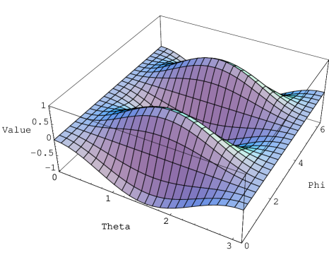
Figure 2: Angular dependence of the response function for the third polarization, adapted from Ref. [59]

For a sake of completeness, it is better to show similar figures for the cases of $+$ and $\times$ tensor GWs to compare with figure 2 [20]. The angular dependences $(1+\cos^{2}\theta)\cos 2\phi$ for the $+$ polarization and $-\cos\theta\sin 2\vartheta$ for the $\times$ polarization are respectively shown in figure 3 and figure 4.

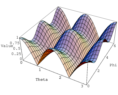
Figure 3: the angular dependence $(1+\cos^{2}\theta)\cos 2\phi$ for the $+$ polarization

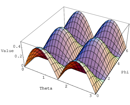
Figure 4: the angular dependence $-\cos\theta\sin 2\vartheta$ for the $\times$ polarization

5 Detectability of the magnetic component

The discussion of previous Section concerns only the low-frequency approximation of the electric component of Eqs. (58). For a better approximation in the response function one needs a frequency dependence by considering the magnetic component of Eqs. (59) too. We emphasize that in this Section 5 and in Section 6, we will consider only the magnetic component of scalar GWs. Notice that we are not claiming that the electric component can be neglected [20]. The electric component is always present. The key point is that we have discusses his potential detection in Section 3. But, as we are within the linearized theory, we can invoke the Principle of Superposition in order to discuss them separately. The same happens when one discusses separately the various different polarizations.

To compute the response functions for an arbitrary propagating direction of the GW a spatial rotation of the coordinate system has to be performed [7, 43]:

$$\begin{array}[]{ccc}u&=&-x\cos\theta\cos\phi+y\sin\phi+z\sin\theta\cos\phi\\ \\ v&=&-x\cos\theta\sin\phi-y\cos\phi+z\sin\theta\sin\phi\\ \\ w&=&x\sin\theta+z\cos\theta,\end{array}$$ (69)

or, in terms of the $x,y,z$ frame:

$$\begin{array}[]{ccc}x&=&-u\cos\theta\cos\phi-v\cos\theta\sin\phi+w\sin\theta\\ \\ y&=&u\sin\phi-v\cos\phi\\ \\ z&=&u\sin\theta\cos\phi+v\sin\theta\sin\phi+w\cos\theta.\end{array}$$ (70)

The test masses are the beam splitter and the mirror of the interferometer, and we will suppose the the beam splitter located in the origin of the coordinate system. In this way, Eqs. (59) represent the motion of the mirror like it is due to the magnetic component of the SGW.

As the mirror of Eqs. (59) is situated in the $u$ direction, using Eqs. (59), (69) and (70) the $u$ coordinate of the mirror is given by

$$u=L+\frac{1}{4}L^{2}A\dot{\Phi}(t),$$ (71)

where

$$A\equiv 2\cos\theta\cos\phi[(\frac{1+\sin^{2}\theta}{2})+\sin^{2}\theta\sin 2\phi]-2\sin^{2}\phi\sin\theta\cos\phi$$ (72)

and $L=\sqrt{l_{1}^{2}+l_{2}^{2}+l_{3}^{2}}$ is the length of the interferometer arms.

The computation for the $v$ arm is similar to the one above. Using Eqs. (59), (69) and (70), the coordinate of the mirror in the $v$ arm is:

$$v=L+\frac{1}{4}L^{2}B\dot{\Phi}(t),$$ (73)

where

$$B\equiv 2\cos\theta\sin\phi[(\frac{1+\sin^{2}\theta}{2})+\sin^{2}\theta\sin 2\phi]-2\cos^{2}\phi\sin\theta\sin\phi.$$ (74)

Equations (71) and (73) represent the distance of the two mirrors of the interferometer from the beam-splitter in presence of the scalar GW polarization (again note that only the contribution of the magnetic component of the third polarization of the GW is taken into account).

A “signal” can also be defined in the time domain (i.e. $T=L$ in our notation):

$$\frac{\delta T(t)}{T}\equiv\frac{u-v}{L}=\frac{1}{4}L(A-B)\dot{\Phi}(t).$$ (75)

The quantity (75) can be computed in the frequency domain using the Fourier transform of $\Phi$, defined by [3]

$$\tilde{\Phi}(\omega)=\int_{-\infty}^{\infty}dt\Phi(t)\exp(i\omega t),$$ (76)

obtaining

$$\frac{\tilde{\delta}T(\omega)}{T}=H_{magn}^{\Phi}(\omega)\Phi(\omega),$$

where the function

$$\begin{array}[]{c}H_{magn}^{\Phi}(\omega)=-\frac{1}{8}i\omega L(A-B)=\\ \\ -\frac{1}{4}i\omega L\{\cos\theta[(\frac{1+\sin^{2}\theta}{2})+\sin^{2}\theta\sin 2\phi](\cos\phi-\sin\phi)+\\ \\ +\sin\theta[\cos^{2}\phi\sin\phi-\sin^{2}\phi\cos\phi]\}\end{array}$$ (77)

is the total response function of the interferometer for the magnetic component of the third polarization of the scalar GW. This response function is different from the result of [43] because we corrected the error in Eqs. (20) of [43] (Eqs. (55) in this paper) and we used the correct Eqs. (56). Such an error was dragged along all the computations in [43] and this enabled incorrect geometric factors in the response function in [43].

6 A more precise response function for the magnetic component

Again, it is important to stress the importance of the magnetic component at high frequency [20]. In fact, it is well known that the frequency-range for earth based gravitational antennas is the interval $10Hz\leq f\leq 10KHz$ [1]. As we recalled in the introduction, the magnetic contribution represents the finite-wavelength correction to the usual infinite-wavelength approximation. In other words, it becomes important at high frequencies, i.e, frequencies at order KHzs [38, 39, 40, 41, 42, 43]. Thus, in this Section a more precise response function for the magnetic component at high frequency will be obtained.

Following [3, 19, 60, 61, 62], a good way to analyse variations in the proper distance (time) is by means of “bouncing photons”. A photon can be launched from the interferometer’s beam-splitter to be bounced back by the mirror. The “bouncing photons analysis” was created in [61]. Actually, it has strongly generalized to angular dependences and scalar waves in [3, 19, 60, 62]. However, this is the first time that the such a “bouncing photons analysis” is applied to the magnetic component of scalar GWs.

We start by considering a photon which propagates in the $u$ axis, but the analysis is almost the same for a photon which propagates in the $v$ axis. By using eq. (71), the unperturbed coordinates for the beam-splitter and the mirror are $u_{b}=0$ and $u_{m}=L$. Thus, the unperturbed propagation time between the two masses is

$$T=L.$$ (78)

From eq. (71), the displacements of the two masses under the influence of the GW are

$$\delta u_{b}(t)=0$$ (79)

and

$$\delta u_{m}(t)=\frac{1}{4}L^{2}A\dot{\Phi}(t+L\sin\theta\cos\phi).$$ (80)

In this way, the relative displacement in the $u$ direction, which is defined by

$$\delta L(t)=\delta u_{m}(t)-\delta u_{b}(t)$$ (81)

gives a “signal” in the $u$ direction

$$\frac{\delta T(t)}{T}|_{u}=\frac{\delta L(t)}{L}=\frac{1}{4}LA\dot{\Phi}(t+L\sin\theta\cos\phi).$$ (82)

But, for a large separation between the test masses (in the case of Virgo the distance between the beam-splitter and the mirror is three kilometres, four in the case of LIGO), the definition (81) for relative displacements becomes unphysical because the two test masses are taken at the same time and therefore cannot be in a casual connection [61, 62]. In this way, the correct definitions for the bouncing photon are

$$\delta L_{1}(t)=\delta u_{m}(t)-\delta u_{b}(t-T_{1})$$ (83)

and

$$\delta L_{2}(t)=\delta u_{m}(t-T_{2})-\delta u_{b}(t),$$ (84)

where $T_{1}$ and $T_{2}$ are the photon propagation times for the forward and return trip correspondingly. According to the new definitions, the displacement of one test mass is compared with the displacement of the other at a later time to allow for finite delay from the light propagation. The propagation times $T_{1}$ and $T_{2}$ in Eqs. (83) and (84) can be replaced with the nominal value $T$ because the test mass displacements are already first order in $\dot{\Phi}$ [62]. Thus, the total change in the distance between the beam splitter and the mirror in one round-trip of the photon is

$$\delta L_{r.t.}(t)=\delta L_{1}(t-T)+\delta L_{2}(t)=2\delta u_{m}(t-T)-\delta u_{b}(t)-\delta u_{b}(t-2T),$$ (85)

and in terms of the amplitude of the scalar GW:

$$\delta L_{r.t.}(t)=\frac{1}{2}L^{2}A\dot{\Phi}(t+L\sin\theta\cos\phi-L).$$ (86)

The change in distance (86) leads to changes in the round-trip time for photons propagating between the beam-splitter and the mirror in the $u$ direction:

$$\frac{\delta_{1}T(t)}{T}|_{u}=\frac{1}{2}LA\dot{\Phi}(t+L\sin\theta\cos\phi-L).$$ (87)

In the last calculation (variations in the photon round-trip time which come from the motion of the test masses inducted by the magnetic component of the scalar GW), it has been implicitly assumed that the propagation of the photon between the beam-splitter and the mirror of our interferometer is uniform as if it were moving in a flat space-time. But the presence of the tidal forces indicates that the space-time is curved. As a result, one more effect after the first discussed, that requires spacial separation, has to be analysed [61, 62].

From equation (80) the tidal acceleration of a test mass caused by the magnetic component of the $+$ polarization of the GW in the $u$ direction is

$$\ddot{u}(t+u\sin\theta\cos\phi)=\frac{1}{4}L^{2}A\frac{\partial}{\partial t}\ddot{\Phi}(t+u\sin\theta\cos\phi).$$ (88)

Equivalently, one can say that there is a gravitational potential [22, 61, 62]:

$$V(u,t)=-\frac{1}{4}L^{2}A\int_{0}^{u}\frac{\partial}{\partial t}\ddot{\Phi}(t+l\sin\theta\cos\phi)dl,$$ (89)

which generates the tidal forces, and that the motion of the test mass is governed by the Newtonian equation [22, 61, 62]

$$\ddot{\overrightarrow{r}}=-\bigtriangledown V.$$ (90)

For the second effect one considers the interval for photons propagating along the $u$ -axis

$$ds^{2}=g_{00}dt^{2}+du^{2}.$$ (91)

The condition for a null trajectory ($ds=0$) gives the coordinate velocity of the photons [61, 62]

$$v_{p}^{2}\equiv(\frac{du}{dt})^{2}=1+2V(t,u),$$ (92)

which to first order in $\Phi$is approximated by

$$v_{p}\approx\pm[1+V(t,u)],$$ (93)

with $+$ and $-$ for the forward and return trip respectively. By knowing the coordinate velocity of the photon, one defines the propagation time for its travelling between the beam-splitter and the mirror:

$$T_{1}(t)=\int_{u_{b}(t-T_{1})}^{u_{m}(t)}\frac{du}{v_{p}}$$ (94)

and

$$T_{2}(t)=\int_{u_{m}(t-T_{2})}^{u_{b}(t)}\frac{(-du)}{v_{p}}.$$ (95)

The calculations of these integrals would be complicated because the $u_{m}$ boundaries of them are changing with time:

$$u_{b}(t)=0$$ (96)

and

$$u_{m}(t)=L+\delta u_{m}(t).$$ (97)

But, to first order in $\Phi,$ these contributions can be approximated by $\delta L_{1}(t)$ and $\delta L_{2}(t)$ (see Eqs. (83) and (84)). Thus, the combined effect of the varying boundaries is given by $\delta_{1}T(t)$ in eq. (87). Then, only the times for photon propagation between the fixed boundaries, i.e $0$ and $L$, have to be calculated. Such propagation times are denoted with $\Delta T_{1,2}$ to distinguish from $T_{1,2}$. In the forward trip, the propagation time between the fixed limits is

$$\Delta T_{1}(t)=\int_{0}^{L}\frac{du}{v(t^{\prime},u)}\approx L-\int_{0}^{L}V(t^{\prime},u)du,$$ (98)

where $t^{\prime}$ is the delay time (i.e. $t$ is the time at which the photon arrives in the position $L$, so $L-u=t-t^{\prime}$) which corresponds to the unperturbed photon trajectory:

$t^{\prime}=t-(L-u)$.

Similarly, the propagation time in the return trip is

$$\Delta T_{2}(t)=L-\int_{L}^{0}V(t^{\prime},u)du,$$ (99)

where now the delay time is given by

$t^{\prime}=t-u$.

The sum of $\Delta T_{1}(t-T)$ and $\Delta T_{2}(t)$ gives the round-trip time for photons travelling between the fixed boundaries. Then, the deviation of this round-trip time (distance) from its unperturbed value $2T$ is

$$\begin{array}[]{c}\delta_{2}T(t)=-\int_{0}^{L}[V(t-2L+u,u)du+\\ \\ -\int_{L}^{0}V(t-u,u)]du,\end{array}$$ (100)

and, using Eq. (89), it is

$$\begin{array}[]{c}\delta_{2}T(t)=\frac{1}{4}L^{2}A\int_{0}^{L}[\int_{0}^{u}\frac{\partial}{\partial t}\ddot{\Phi}(t-2T+l(1+\sin\theta\cos\phi))dl+\\ \\ -\int_{0}^{u}\frac{\partial}{\partial t}\ddot{\Phi}(t-l(1-\sin\theta\cos\phi)dl]du.\end{array}$$ (101)

Thus, the total round-trip proper distance in presence of the magnetic component of the scalar GW is:

$$T_{t}=2T+\delta_{1}T+\delta_{2}T,$$ (102)

and

$$\delta T_{u}=T_{t}-2T=\delta_{1}T+\delta_{2}T$$ (103)

is the total variation of the proper time (distance) for the round-trip of the photon in presence of the magnetic component of the scalar GW in the $u$ direction.

By using Eqs. (87), (101) and the Fourier transform of $\Phi$ defined by Eq. (76), the quantity (103) can be computed in the frequency domain as

$$\tilde{\delta}T_{u}(\omega)=\tilde{\delta}_{1}T(\omega)+\tilde{\delta}_{2}T(\omega)$$ (104)

where

$$\tilde{\delta}_{1}T(\omega)=-i\omega\exp[i\omega L(1-\sin\theta\cos\phi)]\frac{L^{2}A}{2}\tilde{\Phi}(\omega)$$ (105)

$$\begin{array}[]{c}\tilde{\delta}_{2}T(\omega)=\frac{i\omega L^{2}A}{4}[\frac{-1+\exp[i\omega L(1-\sin\theta\cos\phi)]-iL\omega(1-\sin\theta\cos\phi)}{(1-\sin\theta\cos\phi)^{2}}+\\ \\ +\frac{\exp(2i\omega L)(1-\exp[i\omega L(-1-\sin\theta\cos\phi)]-iL\omega(1+\sin\theta\cos\phi)}{(-1-\sin\theta\cos\phi)^{2}}]\tilde{\Phi}(\omega).\end{array}$$ (106)

In the above computation the derivation and translation theorems of the Fourier transform have been used. In this way the response function of the $u$ arm of our interferometer to the magnetic component of the scalar GW results

$$\begin{array}[]{c}H_{u}^{\Phi}(\omega)\equiv\frac{\tilde{\delta}T_{u}(\omega)}{L\tilde{\Phi}(\omega)}=\\ \\ =-i\omega\exp[i\omega L(1-\sin\theta\cos\phi)]\frac{LA}{2}+\\ \\ \frac{i\omega LA}{4}[\frac{-1+\exp[i\omega L(1-\sin\theta\cos\phi)]-iL\omega(1-\sin\theta\cos\phi)}{(1-\sin\theta\cos\phi)^{2}}+\\ \\ +\frac{\exp(2i\omega L)(1-\exp[i\omega L(-1-\sin\theta\cos\phi)]-iL\omega(1+\sin\theta\cos\phi)}{(-1-\sin\theta\cos\phi)^{2}}].\end{array}$$ (107)

The computation for the $v$ arm is parallel to the one above. With the same way of thinking of previous analysis, one gets variations in the photon round-trip time which come from the motion of the beam-splitter and the mirror in the $v$ direction:

$$\frac{\delta_{1}T(t)}{T}|_{v}=\frac{1}{2}LB\Phi(t+L\sin\theta\sin\phi-L),$$ (108)

while the second contribute (propagation in a curve spacetime) will be

$$\begin{array}[]{c}\delta_{2}T(t)=\frac{1}{4}L^{2}B\int_{0}^{L}[\int_{0}^{u}\frac{\partial}{\partial t}\ddot{\Phi}(t-2T+l(1-\sin\theta\sin\phi))dl+\\ \\ -\int_{0}^{u}\frac{\partial}{\partial t}\ddot{\Phi}(t-l(1-\sin\theta\sin\phi)dl]du,\end{array}$$ (109)

and the total response function of the $v$ arm for the magnetic component of the scalar GWs is given by

$$\begin{array}[]{c}H_{v}^{\Phi}(\omega)\equiv\frac{\tilde{\delta}T_{u}(\omega)}{L\ddot{\Phi}\omega)}=\\ \\ =-i\omega\exp[i\omega L(1-\sin\theta\sin\phi)]\frac{LB}{2}+\\ \\ +\frac{i\omega LB}{4}[\frac{-1+\exp[i\omega L(1-\sin\theta\sin\phi)]-iL\omega(1-\sin\theta\sin\phi)}{(1-\sin\theta\cos\phi)^{2}}+\\ \\ +\frac{\exp(2i\omega L)(1-\exp[i\omega L(-1-\sin\theta\sin\phi)]-iL\omega(1+\sin\theta\sin\phi)}{(-1-\sin\theta\sin\phi)^{2}}].\end{array}$$ (110)

The total response function for the magnetic component is given by the difference of the two response function of the two arms:

$$H_{tot}^{\Phi}(\omega)\equiv H_{u}^{\Phi}(\omega)-H_{v}^{\Phi}(\omega),$$ (111)

and using Eqs. (107) and (110) one obtains a complicated formula

$$\begin{array}[]{c}H_{tot}^{\Phi}(\omega)=\frac{\tilde{\delta}T_{tot}(\omega)}{L\tilde{\Phi}(\omega)}=\\ \\ =-i\omega\exp[i\omega L(1-\sin\theta\cos\phi)]\frac{LA}{2}+\frac{LB}{2}i\omega\exp[i\omega L(1-\sin\theta\sin\phi)]\\ \\ -\frac{i\omega LA}{4}[\frac{-1+\exp[i\omega L(1-\sin\theta\cos\phi)]-iL\omega(1-\sin\theta\cos\phi)}{(1-\sin\theta\cos\phi)^{2}}\\ \\ +\frac{\exp(2i\omega L)(1-\exp[i\omega L(-1-\sin\theta\cos\phi)]-iL\omega(1+\sin\theta\cos\phi)}{(-1-\sin\theta\cos\phi)^{2}}]+\\ \\ +\frac{i\omega LB}{4}[\frac{-1+\exp[i\omega L(1-\sin\theta\sin\phi)]-iL\omega(1-\sin\theta\sin\phi)}{(1-\sin\theta\cos\phi)^{2}}+\\ \\ +\frac{\exp(2i\omega L)(1-\exp[i\omega L(-1-\sin\theta\sin\phi)]-iL\omega(1+\sin\theta\sin\phi)}{(-1-\sin\theta\sin\phi)^{2}}],\end{array}$$ (112)

that, at lower frequencies is in perfect agreement with the result (77):

$$\begin{array}[]{c}H_{tot}^{\Phi}(\omega\rightarrow 0)=\\ \\ =-\frac{1}{4}i\omega L\{\cos\theta[(\frac{1+\sin^{2}\theta}{2})+\sin^{2}\theta\sin 2\phi](\cos\phi-\sin\phi)+\\ \\ +\sin\theta[\cos^{2}\phi\sin\phi-\sin^{2}\phi\cos\phi]\}\end{array}$$ (113)

In figure 5 the angular dependence (112) is mapped at a frequency of $9KHz$ for the Virgo interferometer ($L=3km$, see [1]). From figure 5 it is clear why we are claiming that the magnetic contribution becomes important at high frequencies: if one neglects such a contribution considering only the low-frequency approximation of the electric contribution analysed in previous literature and in Section 4 of this paper an important portion of the total integrated signal could be, in principle, lost. In fact, the lost signal could arrive at about the $15\%$ for some particular directions of the propagating GW. To well understand this point one has to compare this magnetic contribution, which is shown in figure 5, with the electric contribution which is shown in figure 2, that is sufficient only for frequencies order hundreds Hz. For higher frequencies, i.e. frequencies order kHzs, the magnetic correction is needed.

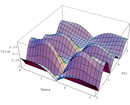
Figure 5: The angular dependence of the magnetic response function (112) at 9KHz for the Virgo interferometer ($L=3km$)

7 Comparing with General Theory of Relativity

It is important to show an expansion of the main results recalling its presence also in GRT [44]. Doing that, the importance of the STG for the effect, that is known to exist also in GRT, is further emphasized [44]. To make this, let us insert in Eqs. (57) the contribution due to the $+$ and $\times$ polarizations of the the total perturbation (44). The analogous of Eqs. (57) for the $+$ and $\times$ polarizations in GTR are Eqs. (6) of Ref. [39], which are

$$\begin{array}[]{c}x(t)=l_{1}+\frac{1}{2}[l_{1}h_{+}(t)-l_{2}h_{\times}(t)]+\frac{1}{2}l_{1}l_{3}\dot{h}_{+}(t)+\frac{1}{2}l_{2}l_{3}\dot{h}_{\times}(t)\\ \\ y(t)=l_{2}-\frac{1}{2}[l_{2}h_{+}(t)+l_{1}h_{\times}(t)]-\frac{1}{2}l_{2}l_{3}\dot{h}_{+}(t)+\frac{1}{2}l_{1}l_{3}\dot{h}_{\times}(t)\\ \\ z(t)=l_{3}-\frac{1}{4}(l_{1}^{2}-l_{2}^{2})\dot{h}_{+}(t)+2l_{1}l_{2}\dot{h}_{\times}(t).\end{array}$$ (114)

These equations, which are also Eqs. (13) of Ref. [38] written with different notations, define the motion of the mass due to the $+$ and $\times$ polarizations in the same frame of the local observer of Eqs. (57).

Neglecting the terms with $\dot{h}_{+}$ and $\dot{h}_{\times}$ in eqs. (114), the “traditional” equations for the mass motion in GTR are obtained [38, 39]:

$$\begin{array}[]{c}x(t)=l_{1}+\frac{1}{2}[l_{1}h_{+}(t)-l_{2}h_{\times}(t)]\\ \\ y(t)=l_{2}-\frac{1}{2}[l_{2}h_{+}(t)+l_{1}h_{\times}(t)]\\ \\ z(t)=l_{3}.\end{array}$$ (115)

Clearly, this is the analogous of the electric component of motion in electrodynamics [38, 39], while equations

$$\begin{array}[]{c}x(t)=l_{1}+\frac{1}{2}l_{1}l_{3}\dot{h}_{+}(t)+\frac{1}{2}l_{2}l_{3}\dot{h}_{\times}(t)\\ \\ y(t)=l_{2}-\frac{1}{2}l_{2}l_{3}\dot{h}_{+}(t)+\frac{1}{2}l_{1}l_{3}\dot{h}_{\times}(t)\\ \\ z(t)=l_{3}-\frac{1}{4}(l_{1}^{2}-l_{2}^{2})\dot{h}_{+}(t)+2l_{1}l_{2}\dot{h}_{\times}(t),\end{array}$$ (116)

are the analogue of the magnetic component of motion [38, 39]. Starting from Eqs. (116), a careful analysis has been realized in [39] where the response functions for the magnetic components in GTR have been computed [20]. In particular, the analogous of Eq. (77) for the $+$ and $\times$ polarizations are respectively [39]

$$\begin{array}[]{c}H_{magn}^{+}(\omega)=-\frac{1}{8}i\omega L(A-B)=\\ \\ =-\frac{1}{4}i\omega L\sin\theta[(\cos^{2}\theta+\sin 2\phi\frac{1+\cos^{2}\theta}{2})](\cos\phi-\sin\phi)\end{array}$$ (117)

and

$$\begin{array}[]{c}H_{magn}^{\times}(\omega)=-i\omega T(C-D)=\\ \\ =-i\omega L\sin 2\phi(\cos\phi+\sin\phi)\cos\theta.\end{array}$$ (118)

By invoking the Principle of Superposition, we can add the motion of the mass due to the third scalar polarization $\Phi$, which is defined by Eqs. (57), to the motion of the to mass due to the $+$ and $\times$ polarizations, which is defined by Eqs. (114). At the end we get

$$\begin{array}[]{c}x(t)=l_{1}+\frac{1}{2}[l_{1}h_{+}(t)-l_{2}h_{\times}(t)]+\frac{1}{2}l_{1}l_{3}\dot{h}_{+}(t)+\frac{1}{2}l_{2}l_{3}\dot{h}_{\times}(t)+\frac{1}{2}l_{1}\Phi(t)+\frac{1}{2}l_{1}l_{3}\dot{\Phi}(t)\\ \\ y(t)=l_{2}-\frac{1}{2}[l_{2}h_{+}(t)+l_{1}h_{\times}(t)]-\frac{1}{2}l_{2}l_{3}\dot{h}_{+}(t)+\frac{1}{2}l_{1}l_{3}\dot{h}_{\times}(t)+\frac{1}{2}l_{2}\Phi(t)+\frac{1}{2}l_{2}l_{3}\dot{\Phi}(t)\\ \\ z(t)=l_{3}-\frac{1}{4}(l_{1}^{2}-l_{2}^{2})\dot{h}_{+}(t)+2l_{1}l_{2}\dot{h}_{\times}(t)-\frac{1}{4}(l_{1}^{2}+l_{2}^{2})\dot{\Phi}(t).\end{array}$$ (119)

These equations define the motion of the mass due to all the three $+$, $\times$ and $\Phi$ polarizations of GWs in STG.

Thus, one can interpret the linearized scalar field $\Phi$ like a small quantity that measures the scalar sector in STG, so that when the expansion parameter vanishes one goes over to GTR [44].

8 Conclusions

In the framework of the potential detection of GWs, the important issue of the magnetic component of GWs has been considered in various paper in the literature. The analyses on this issue have shown that such a magnetic component results particularly important in the high frequency portion of the frequency range of ground based interferometers for GWs which arises from standard GTR. On the other hand, detectors for GWs will be important also because the interferometric GWs detection will be the definitive test for GTR or, alternatively, a strong endorsement for ETG. In fact, recently, the magnetic component has been extended to GWs arising from STG, which is an alternative candidate to GTR. After a review of some important issues on GWs in STG, in this paper the magnetic component has been re-analysed in from a different point of view, by correcting an error in a previous paper and by releasing a more precise response function. In this way, we have also shown that if one neglects the magnetic contribution considering only the low-frequency approximation of the electric contribution, an important portion of the signal could be, in principle, lost. In fact, the lost signal could arrive at about the $15\%$ for some particular directions of the propagating GW as it is clear by comparing the total magnetic contribution, which is shown in figure 5, with the electric contribution which is shown in figure 2.

At the end of the paper an expansion of the main results has been also shown. This point is important in order to emphasize the presence of the magnetic component in GRT too.

9 Acknowledgements

The Institute for Theoretical Physics and Mathematics Einstein-Galilei and the R. M. Santilli Foundations have to be thanked for supporting this research. I thank Herman Mosquera Cuesta, Jeremy Dunning-Davies and Mariafelicia De Laurentis for the useful discussions. Finally, I have to thank a lot the referees A and B for useful comments and advices and the referee D for his enlightening correction to the error in Eqs. (55). The excellent work of these referees permitted to strongly improve this paper.

References

- [1] The LIGO Scientific Collaboration, Class. Quant. Grav. 26, 114013 (2009)
- [2] R.A. Hulse and J.H. Taylor - Astrophys. J. Lett. 195, 151 (1975)
- [3] C. Corda - Int. Journ. Mod. Phys. D, 18, 14, 2275-2282 (2009, Honorable Mention, Gravity Research Foundation)
- [4] A. Einstein, Sitz. Kon. Preu. Akad. Wiss. 1915, 778-786
- [5] A. Einstein, Sitz. Kon. Preu. Akad. Wiss. 1916, 688-696
- [6] A. Einstein, Sitz. Kon. Preu. Akad. Wiss. 1918, 154-157
- [7] L. Iorio and C. Corda, Op. Astr. Journ. 3, 172-185 (2010), pre-print on arXiv:1001.3951
- [8] G. F. Smoot and P. J. Steinhardt, Gen. Rel. Grav. 25, 1095-1100 (1993)
- [9] L. P. Grishchuk, JETP 40, 409-415 (1975)
- [10] A. A. Starobinskii, JETPL 30, 682-685 (1979)
- [11] B. Allen, in J. A. Marck, J. P. Lasota, Eds. Relativistic Gravitation and Gravitational Radiation, pp. 373-417, Cambridge University Press, Cambridge (1997)
- [12] D. H. Lyth and A. R. Liddle, Primordial Density Perturbation, Cambridge University Press, Cambridge (2009)
- [13] D. N. Spergel et al, Astrop. J. Suppl. 148, 175-194 (2003)
- [14] F. A. E. Pirani, Phys. Rev., 105, 1089-1099 (1957)
- [15] J. Weber, Gravitational Waves. First Award at the Gravity Research Foundation Competion. Available www.gravityresearchfoundation.org
- [16] J. Weber, Phys. Rev. 117, 306-313 (1960) C. Corda - Astropart. Phys. 28, 247-250 (2007)
- [17] J. Weber, Phys. Rev. Lett. 22, 1320-1324 (1969) M. Rakhmanov - Phys. Rev. D 71 084003 (2005)
- [18] A. Giazotto, Journ. of Phys., Conf. Series 120, 032002 (2008)
- [19] C. Corda, Mod. Phys. Lett. A22, 1727-1735 (2007)
- [20] Private communication with the first referee
- [21] L. Landau L and E. Lifsits - Classical Theory of Fields (3rd ed.). London: Pergamon. ISBN 0-08-016019-0. Vol. 2 of the Course of Theoretical Physics (1971)
- [22] C. W. Misner , K. S. Thorne and J. A. Wheeler, Gravitation , W.H.Feeman and Company (1973)
- [23] H. Nicolai, G. F. R. Ellis, A. Ashtekar and others, Special Issue on quantum gravity, Gen. Rel. Grav. 41, 4, 673-1011 (2009)
- [24] A. De Felice and S. Tsujikawa, Liv. Rev. Rel. 13, 3 (2010)
- [25] T. Damour and G. Esposito-Farese, Class. Quant. Grav. 9, 2093-2176 (1992)
- [26] P. Jordan, Naturwiss. 26, 417 (1938)
- [27] M. Fierz, Phys. Acta 29, 128 (1956)
- [28] C. Brans and R. H. Dicke, Phys. Rev. 124, 925 (1961)
- [29] P. J. E. Peebles and B. Ratra, Rev. Mod. Phys. 75, 8559 (2003)
- [30] S. DeDeo, D. Psaltis, Phys. Rev. Lett. 90, 141101 (2003)
- [31] H. Sotani and K.D. Kokkotas, Phys. Rev. D 70, 084026 (2004)
- [32] H. Sotani and K.D. Kokkotas, Phys. Rev. D 71, 124038 (2005)
- [33] P. D. Lasky, H. Sotani, D. Giannios, Phys. Rev. D 78, 104019 (2008)
- [34] S. Desai, E.O. Kahya and R.P. Woodard, Phys. Rev. D, 124041 (2008)
- [35] H. Sotani, Phys. Rev. D 79, 064033 (2009)
- [36] H. Sotani, Phys. Rev. D 80, 064035 (2009)
- [37] H. Sotani, Phys. Rev. D, 81, 084006 (2010)
- [38] D. Baskaran and L. P. Grishchuk, Class. Quant. Grav. 21, 4041-4061 (2004)
- [39] C. Corda, Int. J. Mod. Phys. D 16, 9, 1497-1517 (2007)
- [40] C. Corda, Int. J. Mod. Phys. A 22, 2361 (2007)
- [41] L. Iorio and C. Corda, AIP Conf. Proc. 1168, 1072-1076 (2009)
- [42] C. Corda, Proceedings of the XLIInd Rencontres de Moriond, Gravitational Waves and Experimental Gravity, p. 95, Ed. J. Dumarchez and J. T. Tran, Than Van, THE GIOI Publishers (2007)
- [43] C. Corda, S. A. Ali, C. Cafaro, Int. Journ. Mod. Phys. D 19, 13, 2095 (2010)
- [44] Private communication with the second referee
- [45] H. Stephani et al., Exact Solutions of Einstein’s Field Equations, Cambridge University Press, 2nd edition (2003)
- [46] L. F. Costa and C. A. R. Herdeiro, Phys. Rev. D 8, 024021 (2008)
- [47] C. Corda, Astropart. Phys. 34, 412 (2011)
- [48] S. W. Hawking and G. F. R. Ellis, The large scale structure of spacetime, Cambridge University Press (1973)
- [49] M. F. Bennett, C. A. Van Eysden, and A. Melatos, Mon. Not. Roy. Astron. Soc., Article first published online: 14 SEP 2010, DOI: 10.1111/j.1365-2966.2010.17416.x
- [50] X. J. Zhu, E. Howell, D. Blair, Mon. Not. Roy. Astron. Soc. 409, L132-L136 (2010)
- [51] Abbot et al., Nature 460, 990-994 (2009)
- [52] M. E. Tobar, T. Suzuki and K. Kuroda, Phys. Rev. D 59 102002 (1999)
- [53] P. D. Scharre and C. M. Will, Phys. Rev. D 65, 042002 (2002)
- [54] J. Novak, and J.M. Ibanez, Astrophys. J. 533, 392-405 (2000)
- [55] C. Will - Liv. Rev. Rel. 4, 4 (2001) updated at Publication URI: http://www.livingreviews.org/lrr-2006-3 (2006)
- [56] R. M. Wald - General Relativity - The Universiy Chicago Press, Chicago (1984)
- [57] Y.M. Cho - Phys. Rev. Lett. 68, 3133 (1992)
- [58] N. Bonasia and M. Gasperini, Phys. Rev. D 71, 104020 (2005)
- [59] C. Corda, Astropart. Phys. 28, 247-250 (2007)
- [60] C. Corda, Astropart. Phys. 27, 539-549 (2007)
- [61] M. Rakhmanov, Phys. Rev. D 71 084003 (2005)
- [62] C. Corda, Journ. Cosm. Astr. Phys. 0704:009 (2007)
- [63] Private communication with the fourth referee
- [64] D. Babusci, L. Baiotti, F. Fucito, A. Nagar, Phys. Rev. D 64 062001 (2001)
- [65] B. Allen, Proceedings of the Les Houches School on Astrophysical Sources of Gravitational Waves, pp. 373-417 eds. Jean-Alain Marck and Jean-Pierre Lasota, Relativistic Gravitation and Gravitational Radiation. Cambridge University Press (1997)