The conic-gearing image of a complex number
and a spinor-born surface geometry

Alexander P. Yefremov
Institute of Gravitation and Cosmology of Peoples’ Friendship University of Russia
6 Miklukho-Maklaya St., Moscow 117198, Russia

Quaternion (Q-) mathematics formally contains many fragments of physical laws; in particular, the Hamiltonian for the Pauli equation automatically emerges in a space with Q-metric. The eigenfunction method shows that any Q-unit has an interior structure consisting of spinor functions; this helps us to represent any complex number in an orthogonal form associated with a novel geometric image (the conic-gearing picture). Fundamental Q-unit-spinor relations are found, revealing the geometric meaning of spinors as Lamé coefficients (dyads) locally coupling the base and tangent surfaces.

1 Introduction

Among hardly conceived physical objects, like the electric charge or the elementary particle spin, the most mysterious champion is probably the quantum-mechanical wave function. Providing extremely precise predictions of real phenomena, the theory of quantum mechanics remains in many aspects a “given-by-heavens” perfect computing technology with a “noumenon” essence. Difficulties to reveal the essence have eventually overwhelmed attempts to endow the wave function with a geometrically conceivable image, and the majority of physicists of the 20th century conceded at its interpretation as a probability amplitude. A similar lack of understanding exists with spinor functions, relativistic extensions of the wave function, in the theory of Dirac or Weyl fermion fields. Indeed, human mind has usually no trouble in creating visual models of scalar, vector and maybe some tensor objects, but “a square root from a vector” (which a spinor mathematically is) makes the imagination fail.

A search for a better perception of physical laws follows nowadays some new ways; one of them is a thorough investigation of hypercomplex (H-) numbers. Among the latest examples one can cite the “perplex” (split-complex, double) numbers used to formulate 2-dimensional Lorentz-Minkowski relations [1] and the bi-quaternion (BQ-) numbers whose algebra is noticed to contain the basic formulas of relativity theory as its fundamental part [2, 3]. A closer view reveals at least two advantages of the H-number approach, especially that of quaternions. First, these numbers, the from times of Hamilton, their inventor [4], are recognized to be “very geometric,” giving clear vector images for the physical objects they are attributed to. Second, being represented by square matrices the numbers are found to be closely linked to the spinors.

But there is one more advantage. Investigation of the whole set of H-numbers helps one to think of the formerly well-known simpler numbers as of a particular case of the set, and this may lead to surprising results. Representatives the of algebra of complex (C-) numbers are such doubtlessly known simpler numbers with their famous geometrical images on Wessel’s complex plane or on Riemann’s sphere. Nonetheless, it is shown below that a C-number regarded as a special quaternion, apart from its “old” properties, possesses some new features including an original geometric image. Written in the matrix form, the C-number is proved to inevitably have an interior structure whose elements are spinor functions. The functions further on are discovered to behave as dyad coefficients linking differentials of coordinates to a couple of specific 2-dimensional (2D) surfaces.

In Section II, a short review of H-number sets is given with necessary remarks on the stability of the numbers’ multiplication table. In Section III, a C-number is treated as a dimensionally reduced quaternion in a matrix form, and its structural elements are investigated in detail. Section IV is devoted to a geometric interpretation of the C-number, its basic elements, and their graphic realization. Section V deals with a comparison of properties of the new geometry with those of spinors. The compact Section VI concludes the study.

2 Units of quaternion numbers and the Pauli spin term

Frobenius’ famous theorem states that the algebra of Hamilton’s quaternions is the largest one in the number of basic units (four units with real coefficients) that admits a non-communicative but still associative multiplication (over addition). The next, by the number of dimensions, algebra of octonions (Kaylay’s algebra, eight units) has non-associative multiplication. The most extended associative algebra is that of BQ-numbers built on Q-units, but with C-number coefficients at them. This algebra is not a “good one” since the norm of its numbers is not in general definable, and moreover, it contains zero-devisors. The BQ-algebra encompasses all other associative algebras: those of Q-numbers, C- and real numbers (good algebras), and two “exotic” algebras of split-complex and dual numbers, both with zero-devisors [5]. Let us recall here the main properties of Q-units, the base of all these sets.

The BQ- and Q- algebras are based on one real (scalar) and three imaginary (vector) units {$1;{\bf i,j,k}$} with the following 16 equalities of the multiplication table postulated by Hamilton:

$${}1^{2}=-{\bf i}^{2}=-{\bf j}^{2}=-{\bf k}^{2}=1,$$

$${}{\bf i}1=1{\bf i}={\bf i},\ \ \ {\bf j}1=1{\bf j}={\bf j},\ \ \ {\bf k}1=1{\bf k}={\bf k},$$

$${}{\bf i}{\bf j}=-{\bf j}{\bf i}={\bf k},\ \ \ {\bf j}{\bf k}=-{\bf k}{\bf j}={\bf i},\ \ \ {\bf k}{\bf i}=-{\bf i}{\bf k}={\bf j}.$$ (1)

If the units are written in the shorter (tensor) form

$${}{\bf i}={\bf q}_{1},\ \ \ {\bf j}={\bf q}_{2},\ \ \ {\bf k}={\bf q}_{3},$$

$${}\{1,{\bf i,j,k}\}\mapsto\{1,{\bf q}_{k}\},$$ (2)

with small Latin indices $k,l,m,n...=1,2,3$, then the bulky set (1) is reduced to

$$1{\bf q}_{k}={\bf q}_{k}1={\bf q}_{k},\ \ \ {\bf q}_{k}{\bf q}_{n}=-\delta_{kn}+\varepsilon_{knm}{\bf q}_{m},$$ (3)

where $\delta_{kn}$ is the 3D Kronecker symbol, $\varepsilon_{knm}$ is totally skew-symmetric 3D Levi-Civita symbol, and summing in repeated indices is implied. The multiplication table (3) is convenient for an analysis of its stability (form-invariance) under transformations of Q-units; it turns out that there are two types of admissible transformations of the vector units, the scalar unit remaining intact [2]. The first type is the rotational (vector-type) transformation

$${\bf q}_{k^{\prime}}=O_{k^{\prime}n}{\bf q}_{n}$$ (4)

where $O_{k^{\prime}n}$ is a $3\times 3$-matrix with components being in general C-numbers. After substitution of Eq. (4) into Eq. (3), the form of the multiplication rule (3) is preserved if the matrix $O_{k^{\prime}n}$ satisfies the orthogonality condition

$$O_{k^{\prime}n}O_{m^{\prime}n}=\delta_{km};$$ (5)

this means that all transformations of the type (4) form the special orthogonal group of 3D rotations over the field of C-numbers: $O_{k^{\prime}n}\in SO(3,C)$. The second type of transformations (reflections) that can give the same Q-triad (4) is performed by the operator $U$ and its inverse $U^{-1}$:

$${\bf q}_{k^{\prime}}=U{\bf q}_{k}U^{-1};$$ (6)

one immediately verifies that the transformation (6) does not change the form of the rule (3). The operators $U$ are known to form the group of special linear 2D transformations over the field of C-numbers, i.e., $U\in SL(2,C)$ (the spinor group), and this spinor group is 2:1 isomorphic to $SO(3,C)$ and similarly to the Lorentz group. Thus the Q- (and BQ-) basis (2), a pure algebraic object, turns out to be tightly linked to geometry and physics: vectors, rotations, spinors, and transformations of special relativity.

The Q-units satisfying the rules (3) can be described in terms of real and complex numbers, but these numbers should be components of square matrices. A simple $2\times 2$ matrix representation had been (up to a constant factor) proposed by Pauli, this representation is considered to be canonical:

$${}1=\left(\begin{array}[]{cc}{1}&{0}\\ {0}&{1}\end{array}\right),\qquad{\bf q}_{1}=-i\left(\begin{array}[]{cc}{0}&{1}\\ {1}&{0}\end{array}\right),$$ (11)

$${}{\bf q}_{2}=-i\left(\begin{array}[]{cc}{0}&{-i}\\ {i}&{0}\end{array}\right),\quad{\bf q}_{3}=-i\left(\begin{array}[]{cc}{1}&{0}\\ {0}&{-1}\end{array}\right);$$ (16)

other samples can be obtained with the help of the transformations (4) or (6).

Quaternions are in many ways linked to descriptions of physical laws, not only as a good tool but also as a “math-medium” where the physical relations known from experiment or formulated heuristically are surprisingly found. Apart from the above-mentioned connection with special relativity, a famous “quaternion coincidence” was revealed by Fueter [6] who discovered that the Cauchy-Riemann-like differentiability conditions for vector functions of a quaternion variable, pure mathematical requirements, are an exact formal equivalent of the full set of the vacuum Maxwell equations. Another striking example is the Pauli quantum-mechanical Hamiltonian computed in the Q-metric. Let an electron with mass $m$ and electric charge $e$ in an exterior magnetic field with the vector potential $A_{k}$, thus having the generalized momentum

$$P_{k}=p_{k}-\frac{e}{c}A_{k},\qquad p_{k}=-i\hbar\nabla_{k},$$ (17)

move in space with the quaternion metric being, up to the sign, the tensor part of the Q-multiplication rule (3):

$${\bf g}_{kn}\equiv-{\bf q}_{k}{\bf q}_{n}=\delta_{kn}-\varepsilon_{knm}{\bf q}_{m}.$$ (18)

Then it is an easy exercise [7] to find that the Hamiltonian operator computed for this particle automatically comprises the initially heuristic Pauli spin term with a coefficient precisely coinciding with the Bohr magneton,

$${}H\equiv{\bf g}_{kn}P_{k}P_{n}\ \ \mapsto\hskip 72.26999pt$$

$${}\hskip 28.45274ptH=\frac{1}{2m}\left({\bf p}-\frac{e}{c}{\bf A}\right)^{2}-\frac{e\hbar}{2mc}{\bf B}\mbox{\boldmath$\sigma$};$$ (19)

here the traditional 3D vector notations are used, $p_{k}\mapsto{\bf p}$, $A_{k}\mapsto{\bf A}$, ${\bf B}={\rm curl}\,{\bf A}$, where $-i{\bf q}_{k}\mapsto\mbox{\boldmath$\sigma$}$ are the Pauli matrices. Introduction of the Pauli operator (2) compels to replace the former “scalar” wave function of the electron with a 2D function-column, in fact a spinor.

3 Complex numbers in a matrix form and their structure

A C-number

$$z=x+iy$$ (20)

can be regarded as a quaternion having nonzero real coefficients ($x,y\in{\mathbb{R}}$) at the real unit 1 and at only one of the vector units $i\to{\bf q}$,

$$z=x\cdot 1+y\cdot{\bf q}.$$ (21)

One directly proves that each $2\times 2$ matrix of the generic form

$${\bf q}=\frac{i}{\sqrt{T}}\left(\begin{array}[]{cc}{a}&{b}\\ {c}&{-a}\end{array}\right)$$ (22)

is an imaginary unit such that

$${\bf q}^{2}=-\left(\begin{array}[]{cc}{1}&{0}\\ {0}&{1}\end{array}\right)=-1$$ (23)

if

$$T\equiv a^{2}+bc,$$ (24)

the components of the matrix (22) being in general C-numbers (or functions) $a,b,c\in{\mathbb{C}}$, with the scalar “interior imaginary unit” $i$ involved only in the structure of ${\bf q}$. The unit (22) is readily reduced to any of the vector units from the set (11), and vice versa, it can be obtained from the vector units of the set (11) using the transformations (4) or (6).

Thus Eqs. (21), (22) give a generic $2\times 2$ matrix form of C-numbers obeying all laws of the C-algebra (the existence of summation, communicative an associative multiplication, division, conjugation, modulus, etc.). But unlike the traditional scalar description, a complex number in the form (21) can be shown to have an elegant interior structure revealed in study of eigenfunctions of the matrix (22) treated as an operator.

The operator (22) may have left (2D rows $\varphi$) and right (2D columns $\psi$) eigenfunctions (EF) satisfying the equations

$$\varphi{\bf q}=k\varphi,\qquad{\bf q}\psi=l\psi,$$ (25)

with the eigenvalues $k,l$. After simple algebra, one arrives at two sets of general solutions of Eqs. (25) $\varphi^{+},\ \psi^{+}$ and $\varphi^{-},\psi^{-}$ attributed to positive

$$k^{+}=l^{+}=+i,$$ (26)

and negative

$$k^{-}=l^{-}=-i,$$ (27)

eigenvalues, respectively:
for $a\neq T$:

$$\varphi^{\pm}=\frac{1}{\sqrt{2T}}\left(\sqrt{T\mp a},\ \mp\frac{b}{\sqrt{T\mp a}}\right),$$

$$\psi^{\pm}=\frac{1}{\sqrt{2T}}\left(\begin{array}[]{c}{\sqrt{T\mp a}}\\ {\mp\frac{c}{\displaystyle\sqrt{T\mp a}}}\end{array}\right);$$

for $a=T,\ b=0$:

$$\varphi^{+}=(-c/2,\,1),\ \ \ \varphi^{-}=(1,\,0),$$

$$\psi^{+}=\left(\begin{array}[]{c}{0}\\ {1}\end{array}\right),\psi^{-}=\left(\begin{array}[]{c}{1}\\ {c/2}\end{array}\right);$$

for $a=T,c=0$:

$$\varphi^{+}=(0,\,1),\ \ \ \varphi^{-}=(1,\,b/2),$$

$$\psi^{+}=\left(\begin{array}[]{c}{-b/2}\\ {1}\end{array}\right),\psi^{-}=\left(\begin{array}[]{c}{1}\\ {0}\end{array}\right).$$

All EFs (19) possess the following properties. EFs of the same parity ($+$ or $-$) are normalized,

$$\varphi^{\pm}\psi^{\pm}=1,$$ (20)

EFs of opposite parities are automatically orthogonal:

$$\varphi^{\mp}\psi^{\pm}=0.$$ (21)

There is one more important feature: tensor products of EFs of the same parity give the two matrices

$$\psi^{+}\varphi^{+}=C^{+},\ \ \ \psi^{-}\varphi^{-}=C^{-},$$ (22)

mutually orthogonal,

$$C^{+}C^{-}=0,$$ (23)

and each having a zero determinant:

$$\det C^{\pm}=0;$$ (24)

one readily finds that any positive integer power $N$ of $C^{\pm}$ returns the initial matrix:

$$C^{\pm N}=C^{\pm},$$ (25)

hence $C^{\pm}$ are idempotent matrices. The latter property makes it easy to find form Eqs. (25) that the units 1 and ${\bf q}$ are expressed in terms of the matrices $C^{\pm}$ as

$${}1=C^{+}+C^{-}=\psi^{+}\varphi^{+}+\psi^{-}\varphi^{-},$$ (26)

$${}{\bf q}=i(C^{+}-C^{-})=i(\psi^{+}\varphi^{+}-\psi^{-}\varphi^{-}).$$ (27)

Eqs. (26) and (27) are fundamental mathematical equalities. They state that both units of the algebra of complex numbers, the real and imaginary ones, have an interior structure comprising more elementary mathematical objects. And since the imaginary unit ${\bf q}$ is one of the vector Q-units, these elementary objects, EFs, should be $SL(2,C)$, in particular $SU(\ref{yef__2_})$, spinors because the transformation (6) providing stability of the Q-multiplication table (3) is equivalent to transformations of the EFs only:

$$\psi^{\prime\pm}=U\psi^{\pm},\ \ \ \varphi^{\prime\pm}=\varphi^{\pm}U^{-1}.$$ (28)

The spinor nature of the EFs will be a crucial point in our further discussion of a novel physics-geometry link, but let us now turn to the non-traditional image of C-numbers.

4 The orthogonal form of C-numbers and the conic-gearing picture

Express the units in the C-number

$$z=x\cdot 1+y\cdot{\bf q}$$ (29)

in terms of the EFs using Eqs. (26) and (27):

$${}z=x(\psi^{+}\varphi^{+}+\psi^{-}\varphi^{-})+iy(\psi^{+}\varphi^{+}-\psi^{-}\varphi^{-})$$

$${}\hskip 28.45274pt=(x+iy)\psi^{+}\varphi^{+}+(x-iy)\psi^{-}\varphi^{-},$$ (30)

or in terms of the idempotent matrices,

$$z=(x+iy)C^{+}+(x-iy)C^{-}.$$ (31)

Eq. (31) represents the matrix C-number $z$ in an orthogonal form since a scalar C-number and its conjugate are coefficients of mutually orthogonal idempotents:

$$C^{+}C^{-}=0.$$ (32)

The number (31) is preferably rewritten in a polar format with

$${}r\equiv(x^{2}+y^{2})^{1/2},\ \ \ \alpha\equiv\arctan(y/x),$$ (33)

$${}z=r\left(e^{i\alpha}C^{+}+e^{-i\alpha}C^{-}\right).$$ (34)

Any positive integer power of $z$ evidently preserves the orthogonal form.

The bifurcation (34) deserves a graphic image that will be step-by-step constructed as follows. The idempotents $C^{+},\ C^{-}$ in a certain manner determine two orthogonal directions with attached components, each component, a scalar C-number, having its image on a complex plane. But Eq. (34) requires that there be two complex planes (two components) associated with the two orthogonal directions, hence the planes should be also conceived as being perpendicular to each other. Now temporarily fix the length $r$ of the components leaving the angle $\alpha$ variable; then the orthogonal component’s planes are reduced to circles of radius $r$, and a change in the radius angle on one circle entails an angle change of the same value but of opposite sign on the orthogonal circle. Thus the components of the number (34) behave as two mutually perpendicular discs touching at a point at their edges and able to rotate each other without slipping like a conic gear couple in a mechanical transmission (see the figure). It is obvious that a change of the discs’ radius makes the picture enlarge or shrink without changing its shape, making a conformal transformation of the graph. This is the first “direct” geometric image of the matrix C-number, but not the only one.

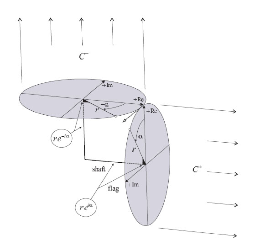
Figure 1: Conic-gearing image of a complex number

Supply the discs with “shafts”, infinitesimally thin rods connecting the discs’ centers with the central point of the graph where the rods intersect. Each rod obviously has a length equal to the disc radius $r$, and if at each rod a flag (“weathercock”) is attached marking the value of the angle $\alpha$ or -$\alpha$, then the “rod & flag” graphs contain all information about the scalar C-number and its conjugate. A couple of orthogonal rods of certain (but equal) lengths twisted about themselves and having flags indicating the angles of the twist (angles of equal value but of opposite sign) is another, suggested here, geometric image of a C-number in the orthogonal matrix form. Both geometric images are shown in the conic gearing picture (see the figure), which in this case must be 3-dimensional. A question remains about depicting the objects $C^{+}$, $C^{-}$ being matrices, not vectors, nonetheless determining directions. In fact (it will be shown in the next section), the matrices are 2D geometric projectors onto a certain direction for any vector or tensor; this hints to portraying the two projectors as two orthogonal “fluxes” of arrows in 3D space.

5 Geometry of spinors

Now it is useful to introduce two types of 2D indices. The first set of indices $A,B...=1,2$ is aimed at describing the components of $2\times 2$ matrices:

$$1\to\delta_{A}^{B},\ \ \ {\bf q}\to q_{A\cdot}^{\;B},\ \ \ C\to C_{A\cdot}^{\;B};$$ (35)

the index position is important: the lower indices count columns, the upper ones enumerate rows. The left and right spinors acquire indices with different positions, which permits denoting them by the same (new) symbol

$$\varphi\to h_{A},\ \ \ \psi\to h^{A}.$$ (36)

Indices of the second type (in parentheses), also two-dimensional $(K),(L)...=1,2$, replace the indicators of parity,

$${}\varphi^{-}\to h_{(1)A},\ \ \psi^{-}\to h_{(1)}^{B},\ \ \varphi^{+}\to h_{(2)A},\ \ \psi^{+}\to h_{(2)}^{B},$$

$${}{\rm or}\ \ \ \varphi^{\pm}\to h_{(K)A},\ \ \ \psi^{\pm}\to h_{(K)}^{B},$$ (37)

and

$$C^{\pm}\to C_{(K)A}{}^{\!B};$$ (38)

these indices will always be written at the lower position. With these notations, the normalization and orthogonality equations (20), (21) are unified in the single equality (the Kronecker delta’s indices are always used without parentheses)

$$h_{(K)A}h_{(L)}^{A}=\delta_{KL},$$ (39)

while Eq. (26) acquires the form

$$h_{(K)A}h_{(K)}^{B}=\delta_{A}^{B}.$$ (40)

Eqs. (39) and (40) help us to make an important observation: they are identical to the conditions, well-known from differential geometry, for the generic Lamé coefficients $h_{(K)A}$, $h_{(K)}^{B}$ that locally link two coordinate systems,

$$y^{A}\leftrightarrow X_{(K)},$$ (41)

belonging to two different spaces, in our case 2D surfaces,

$$dX_{(K)}=h_{(K)A}dy^{A},\ \ \ dy^{B}=h_{(K)}^{B}dX_{(K)}.$$ (42)

The surfaces are tangent in their common point, and their common squared interval is

$${}dl^{2}\equiv dy_{B}dy^{B}=h_{(K)B}h_{(L)}^{B}dX_{(K)}dX_{(L)}$$

$${}\qquad=\delta_{KL}dX_{(K)}dX_{(L)}=dX_{(1)}^{2}+dX_{(2)}^{2}.$$ (43)

Eqs. (42) and (5) state that one 2D space, having the coordinates $X_{(K)}$, possesses the Cartesian metric $\delta_{KL}$, so locally it is a plane, while the surface with the coordinates $y^{A}$ has the metric

$$g_{AB}\equiv h_{(K)A}h_{(K)B},$$ (44)

which is in fact Eq. (40) with both lowered indices. In general, the metric (44) has variable components, and the surface it describes may be curved. According to the traditions of differential geometry, the 2D manifold with the metric (44) should be called a base space, and that with the Cartesian metric a tangent plane, while the set of Lamé coefficients $h_{(K)}^{A}$ linking the 2D spaces should be named a dyad (analogously to triads in the 3D case, tetrads in the 4D case etc.).

Using the new notations, we write the idempotent matrices (22) with all lower indices:

$$C_{(1)AB}=h_{(1)A}h_{(1)B},\ \ \ C_{(2)AB}=h_{(2)A}h_{(2)B},$$ (45)

and find their components on the tangent plane; for this purpose, contract Eqs. (45) with the dyad $h_{(K)}^{A}$ using Eq. (39):

$${}C_{(1)(K)(L)}=h_{(1)A}h_{(1)B}h_{(K)}^{A}h_{(L)}^{B}=\delta_{1K}\delta_{1L},$$

$${}C_{(2)(K)(L)}=\delta_{2K}\delta_{2L}.$$ (46)

Eqs. (5) directly show that the idempotent matrices are projectors onto one of the two orthogonal direction, there sum just yielding the component development of the Cartesian metric (Kronecker delta), the tangent equivalent of Eq. (26)

$$\delta_{KL}=\delta_{1K}\delta_{1L}+\delta_{2K}\delta_{2L};$$ (47)

hence the Kronecker delta components $\delta_{1K},\delta_{2K}$ are the simplest (plane) spinors forming the tangent plane. The imaginary unit (27) written in terms of the plane spinors has the form of the imaginary Lorentz-type metric

$$q_{KL}=-i(\delta_{1K}\delta_{1L}-\delta_{2K}\delta_{2L}),$$ (48)

its components coinciding with those of the canonical Q-unit ${\bf q}_{3}$ form, Eq. (11). The plane spinors $\delta_{1K},\delta_{2K}$ are obviously eigenfunctions of the vector operator (27), but they can be used as well to build the components of any other Q-unit from Eq. (11), e.g., ${\bf q}_{2}$:

$${\bf q}_{2}\mapsto q_{LN}=\delta_{1N}\delta_{2L}-\delta_{2N}\delta_{1L}.$$ (49)

A product of Eqs. (49) and (48) gives an expression of ${\bf q}_{1}$ from Eq. (11) in terms of the plane spinors:

$${}{\bf q}_{1}={\bf q}_{2}{\bf q}_{3}\ \mapsto\ q_{KN}=q_{KL}q_{LN}$$

$${}=(\delta_{1N}\delta_{2L}-\delta_{2N}\delta_{1L})(-i)(\delta_{1K}\delta_{1L}-\delta_{2K}\delta_{2L})$$

$${}=i(\delta_{1K}\delta_{2N}+\delta_{2K}\delta_{1N}).$$ (50)

Eqs. (48)–(5) show that the plane spinors belonging to some tangent plane (in this case as Lamé coefficients linking the Cartesian systems of two planes coordinates) are at the same time elements for construction of all canonical vector Q-units (11). This establishes a direct — and quite technological — mathematical relationship between an abstract plane (a screen) and each direction of the 3D space (the physical space).

6 Concluding remarks

There are three main results of the study to be emphasized. First, the quaternion space, a natural geometric consequence of Q-algebra, gives rise to the Pauli term in the quantum-mechanical Hamiltonian of the electron. Second, the spinors, an extension of the wave function, are revealed to be structural elements of Q-units, which is a pure mathematical fact suggesting a novel geometric image of C-numbers, a dimensional reduction of quaternions. And the third significant issue of the study is establishing of a geometric meaning of the set of spinor functions, basic elements of 3D vector Q-units, as Lamé coefficients (dyads) interconnecting two mutually tangent surfaces. Investigations of variable (non-planar) spinors are expected to reveal the mutual dependence of the curved spinor-born base surface and the respective dynamic points of the 3D (physical) space endowed with a vector Q-triad. An intriguing subject is an analysis of limits on the curvature and/or regularity of the local surface that can result in discontinuity and spectrum of the dyad function thus possibly leading to a better understanding of quantum phenomena. Further explorations of fundamental structures of H-numbers will hopefully allow extending the knowledge of this surprisingly rich “math-medium” and its links with physics.

References

- [1] P. Fjelstad, Extending special relativity via the perplex numbers, Am. J. Phys. 54 (5), 416–422 (1986).
-
[2]
A. P. Yefremov, Quaternions: Algebra, geometry, and physical
theories, Hypercomplex Numbers in Geometry and Physics,
1, 104–119 (2004). Available online in
http://hypercomplex.xpsweb.com/articles
/147/en/pdf/01-10-e.pdf. - [3] A. P. Yefremov, Quaternion model of relativity: solutions for non-inertial motions and new effects, Adv. Sci. Lett. 1, 179–186 (2008).
-
[4]
W. R. Hamilton, Lectures on Quaternions (Dublin, Hodges &
Smith, 1853). Available online in
http://www.archive.org/details
/lecturesonquater00hami. - [5] A. P. Yefremov, Structure of hypercomplex units and exotic numbers as sections of bi-quaternions, Adv. Sci. Lett. 3, 537–542 (2010).
- [6] R. Fueter, Analytische Funktionen einer Quaternionenvariablen, Comm. Math. Helv. 4, 9-20 (1932).
- [7] A. P. Yefremov, Quaternionic multiplication rule and a local Q-metric, Lett. Nuovo Cim. 37 (8), 315–316 (1983).