Strongly correlated electron systems; heavy fermions Electronic structure Quantum phase transitions

High magnetic fields thermodynamics of heavy fermion metal $\rm\bf YbRh_{2}Si_{2}$.

Abstract

We perform comprehensive theoretical analysis of high magnetic field behavior of the heavy-fermion (HF) compound $\rm YbRh_{2}Si_{2}$. At low magnetic fields $B$, $\rm YbRh_{2}Si_{2}$ has a quantum critical point related to the suppression of antiferromagnetic ordering at a critical magnetic field $B\perp c$ of $B=B_{c0}\simeq 0.06$ T. Our calculations of the thermodynamic properties of $\rm YbRh_{2}Si_{2}$ in wide magnetic field range from $B_{c0}\simeq 0.06$ T to $B\simeq 18$ T allow us to straddle a possible metamagnetic transition region and probe the properties of both low-field HF liquid and high-field fully polarized one. Namely, high magnetic fields $B\sim B^{*}\sim 10$ T fully polarize corresponding quasiparticle band generating Landau Fermi liquid (LFL) state and suppressing HF (actually NFL) one, while at elevating temperatures both HF state and corresponding NFL properties are restored. Our calculations are in good agreement with experimental facts and show that the fermion condensation quantum phase transition is indeed responsible for the observed NFL behavior and quasiparticles survive both high temperatures and high magnetic fields.

An explanation of the rich and striking behavior of heavy fermion (HF) metals is, as years before, among the main problems of modern condensed matter physics. One of the most interesting and puzzling issues in the research of HF compounds is their non-Fermi liquid (NFL) behavior in a wide range of temperatures $T$ and magnetic fields $B$. For example, recent measurements of the specific heat $C$ of $\rm YbRh_{2}Si_{2}$ under the application of magnetic field $B$ show that the above temperature range extends at least up to twenty Kelvins as reported in the inset to fig. 1. As it is well-known from Landau Fermi liquid (LFL) theory, the ratio $C/T$ is proportional to quasiparticle effective mass $M^{*}$. The inset to fig. 1 reports the dependence of $C(T)/T$, which has a maximum $M^{*}_{\rm max}(B)$ at some temperature $T_{\rm max}(B)$. It is seen from the inset, that $M^{*}_{\rm max}(B)$ decreases as magnetic field $B$ grows, while $T_{\rm max}(B)$ shifts to higher $T$ reaching $15$ K at $B=18$ T [1].

A deeper insight into the behavior of $C/T$ in the inset to fig. 1 can be achieved using some ”internal” scales. Namely, near QCP it is convenient to divide the effective mass $M^{*}$ and temperature $T$ by their maximal values, $M^{*}_{\rm max}$ and $T_{\rm max}$ respectively. This generates the normalized effective mass $M^{*}_{N}=M^{*}/M^{*}_{\rm max}$ and temperature $T_{N}=T/T_{\rm max}$ [2]. In the main panel of fig. 1 the obtained dependence $M^{*}_{N}(T_{N})$ is shown by symbols, corresponding to different magnetic fields. This immediately reveals the scaling in the normalized experimental curves - the curves at different magnetic fields $B$ merge into a single one in terms of the normalized variable $T_{N}=T/T_{\rm max}$. It is seen from fig. 1, that the normalized effective mass $M^{*}_{N}(T_{N})$ is not a constant as it would be for LFL case. Rather, it shows the scaling behavior in normalized temperature $T_{N}$. It is also seen from fig. 1 (both the main panel and inset) that the NFL behavior and the associated scaling extend at least to temperatures up to twenty Kelvins.

Thus, we conclude that a challenging problem for theories considering the high magnetic field ( $B\sim B^{*}$) NFL behavior of the HF metals is to explain both the scaling and the shape of $M^{*}_{N}(T_{N})$. Another part of the problem is the remarkably large temperature and magnetic field ranges where the NFL behavior and scaling are observed.

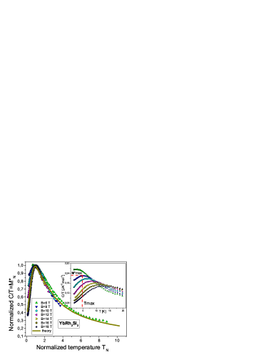
Figure 1: The normalized effective mass $M^{*}_{N}=M^{*}/M^{*}_{\rm max}$ versus normalized temperature $T_{N}=T/T_{\rm max}$. $M^{*}_{N}$ is extracted from the measurements (shown in the inset) of the specific heat $C/T$ on $\rm YbRh_{2}Si_{2}$ in magnetic fields $B$ [1] listed in the legend. Our calculations (made at $B\simeq B^{*}$ when the quasiparticle band is fully polarized) are depicted by the solid curve tracing the scaling behavior of $M^{*}_{N}$. The inset reports the temperature dependence of the electronic specific heat $C/T$ of $\rm YbRh_{2}Si_{2}$ at different magnetic fields [1] shown in the main panel legend. The illustrative values of $M^{*}_{\rm max}$ and $T_{\rm max}$ at $B=8$ T are also shown.

In this letter, based on the theory of fermion condensation quantum phase transition (FCQPT) [2] we analyze the thermodynamic properties of $\rm YbRh_{2}Si_{2}$ at both low and high magnetic fields. Our calculations of the specific heat and magnetization allow us to conclude that under the application of magnetic field the heavy-electron system of $\rm YbRh_{2}Si_{2}$ evolves continuously without a metamagnetic transition. At low temperatures and high magnetic fields $B\simeq B^{*}$ the system is completely polarized and demonstrates the LFL behavior, while at elevated temperatures the HF behavior and related NFL one are restored. The obtained results are in good agreement with experimental facts in the entire magnetic field ($0.1$ T - $18$ T) and temperature (40 mK - 20 K) domains.

In our FCQPT approach [2], to study the (generally speaking NFL) behavior of the effective mass $M^{*}(T,B)$, we simply use Landau equation for the quasiparticle effective mass in a Fermi liquid. The only modification is that in our formalism the effective mass is no more constant but depends on temperature, magnetic field and other external parameters. For the model of homogeneous HF liquid at finite temperatures and magnetic fields, this equation acquires the form [3, 2]

$$\frac{1}{M^{*}_{\sigma}(T,B)} = \frac{1}{m}+\sum_{\sigma_{1}}\int\frac{{\bf p}_{F}{\bf p}}{p_{F}^{3}}F_{\sigma,\sigma_{1}}({\bf p_{F}},{\bf p})$$ (1)

$$\times \frac{\partial n_{\sigma_{1}}({\bf p},T,B)}{\partial{p}}\frac{d{\bf p}}{(2\pi)^{3}},$$

where $m$ is a bare electron mass, $F_{\sigma,\sigma_{1}}({\bf p_{F}},{\bf p})$ is the Landau amplitude, which depends on Fermi momentum $p_{F}$, momentum $p$ and spin $\sigma$. Here we use the units where $\hbar=k_{B}=1$. For definiteness, we assume that the HF liquid is 3D liquid. The Landau amplitude has the form [3]

$$F_{\sigma,\sigma^{\prime}}({\bf p},{\bf p^{\prime}})=\frac{\delta^{2}E[n]}{\delta n_{\sigma}({\bf p})\delta n_{\sigma^{\prime}}({\bf p^{\prime}})},$$ (2)

where $E[n]$ is the system energy, which is a functional of the quasiparticle distribution function $n$[2, 3]. It can be expressed as

$$n_{\sigma}({\bf p},T)=\left\{1+\exp\left[\frac{(\varepsilon({\bf p},T)-\mu_{\sigma})}{T}\right]\right\}^{-1},$$ (3)

where $\varepsilon({\bf p},T)$ is the single-particle spectrum. In our case, the chemical potential $\mu$ depends on the spin due to Zeeman splitting $\mu_{\sigma}=\mu\pm\mu_{B}B$, $\mu_{B}$ is Bohr magneton.

In LFL theory, the single-particle spectrum is a variational derivative of the system energy $E[n_{\sigma}({\bf p},T)]$ with respect to occupation number $n$, $\varepsilon({\bf p},T)=\delta E[n({\bf p})]/\delta n$. Choice of the amplitude is dictated by the fact that the system has to be at the quantum critical point (QCP) of FCQPT. Namely, in this region the momentum-dependent part of Landau amplitude can be taken in the form of truncated power series $F=a({\bf p}-{\bf p}^{\prime})^{2}+b({\bf p}-{\bf p}^{\prime})^{3}+c({\bf p}-{\bf p}^{\prime})^{4}+...$, where $a,b$ and $c$ are fitting parameters. We note that this interaction, being an analytical function of $({\bf p}-{\bf p}^{\prime})^{2}$, can generate topological phase transitions interfering in FCQPT [2]. In our case $F$ does not depend on the number density $x$ of the system as it is fixed by condition that the system is situated in QCP of FCQPT. Thus, the variational procedure, being applied to the functional $E[n_{\sigma}({\bf p},T)]$, gives following form for $\varepsilon({\bf p},T)=\varepsilon_{\sigma}({\bf p},T)\equiv\varepsilon[n_{\sigma}({\bf p},T)]$

$$\varepsilon_{\sigma}({\bf p},T)=\frac{p^{2}}{2m}+\sum_{\sigma_{1}}\int F_{\sigma,\sigma_{1}}({\bf p},{\bf p}_{1})n_{\sigma_{1}}({\bf p}_{1},T)\frac{d^{3}p_{1}}{(2\pi)^{3}}.$$ (4)

Equations (3) and (4) constitute the closed set for self-consistent determination of $\varepsilon_{\sigma}({\bf p},T)$ and $n_{\sigma}({\bf p},T)$. The solution of eq. (4) generates the spectrum where the first two $p$-derivatives equal zero. Since the first derivative is proportional to the reciprocal quasiparticle effective mass $1/M^{*}$, its zero just signifies QCP of FCQPT. The second derivative must vanish also. Otherwise $\varepsilon(p)-\mu$ has the same sign below and above the Fermi surface, and the Landau state becomes unstable [4, 2]. Zeros of these two subsequent derivatives mean that the spectrum $\varepsilon({\bf p})$ has an inflection point at $p_{F}$ so that the lowest term of its Taylor expansion is proportional to $(p-p_{F})^{3}$. In other words, close to FCQPT the single - particle spectrum does not have customary form $v_{F}(p-p_{F})$, $v_{F}$ is fermi velocity.

Having solved eqs. (3) and (4), we substitute their solution into eq. (1) to obtain field and temperature dependence of Landau quasiparticle effective mass. We emphasize here, that in our approach the entire temperature and magnetic field dependence of the effective mass is brought to us by dependencies of $\varepsilon_{\sigma}({\bf p},T)$ and $n_{\sigma}({\bf p},T)$. The sole role of Landau amplitude is to bring the system to FCQPT point, where Fermi surface alters its topology so that the effective mass acquires temperature and field dependence, see Ref.[2] and references therein for details.

Rewriting the quasiparticle distribution function as $n_{\sigma}({\bf p},T,B)\equiv n_{\sigma}({\bf p},T=0,B=0)+\delta n_{\sigma}({\bf p},T,B)$ yields more convenient form for the equation (1)

$$\frac{1}{M^{*}(T,B)}=\frac{1}{M^{*}}+\frac{1}{p_{F}^{2}}\sum_{\sigma_{1}}\int\frac{{\bf p}_{F}{\bf p_{1}}}{p_{F}}$$ (5)

$$\times F_{\sigma,\sigma_{1}}({\bf p_{F}},{\bf p}_{1})\frac{\partial\delta n_{\sigma_{1}}({\bf p}_{1},T,B)}{\partial{p}_{1}}\frac{d{\bf p}_{1}}{(2\pi)^{3}}.$$

Our analysis shows, that near FCQPT the normalized solution of eq. (5) $M^{*}_{N}(y=T_{N})$ can be well approximated by a simple universal interpolating function. The interpolation occurs between the LFL ($M^{*}\propto a+bT^{2}$) and NFL ($M^{*}\propto T^{-2/3}$) regimes [2, 5]

$$M^{*}_{N}(y)\approx c_{0}\frac{1+c_{1}y^{2}}{1+c_{2}y^{8/3}}.$$ (6)

Here $a$ and $b$ are constants, $c_{0}=(1+c_{2})/(1+c_{1})$, $c_{1}$ and $c_{2}$ are fitting parameters, approximating the Landau amplitude. Note, that our interpolative solution (6) is valid at low magnetic fields, where spin dependence in Landau amplitude and single particle spectrum is not pronounced. At high fields, when this dependence is strong and we have full subbands spin polarization, this interpolative solution is no more valid and we should explicitly solve eq. (5) with respect to (3) and (4). It can be shown that magnetic field $B$ enters Landau equation only in combination $B\mu_{B}/T$ making $T_{\rm max}\propto B\mu_{B}$ [5, 2]. We conclude that under the application of magnetic field the variable

$$y=T/T_{\rm max}\propto\frac{T}{\mu_{B}(B-B_{c0})}$$ (7)

remains the same and the normalized effective mass is again governed by eq. (6). Here $B_{c0}$ is the critical magnetic field driving both HF compound to its magnetic field tuned QCP and corresponding Néel temperature to $T=0$. In some cases $B_{c0}=0$. For example, the HF compound $\rm CeRu_{2}Si_{2}$ has $B_{c0}=0$ and shows neither magnetic ordering nor superconductivity [6]. In our simple model $B_{c0}$ is taken as a parameter. In what follows, we compute the effective mass using eq. (5) and employ eq. (6) for qualitative analysis when considering the system at low magnetic fields.

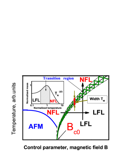
Figure 2: Schematic phase diagram of $\rm YbRh_{2}Si_{2}$ (6) with magnetic field as a control parameter. The vertical and horizontal arrows show LFL-NFL and NFL-LFL transitions at fixed $B$ and $T$ respectively. At $B<B_{c0}$ the system is in AFM state. The width of the transition region $T_{w}\propto T$ is shown by the segment between two vertical arrows. Inset shows a schematic plot of the normalized effective mass versus the normalized temperature. Transition region, where $M^{*}_{N}$ reaches its maximum at $T/T_{\rm max}=1$, is shown by the hatched area both in the main panel and in the inset.

Now we have everything to construct the schematic phase diagram of the HF metal $\rm YbRh_{2}Si_{2}$ at $B\ll B^{*}$. The phase diagram is reported in fig. 2. The magnetic field $B$ plays a role of the control parameter, driving the system towards its QCP. In our case this QCP is of FCQPT type. The FCQPT peculiarity occurs at $B=B_{c0}$, yielding new strongly degenerate state at $B<B_{c0}$. To lift this degeneracy, the system forms either superconducting (SC) or magnetically ordered (ferromagnetic (FM), antiferromagnetic (AFM) etc) states [2]. In the case of $\rm YbRh_{2}Si_{2}$, this state is AFM one [1]. As it follows from eqs. (6) and (7) and seen from fig. 2, at $B\geq B_{c0}$ the system is in either NFL or LFL states. At fixed temperatures the increase of $B$ drives the system along the horizontal arrow from NFL state to LFL one. On the contrary, at fixed magnetic field and raising temperatures the system transits along the vertical arrow from LFL state to NFL one. The inset to fig. 2 demonstrates the behavior of the normalized effective mass $M^{*}_{N}=M^{*}/M^{*}_{\rm max}$ versus normalized temperature $y=T/T_{\rm max}$ following from eq. (6). The $T^{-2/3}$ regime is marked as NFL one since (contrary to LFL case where the effective mass is constant) the effective mass depends strongly on temperature. It is seen that temperature region $y\sim 1$ signifies a transition regime between the LFL behavior with almost constant effective mass and NFL one, given by $T^{-2/3}$ dependence. Thus, temperatures $T\simeq T_{\rm max}$, shown by arrows in the inset and main panel, can be regarded as a transition regime between LFL and NFL states. It is seen from eq. (7) that the width of the transition regime $T_{w}\propto T$ is proportional to $(B-B_{c0})$. It is shown by the segment between two vertical arrows in fig 2. These theoretical results are in good agreement with the experimental facts [1, 7].

Our calculations of the normalized effective mass $M^{*}_{N}(T_{N})$ at fixed high magnetic field $B^{*}$ are shown by the solid line in the main panel of fig. 1. We recollect that in this case the quasiparticles spins are completely polarized. This reveals the above scaling behavior of the normalized experimental curves in terms of the normalized variable $y=T/T_{\rm max}(B)$. It is seen from fig. 1 that our calculations deliver a good description of the experiment [1]. Namely, at elevated temperatures ($y\simeq 1$) the LFL state first converts into the transition one and then disrupts into the NFL state.

To perceive further the behavior of the system at high magnetic fields, in fig. 3 we collect the curves $M^{*}_{N}(T_{N})$ both at low (symbols in the upper box in fig. 3) and high (symbols in the lower box) magnetic fields $B$. All curves have been extracted from the experimental facts [1, 8]. It is seen that while at low fields the low-temperature ends ($T_{N}\sim 0.1$) of the curves completely merge, at high fields this is not the case. Moreover, the low-temperature asymptotic value of $C/T=M^{*}_{N}$ at low fields is around two times more then that at high fields. The physical reason for low-field curves merging is that the effective mass does not depend on spin variable so that the polarizations of subbands with $\sigma_{\uparrow}$ and $\sigma_{\downarrow}$ are almost equal to each other. This is reflected in our calculations, based on eq. (6) for low magnetic fields $B<<B^{*}$. The result is shown by the dotted line in fig. 3.

It is also seen from fig. 3 that all low-temperature differences between high- and low field behavior of the normalized effective mass disappear at high temperatures. In other words, while at low temperatures the values of $M^{*}_{N}$ for low fields are two times more then those for high fields, at temperatures $T_{N}\geq 1$ this difference disappear. It is seen that these high temperatures lie about the transition region, marked by hatched area in the inset to fig. 2. This means that two states (LFL and NFL) separated by the transition region are clearly seen in fig. 3 displaying good agreement between our calculations (dotted line for low fields and thick line at high fields) and the experimental points (symbols).

It is seen from fig. 3, that at high fields $B\sim B^{*}$, (symbols in the lower box) the curves $M^{*}_{N}(T_{N})$ do not merge in the low temperature LFL state. Moreover, their values decrease as $B$ grows representing the full spin polarization of the HF band at the highest reached magnetic fields. This behavior is opposite to that at low fields. The corresponding theoretical curve has been generated from the explicit numerical solution of eq. (5) with respect to eqs. (3) and (4). As we have mentioned above, at temperature raising all effects of spin polarization smear down, yielding the restoration of NFL behavior at $T\simeq\mu_{B}B$. Our high-field calculations (solid line in fig. 3) reflect the latter fact and are also in good agreement with experimental facts. In order not to overload fig. 3 with unnecessary details, we show the calculations only for the case of the complete spin polarization.

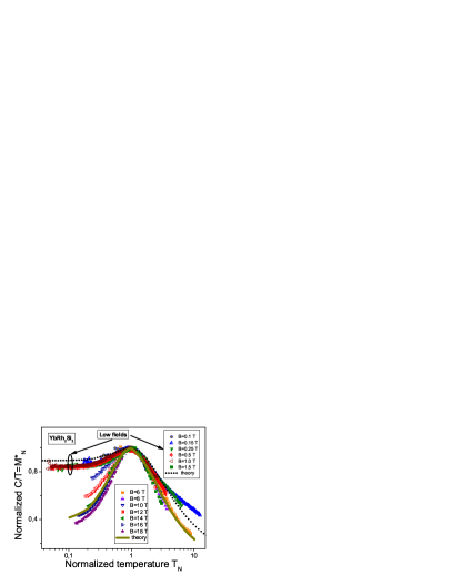
Figure 3: Joint behavior of the normalized effective mass $M^{*}_{N}$ at low (upper box symbols) and high (lower box symbols) magnetic fields extracted from the specific heat ($C/T$) measurements of the $\rm YbRh_{2}Si_{2}$ [8]. Our low-field calculations are depicted by the dotted line tracing the scaling behavior of $M^{*}_{N}$. Our high-field calculations (solid line) are taken at $B\sim B^{*}$ when the quasiparticle band becomes fully polarized.

Figure 4 reports the maxima $M^{*}_{\rm max}(B)$ of the functions in the inset to fig. 1 versus $B$. The solid line represents our approximation for these maxima $M^{*}_{\rm max}(B)\propto 1/\sqrt{B-B_{c0}}$ calculated within the framework of FCQPT theory [9, 2]. It is seen that our calculations are in good agreement with the experimental facts in the entire magnetic field domain. Such good coincidence indicates that at $T\simeq\mu_{B}B$ the transition regime occurs and the NFL behavior restores at high temperatures $T\sim 20$ K.

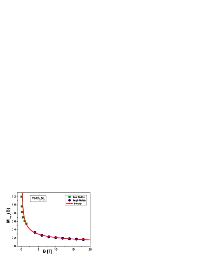
Figure 4: The maxima $M^{*}_{\rm max}(B)$ of the functions $C/T$ versus magnetic field $B$ for $\rm YbRh_{2}Si_{2}$. The points for low [8] (squares) and high fields [1] (circles) are shown in the legend. The solid curve is approximated by $M^{*}_{\rm max}(B)\propto d/\sqrt{B-B_{c0}}$, $d$ is a fitting parameter.

In fig. 5, the solid squares and circles denote temperatures $T_{\rm max}$ at which the maxima of $C/T$ (from the inset to fig. 1) occur. To fit the experimental data [1, 8] the function $T_{\rm max}(B)=b(B-B_{c0})$ defined by eq. (7) with $b\simeq 0.74\,{\rm K/T}$ is used. It is seen from fig. 5 that our calculations (solid line) are in accord with experimental facts, and we conclude that the transition regime of $\rm YbRh_{2}Si_{2}$ is restored at temperatures $T\simeq\mu_{B}B$.

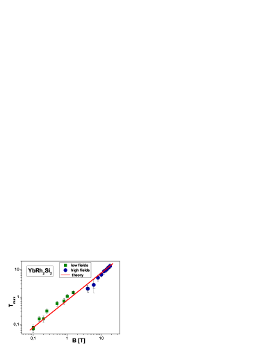
Figure 5: The temperatures $T_{\rm max}(B)$ at which the maxima of $C/T$ in $\rm YbRh_{2}Si_{2}$ (inset to fig. 1) are located. Squares correspond to low-field case [8] and circles to high fields one [1]. The solid line represents the function $T_{\rm max}\propto b(B-B_{c0})$, $b$ is a fitting parameter, see eq. (7).

Consider now the magnetization $M(B,T)$ as a function of magnetic field $B$ at fixed temperature $T$

$$M(B,T)=\int_{0}^{B}\chi(z,T)dz,$$ (8)

where the magnetic susceptibility $\chi$ is given by [3]

$$\chi(B,T)=\frac{\beta M^{*}(B,T)}{1+F_{0}^{a}}.$$ (9)

Here, $\beta$ is a constant and $F_{0}^{a}$ is the spin-antisymmetric Landau amplitude taken at $L=0$.

Our calculations show that the magnetization exhibits a kink at some magnetic field $B=B_{k}$. The experimental magnetization demonstrates the same behavior [11, 10]. We use $B_{k}$ and $M(B_{k})$ to normalize $B$ and $M$ respectively. In the normalized variables, there are no coefficients $\beta$ and $(1+F_{0}^{a})$ so that $\chi\propto M^{*}$ [2] and we can once more use eq. (5) to calculate the magnetic susceptibility $\chi$. The normalized magnetization $M(B)/M(B_{k})$ both extracted from experiment (symbols) and calculated one (solid line), are reported in the inset to fig. 6. It shows that our calculations are in good agreement with the experiment. All the data exhibit the kink (shown by the arrow) at $B_{N}\simeq 1$ taking place as soon as the system enters the transition region. This region corresponds to the magnetic fields where the horizontal arrow in fig. 2 crosses the hatched area. To illuminate the kink position, in the fig. 6 we present the $M(B)$ dependence in logarithmic - logarithmic scale. In that case the straight lines show clearly the change of the slope (power in logarithmic scale) of $M(B)$ at the kink.

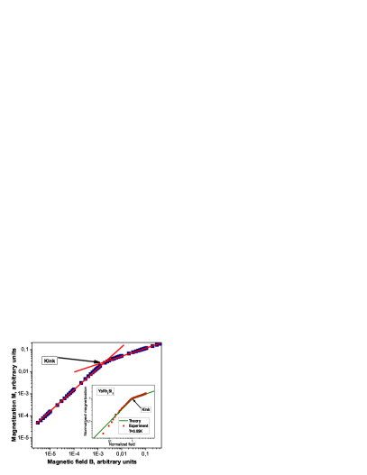
Figure 6: The calculated magnetization $M(B)$ (symbols) and straight lines which are guides for eye. The intersection of the straight lines visualize the kink at the crossover region in the fig. 2. The inset: The field dependencies of the normalized magnetization $M$ of $\rm{YbRu_{2}Si_{2}}$ [10] at $T=0.05$ K. The kink (shown by the arrow) is clearly seen at the normalized field $B_{N}=B/B_{k}\simeq 1$. The solid curve represents our calculations.

At magnetic field $B\simeq B^{*}$ the quasiparticle band becomes fully polarized and a new kink appears [1, 12]. We call this kink as the second one. Our calculations of the normalized magnetization (line) and the experimental points (squares) are shown in fig. 7. In that case both the magnetization and the field are normalized by the corresponding values at the second kink position.

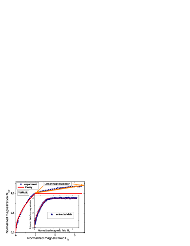
Figure 7: The normalized magnetization $M_{\rm nor}$ as a function of the normalized magnetic field $B_{N}$. Line represents our calculations and squares represent experimental points [1]. The linear dependence $M_{\rm nor}(B_{N})$ is marked by the arrows. The inset demonstrates the experimental data (stars) with the subtracted high-field linear part. Our calculations is shown by the solid line.

In the fig. 7, we plot our theoretical normalized (in the second kink point) magnetization along with experimental one. Good coincidence is seen everywhere except the high-field part at $B_{N}\geq 1$. Here, the experimental normalized magnetization $M_{\rm nor}$ exhibits a linear dependence on $B_{N}$ (marked by two arrows), while the calculated magnetization is approximately constant. Such a behavior is the intrinsic shortcoming of the HF liquid model that accounts for only heavy electrons and omits the conduction electrons of other kind [13, 14]. Thus, we can consider the high-field (at $B_{N}>1$) part of the magnetization as the contribution which is not included in our theory. To separate this contribution from the experimental magnetization curve, we (numerically) differentiate it, then subtract constant part at $B_{N}>1$ and integrate back the resulting curve. The coincidence between our calculations depicted by the solid curve and processed experimental data shown by the stars is reported in the inset to fig. 7. As we can see now, the coincidence between the theory and experiment is good in the entire magnetic field domain. Taking into account the obtained results displayed in figs. 3, 4, 5, 6 and 7, we conclude that the HF system of $\rm{YbRu_{2}Si_{2}}$ evolves continuously under the application of magnetic field. This fact is in agreement with experimental observations [15].

To summarize, here we have analyzed the thermodynamic properties of $\rm YbRh_{2}Si_{2}$ at both low and high magnetic fields. Our calculations allow us to conclude that in magnetic field the HF system of $\rm YbRh_{2}Si_{2}$ evolves continuously without a metamagnetic transition and possible localization of heavy $4f$ electrons. Under the application of magnetic field at low temperatures, the HF system demonstrates the LFL behavior, while at elevated temperatures the system enters the transition region followed by the NFL behavior. Our calculations are in good agreement with experimental facts in the entire temperature and magnetic field domains under consideration.

This work was supported in part by the RFBR grant No. 09-02-00056.

References

- [1] \NameGegenwart P. et al. \REVIEWNew J. Phys.82006171.
- [2] \NameShaginyan V.R., Amusia M.Ya., Msezane A.Z, Popov K.G.\REVIEWPhys. Rep.492201031.
- [3] \NameLandau L.D. \REVIEWSov. Phys. JETP 31956920. \NameLifshitz E. M. Pitaevskii L. P. \BookStatistical Physics, Part 2 \PublButterworth-Heinemann, Oxford \Year1999.
- [4] \NameKhodel V.A., Clark J.W., Zverev M.V. \REVIEWPhys. Rev. B782008075120.
- [5] \NameClark J.W., Khodel V.A. Zverev M.V. \REVIEWPhys. Rev. B712005012401.
- [6] \NameTakahashi D. et al. \REVIEWPhys. Rev. B672003180407(R).
- [7] \NameFriedemann S. et al. \REVIEWProc. Natl. Acad. Sci. USA107201014547.
- [8] \NameOeschler N. et al. \REVIEWPhysica B40320081254.
- [9] \NameShaginyan V.R. \REVIEWJETP Lett.792004286.
- [10] \NameGegenwart P. et al. \REVIEWPhysica B40320081184.
- [11] \NameGegenwart P. et al. \REVIEWScience3152007969.
- [12] \NameKusminskiy S.V., Beach K.S.D., Castro Neto A.H. Campbell D.K. \REVIEWPhys. Rev. B772008094419.
- [13] \NameSaso T. Itoh M. \REVIEWPhys. Rev. B5319966877.
- [14] \NameSatoh H. Ohkawa F. J. \REVIEWPhys. Rev. B632001184401.
- [15] \NameRourke P.M.C. et al. \REVIEWPhys. Rev. Lett.1012008237205.