Negative Binomial Distribution
and the multiplicity moments at the LHC

Abstract

In this work we show that the latest LHC data on multiplicity moments $C_{2}-C_{5}$ are well described by a two-step model in the form of a convolution of the Poisson distribution with energy-dependent source function. For the source function we take $\Gamma$ Negative Binomial Distribution. No unexpected behavior of Negative Binomial Distribution parameter $k$ is found. We give also predictions for the higher energies of 10 and 14 TeV.

One of the widely discussed, yet unsolved, problems in high energy hadron scattering is the production mechanism of low and medium $p_{\text{T}}$ hadrons. Here perturbative QCD cannot be applied and one resorts to phenonemonological models and/or Monte Carlo generators [1]. With the advent of any new hadron accelerator the quantities first studied are charged particle multiplicities. Indeed, the first physics LHC paper, the one by Alice collaboration [2], dealt with the average multiplicity. By now data on multiplicity moments were published by Alice [3] and CMS [4]. It is therefore important to find if their behavior can be explained in terms of some simple phenomenological models or the widely used MC generators. The latter has been recently addressed in Refs.[5].

Throughout this paper we explore the well known observation, recently recalled in Ref.[6], that multiparticle production can be described by the probability distribution $P(n)$ which is a superposition of some unknown distribution of sources $F$, and the Poisson distribution describing particle emission from one source. This is a typical situation in many microscopic models of multiparticle production. For example in Dual Parton Model (DPM) particles are emitted by chains spanned between the colliding protons (for review see Ref.[7]). In that case there are many sources whose number increases with energy. Similarly in Quark-Gluon String Model (QGSM) emission proceeds from $n$ cut-pomerons (Ref.[8] and references therein), and again is assumed to be Poissonian.

Here we refrain from formulating a microscopic multiparticle production model and assume a simple phenomenological formula that captures, however, the above mentioned physics of independent emissions encoded in DPM or QGSM:

$$P(n)={\displaystyle\int\limits_{0}^{\infty}}dt\,F(t)\,e^{-\bar{n}t}\frac{(\bar{n}t)^{n}}{n!}.$$ (1)

Here $t$ is a fraction of the average multiplicity, and $F(t)$ the distribution of sources that contribute fraction $t$ to the multiplicity probability $P(n)$. Normalization conditions require

$${\displaystyle\int\limits_{0}^{\infty}}dt\,F(t)={\displaystyle\int\limits_{0}^{\infty}}dt\,t\,F(t)=1.$$ (2)

There are two useful properties of Eq.(1) that will be of importance throughout this paper. The first one is the fact that factorial moments of multiplicity distribution measure directly the $F_{m+1}$ moments of the source:

$$\left\langle n(n-1)(n-2)\ldots(n-m)\right\rangle=\bar{n}^{m+1}{\displaystyle\int\limits_{0}^{\infty}}dt\,t^{m+1}F(t)=\bar{n}^{m+1}F_{m+1}.$$ (3)

Because of (2) average multiplicity

$$\left\langle n\right\rangle=\bar{n}.$$ (4)

Factorial moments can be expressed through scaled regular moments

$$C_{m}=\frac{\left\langle n^{m}\right\rangle}{\left\langle n\right\rangle^{m}}$$ (5)

that have been measured at the LHC [3, 4]. For the first five moments we have:

$$C_{2} =\frac{1}{\left\langle n\right\rangle}+F_{2},$$

$$C_{3} =3\frac{C_{2}}{\left\langle n\right\rangle}-2\frac{1}{\left\langle n\right\rangle^{2}}+F_{3},$$

$$C_{4} =6\frac{C_{3}}{\left\langle n\right\rangle}-11\frac{C_{2}}{\left\langle n\right\rangle^{2}}+6\frac{1}{\left\langle n\right\rangle^{3}}+F_{4},$$

$$C_{5} =10\frac{C_{4}}{\left\langle n\right\rangle}-35\frac{C_{3}}{\left\langle n\right\rangle^{2}}+50\frac{C_{2}}{\left\langle n\right\rangle^{3}}-24\frac{1}{\left\langle n\right\rangle^{4}}+F_{5}.$$ (6)

The second property of Eq.(1) is that for large multiplicities (i.e. for large energies) it implies an approximate KNO (Koba, Nielsen and Olesen) scaling [9]. Indeed, in the limit $\bar{n}\rightarrow\infty$ and fixed $n/\bar{n}$ one can apply the saddle point approximation to calculate $dt$ integral in (1) leading to [6]

$$\psi\equiv\bar{n}P(n)\simeq F\left(\frac{n}{\bar{n}}\right).$$ (7)

KNO scaling says that function $\psi$ depends only on $\tau=n/\bar{n}$.

KNO scaling is seen approximately in the multiplicity distributions measured at SPS and higher energies (see for review [10]) including the LHC [3, 4]. This fact gives strong justification for formula (1) which also allows to give definite predictions for the violation of the KNO scaling. Originally KNO scaling has been derived assuming Feynman scaling [11], which states that the central rapidity density saturates at asymptotic energies. The latter is clearly not seen in the data (e.g. [2]), on the contrary central rapidity density grows as a power of energy. For example for $\left|\eta\right|<0.5$ [12]:

$$\left.\frac{dn}{d\eta}\right|_{\left|\eta\right|<0.5}\sim 0.755\left(\frac{W}{1\,\text{GeV}}\right)^{0.23}$$ (8)

where $W=\sqrt{s}$. For constant $\bar{n}$ all multiplicity moments would be constant as well.

Here we see the advantage of the convolution model (1) since it implies approximate KNO scaling also for energy dependent $\bar{n}$. This energy dependence introduces in turn energy dependence of the moments, as clearly seen from equations (6), even if function $F$ is energy independent. Unfortunately this dependence alone would contradict the data since for constant $F_{n}$ multiplicity moments decrease with energy (for growing $\left\langle n\right\rangle$).

Therefore the source function $F$ has to depend on energy and its moments have to win over the decrease generated by the multiplicity growth through Eqs.(6). In Ref.[6] the method of recovering $F$ from the data has been discussed, without, however, reference to the recent measurements at the LHC. In DPM or QGSM violation of the KNO scaling proceeds by an increase of the number of sources (chains, pomerons) with increasing energy.

Here, rather than constructing a microscopic model of multiparticle production, we choose the explicit form of $F(t)$ and check whether we are able to describe multiplicity moments measured by Alice and CMS. To this end we choose for $F$ negative binomial distribution (NBD) [10]:

$$F(t,k)=\frac{k^{k}}{\Gamma(k)}t^{k-1}e^{-kt}$$ (9)

which is known to describe relatively well the data at lower energies [1]. Distribution (9) depends on one parameter $k$, which – as explained above – has to depend on $W$. It is known from the analysis of lower energy data that, depending on energy, $k\sim 4$ - 2 and decreases with increasing energy. Let us remind that for $k=1$ the probability distribution $P_{\text{NBD}}$ is given by geometrical distribution $P(n)=\left\langle n\right\rangle^{n}/(1+\left\langle n\right\rangle)^{n+1}$. With increasing $k$ ($1/k\rightarrow 0$), the distribution $P_{\text{NBD}}$ is getting narrower tending to the Poisson distribution.

Based on experimental evidence of the wide occurrence of NBD, several possible explanations have been proposed in the literature (for review see Ref.[1]). The NBD has been mostly interpreted in terms of (partial) stimulated emissions or cascade processes [13]. More recently NBD has been derived from the Color Glass Condensate (CGC) approach giving explicit prediction for the energy dependence of parameter $k$ at high energies being of the order of the LHC energy range [14]. Here, contrary to the lower energy trend, parameter $k$ is expected to grow with energy, as it is directly connected to the saturation scale which increases with energy. Similar behavior is found in String Percolation Model (SPM) [15], where – once percolation is achieved – $k$ starts to grow with energy like in the CGC. It is therefore interesting to see if the new regime of growing $k$ has been already achieved at the LHC, which is one of the motivations behind the present work.

For negative binomials

$$F_{m+1}=\frac{k(k+1)\ldots(k+m)}{k^{m+1}}.$$ (10)

The first equation of (6) gives:

$$C_{2}=\frac{1}{\left\langle n\right\rangle}+1+\frac{1}{k}\quad\rightarrow\quad\frac{1}{k}=C_{2}-1-\frac{1}{\left\langle n\right\rangle}.$$ (11)

Using (11) we get for higher moments

$$C_{3} =C_{2}(2C_{2}-1)-\frac{C_{2}-1}{\left\langle n\right\rangle},$$

$$C_{4} =C_{2}(6C_{2}^{2}-7C_{2}+2)-2\frac{3C_{2}^{2}-4C_{2}+1}{\left\langle n\right\rangle}+\frac{C_{2}-1}{\left\langle n\right\rangle^{2}},$$

$$C_{5} =C_{2}(24C_{2}^{3}-46C_{2}^{2}+29C_{2}-6)-2\frac{18C_{2}^{3}-34C_{2}^{2}+19C_{2}-3}{\left\langle n\right\rangle}$$

$$+\frac{14C_{2}^{2}-23C_{2}+9}{\left\langle n\right\rangle^{2}}-\frac{C_{2}-1}{\left\langle n\right\rangle^{3}}.$$ (12)

Let us first observe that for constant $C_{2}$, which is approximately true, at least for $\left|\eta\right|<0.5$ where $C_{2}\simeq 2$, higher moments grow with energy. This is depicted in Fig.1 where long dash (red) line corresponds to constant $C_{2}$ in two rapidity intervals $\left|\eta\right|<0.5$ ($C_{2}\simeq 2$) and $\left|\eta\right|<2.4$ ($C_{2}\simeq 1.54$). It is clearly seen that for negative binomial distribution used here this growth is, however, too slow. For larger rapidity intervals $\Delta\eta$ multiplicity is also larger $dn/d\eta=0.755\,\Delta\eta\,W^{0.23}$ and therefore the inverse powers of multiplicity are less important than for smaller rapidity ranges. Moreover for $\left|\eta\right|<2.4$ second moment $C_{2}\simeq 1.54$ and therefore the coefficients in front of powers $\left\langle n\right\rangle^{-m}$ are also smaller than for $\left|\eta\right|<0.5$. Therefore, as seen in Fig.1, for $\left|\eta\right|<2.4$ in the fit where $C_{2}=$const., all other moments are nearly constant as well.

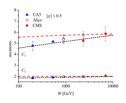
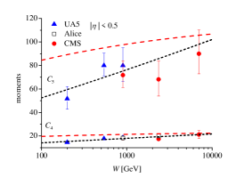
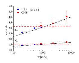
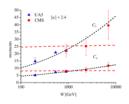
Figure 1: Multiplicity moments measured by UA5 [16], Alice [3] and CMS [4] for two rapidity intervals in function of energy $W=\sqrt{s}$. Long dash (red) lines correspond to constant $C_{2}$ moments equal to 2 and 1.54 for two rapidity intervals $|\eta|<0.5$ and $|\eta|<2.4$ respectively. Short dash (black) lines correspond to energy dependent $C_{2}$ as explained in the text.

Fig.	$\left|\eta\right|<\eta_{0}$	$a$	$b$
1	$0.5$	$1.702$	$0.071$
1	$2.4$	$0.997$	$0.175$
3	$0.5$	$1.597$	$0.111$
3	$1.0$	$1.377$	$0.118$
3	$1.3$	$1.219$	$0.149$

Table 1: Values of parameters $a$ and $b$ of Eq.(13) used in Figs.1 and 3.

In order to reproduce the growth seen in the data we have therefore to require a mild increase of $C_{2}$ with $W$. Higher moments $C_{m}$ are proportional to higher powers of $C_{2}^{m}$ and should therefore grow faster with $W$ with increasing $m$. This trend is clearly seen in the data. To this end we choose to approximate $C_{2}$ by a linear function of $\log W$:

$$C_{2}=a+b\log(W\text{[GeV]}).$$ (13)

In order to find parameters $a$ and $b$ we choose to fit $C_{4}$ rather than $C_{2}$. In both cases $\left|\eta\right|<0.5$ and $\left|\eta\right|<2.4$ moment $C_{4}$ grows rather fast with $W$ having still reasonable errors. Fitting $C_{2}$ gives usually too slow increase of higher moments, whereas fitting $C_{4}$ reproduces all moments with good precision. This is easily seen from Fig.1. The parameters of the fit (13) are given in Table 1 and the resulting energy dependence of $1/k$ is plotted in Fig. 2. We see that the trend from lower energies continues: $k$ decreases with energy but is still rather far from $k=1$. For $\eta<0.5$ and $W=0.9$, 7 and 14 TeV, $k=1.58$, 1.25 and 1.18 respectively. Should this dependence continue, $k=1$ would be reached for $W\sim 250$ TeV. On the other hand dependence of $k$ on rapidity is quite pronounced.

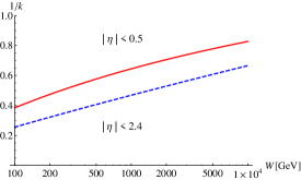
Figure 2: Growth of $1/k$ used in Fig.1.

With parametrizations (8) and (13) we are able to predict the first moments for higher energies at which the LHC will be running in the future. The results are displayed in Table 2.

$W$ [TeV]	10	14	10	14
	$|\eta|<0.5$		$|\eta|<2.4$
$\left\langle n\right\rangle$	6.28	6.78	31.61	34.15
$C_{2}$	1.98	1.99	1.70	1.72
$C_{3}$	5.73	5.81	4.03	4.18
$C_{4}$	21.74	22.30	12.33	13.11
$C_{5}$	102.11	106.02	46.07	50.39

Table 2: Predictions for multiplicity moments.

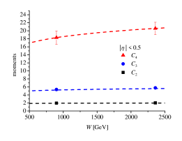
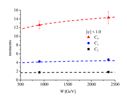
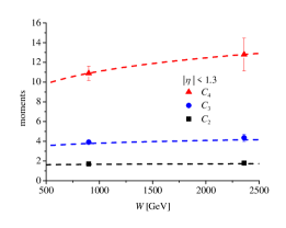
Figure 3: Multiplicity moments in different rapidity intervals as measured by Alice [3] together with NBD fit with $C_{2}$ parametrized as in Eq.(13) and Table 1.

Alice collaboration published results for the multiplicity moments $C_{2}-C_{4}$ for two energies: 0.9 and 7 TeV and three rapidity intervals $|\eta|<0.5$, 1 and 1.3. We repeated the same procedure described above for the Alice data fitting $C_{4}$ with the help of Eq.(13). The resulting parameters are collected in Table 1 and the moments are plotted in Fig.3. We see good agreement of NBD fits for all three rapidity intervals.

To conclude: we have used the convolution model (1) with distribution of sources given by negative binomial function (9) to fit multiplicity moments measured recently by Alice and CMS collaborations at the LHC. We have shown that convolution model implies that normalized $C_{m}$ multiplicity moments decrease with increasing energy as inverse powers of the average multiplicity (11,12) if the distribution function $F(t)$ is energy independent. Such a behavior contradicts data. Assuming NBD for $F(t)$ and logarithmic growth (13) of $C_{2}$ moment, we have been able to reproduce the multiplicity moments over the wide range of energies for different rapidity intervals. The input growth of $C_{2}$ with energy can be easily translated to a decrease of the parameter $k$ of NBD function (9). This behavior is consistent with lower energies and does not exhibit the change predicted by CGC [14] and/or SPM [15]. We also made predictions for higher energies which will be soon accessible at the LHC. Unfortunately we are still lacking a microscopic model explaining energy dependence of $k$ parameter of the NBD distribution.

Acknowledgments: I am grateful to Andrzej Bialas for discussions that triggered this research and for reading the manuscript. Also discussions with Krzysztof Fialkowski were of considerable help. Comments by Carlos Pajares and Elena Kokoulina are also acknowledged.

References

- [1] For a review see: W. Kittel, E.A. De Wolf, Soft Multihadron Dynamics, World Scientific, 2005.
- [2] KAamodt et al. [ ALICE Collaboration ], Eur. Phys. J. C65 (2010) 111-125, [arXiv:0911.5430 [hep-ex]].
- [3] K. Aamodt et al. [ ALICE Collaboration ], Eur. Phys. J. C68 (2010) 89-108, [arXiv:1004.3034 [hep-ex]].
- [4] V. Khachatryan et al. [ CMS Collaboration ], [arXiv:1011.5531 [hep-ex]].
- [5] K. Fialkowski, R. Wit, Eur. Phys. J. C70 (2010) 1-4, [arXiv:1006.5800 [hep-ph]] and Acta Phys. Polon. B42 (2011) 293-306, [arXiv:1012.4922 [hep-ph]].
- [6] A. Bialas, Acta Phys. Polon. B41 (2010) 2163-2174.
- [7] A. Capella, U. Sukhatme, C-I. Tan, J. Tran Thanh Van, Phys. Rept. 236 (1994) 225-329.
- [8] A. B. Kaidalov, M. G. Poghosyan, Eur. Phys. J. C67 (2010) 397-404. [arXiv:0910.2050 [hep-ph]].
- [9] Z. Koba, H. B. Nielsen, P. Olesen, Nucl. Phys. B40 (1972) 317-334.
- [10] J. F. Grosse-Oetringhaus, K. Reygers, J. Phys. G G37 (2010) 083001, [arXiv:0912.0023 [hep-ex]].
- [11] R. P. Feynman, Phys. Rev. Lett. 23 (1969) 1415-1417.
- [12] L. McLerran, M. Praszalowicz, Acta Phys. Polon. B41 (2010) 1917-1926, [arXiv:1006.4293 [hep-ph]] and Acta Phys. Polon. B42 (2010) 99, [arXiv:1011.3403 [hep-ph]].
- [13] A. Giovannini, L. Van Hove, Z. Phys. C30 (1986) 391.
- [14] F. Gelis, T. Lappi, L. McLerran, Nucl. Phys. A828 (2009) 149-160. [arXiv:0905.3234 [hep-ph]].
- [15] J. Dias de Deus, C. Pajares, Phys. Lett. B695 (2011) 211-213. [arXiv:1011.1099 [hep-ph]].
- [16] G. J. Alner et al. [ UA5 Collaboration ], Phys. Lett. B160 (1985) 193.