Swapping and entangling hyperfine coupled nuclear spin baths

Abstract

We numerically study the hyperfine induced nuclear spin dynamics in a system of two coupled quantum dots in zero magnetic field. Each of the electron spins is considered to interact with an individual bath of nuclear spins via homogeneous coupling constants (all coupling coefficients being equal). In order to lower the dimension of the problem, the two baths are approximated by two single long spins. We demonstrate that the hyperfine interaction enables to utilize the nuclear baths for quantum information purposes. In particular, we show that it is possible to swap the nuclear ensembles on time scales of seconds and indicate that it might even be possible to fully entangle them. As a key result, it turns out that the larger the baths are, the more useful they become as a resource of quantum information. Interestingly, the nuclear spin dynamics strongly benefits from combining two quantum dots of different geometry to a double dot set up.

Introduction.–Electron spins confined in semiconductor quantum dots with an s-type conduction band, like for example GaAs quantum dots, experience decoherence through the spin-orbit interaction, and by the hyperfine interaction with surrounding nuclear spins. With respect to possible future solid state quantum computation systems utilizing the electron spin as the qubit LossDi98 ; Hanson07 , these interactions act as a source of decoherence. Due to the spatial confinement of the electron spin in a quantum dot, the relaxation time $T_{1}$ induced by the spin-orbit interaction is enhanced for low temperatures KhaNaz00 ; KhaNaz01 . As the dephasing time $T_{2}$ due to the spin orbit interaction turns out to be as long as the $T_{1}$ time under realistic conditions GolKhaLoss04 , the major source of decoherence in semiconductor quantum dots results from the hyperfine interaction KhaLossGla02 ; KhaLossGla03 ; Petta05 ; Koppens06 ; Braun05 . For related reviews the reader is referred to Refs. SKhaLoss03 ; Zhang07 ; Klauser07 ; Coish09 ; Taylor07 . Similar situations arise in carbon nanotube quantum dots Church09 , phosphorus donors in silicon Abe04 and nitrogen vacancies in diamond Jel04 ; Child06 ; Hanson08 .

Apart from this detrimental effect of the hyperfine interaction, it provides a way to efficiently access the nuclear spins by e.g. external degrees of freedom. This for example enables to built up an interface between light and nuclear spins SchCiGi08 ; SchCiGi09 , to polarize nuclear spin baths Taylor03 ; ChriCiGi09 ; ChriCiGi07 , to set up long-lived quantum Taylor032 ; Morton08 and classical Austing09 memory devices or to generate entanglement ChriCiGi08 .

In both of the aforementioned contexts it is of key importance to understand the hyperfine induced spin dynamics. Here one has to distinguish between the case of a strong and the case of a weak magnetic field applied to the electron spins. In the first limit, the “flip-flop” terms between the electron and the nuclear spins occurring in the Hamiltonian are strongly suppressed. This allows to treat them perturbatively or to even completely neglect them, which strongly simplifies the calculations KhaLossGla02 ; KhaLossGla03 ; Coish04 ; Coish05 ; Coish06 ; Coish08 . In the absence of such an external magnetic field, however, many approximative techniques break down, and one has to resort to exact methods. As explained in Ref. ErbSchl09 , in order to gain exact results, strong restrictions on the initial state KhaLossGla02 ; KhaLossGla03 , the size of the system SKhaLoss02 ; SKhaLoss03 or the hyperfine coupling constants BorSt07 ; ErbS09 ; ErbSchl09 ; ErbSchl10 have to be made.

In the present paper we combine the second and the third approach and focus on the advantages of the hyperfine interaction. To this end we consider a model of two exchange coupled electron spins each of which is interacting with an individual bath of nuclear spins. This corresponds to the situation of spatially well-separated quantum dots. Assuming the baths to be strongly polarized in opposite directions initially, we investigate, by means of exact numerical diagonalization, to what extent it is possible to swap and entangle them. Usually exact numerical diagonalizations are restricted to rather small system sizes. In order to go beyond these limits, we reduce the dimension of the problem by approximating the two baths by two single long spins. The spectral properties of the model described above have recently been studied in Ref. ErbSchl10 , where it has been shown that the spectrum of the Hamiltonian exhibits systematically degenerate multiplets. Motivated by these findings, below we will distinguish between an inversion symmetric system, showing the mentioned degeneracies, and a system with broken inversion symmetry where such degeneracies are absent.

The work presented in this paper complements the results of Ref. ErbSchl09 , where we analytically studied the homogeneous coupling case for two electron spins coupled to a common bath of nuclear spins. Choosing the hyperfine coupling constants to be equal to each other of course has to be regarded as a rough approximation. However, it has been shown that already such simple models can yield concrete predictions and realistic results ErbSchl09 ; SchCiGi08 ; SchCiGi09 ; ChriCiGi09 ; ChriCiGi08 .

Model and methods.–The Hamiltonian of two exchange coupled electron spins, each of which is interacting with an individual bath of nuclear spins via the hyperfine interaction reads

$$H=\vec{S}_{1}\cdot\sum_{i=1}^{N_{1}}A_{i}^{1}\vec{I}_{i1}+\vec{S}_{2}\cdot\sum_{i=1}^{N_{2}}A_{i}^{2}\vec{I}_{i2}+J_{ex}\vec{S}_{1}\cdot\vec{S}_{2},$$ (1)

where $\vec{S}_{j}$ are the electron and $\vec{I}_{ij}$ are the nuclear spins the $j$-th electron spin interacts with. For simplicity we will consider $N_{1}=N_{2}=:N$ in what follows. The parameter $J_{ex}$ denotes an exchange coupling between the two electron spins, which can experimentally be adjusted in a range of $[-10^{-3},10^{-3}]$eV, and $A_{i}^{1}$, $A_{i}^{2}$ are the hyperfine coupling constants. In a realistic quantum dot these are proportional to the square modulus of the electronic wave function at the sites of the surrounding nuclear spins. As a typical example, in GaAs quantum dots the overall coupling strength of the $j$-th electron spin $A^{j}:=\sum_{i=1}^{N}A_{i}^{j}$ is of the order of $\left[10^{-4},10^{-5}\right]$eV.

Due to the spatial variation of the electronic wave function, the hyperfine couplings are clearly inhomogeneous. However, in the following we consider them to be equal to each other, meaning that $A^{j}_{i}=A^{j}/N$. Then the Hamiltonian (1) conserves apart from the total spin $\vec{J}=\vec{S}_{1}+\vec{S}_{2}+\vec{I}_{1}+\vec{I}_{2}$, where $\vec{I}_{j}=\sum_{i=1}^{N_{j}}\vec{I}_{ij}$, also the squares of the total bath spins $\vec{I}^{2}_{j}$

$$\left[H,\vec{J}\right]=\left[H,\vec{I}_{j}^{2}\right]=0.$$ (2)

The first symmetry will be helpful for the exact numerical diagonalizations of the Hamiltonian matrix SKhaLoss02 ; SKhaLoss03 , through which we will obtain the dynamics in the following. We compute the time dependent density matrix by decomposing the initial state into energy eigenstates and applying the time evolution operator. Tracing out the electron degrees of freedom then yields the reduced density matrix of the nuclear baths $\rho_{n}(t)$ from which we can calculate the time evolution of all observables. For details the reader is referred to Ref. ErbSchl09 .

In the following we will approximate each of the two baths $\vec{I}_{j}$ by a single long spin. Let us briefly discuss to which physical situation this corresponds. A general state of a bath is a superposition of states from different multiplets

$$\lvert\beta_{j}\rangle=\sum_{I_{j},m_{j}}\beta_{j}^{I_{j},m_{j}}\lvert I_{j},m_{j}\rangle,$$ (3)

where the quantum numbers associated with a certain Clebsch-Gordan decomposition of the bath have been omitted. The number of multiplets contributing to the sum in (3) decreases with increasing bath polarization. For very high polarizations we can therefore approximate the state (3) by $\lvert\beta_{j}\rangle=\lvert I,m_{j}\rangle$ with $m_{j}\approx\pm I$. Due to the commutation relations (2) all dynamics is then captured by the following simple Hamiltonian, to which we refer to as the long spin approximation Hamiltonian:

$$H_{\text{LSA}}=\frac{A^{1}}{2I}\vec{S}_{1}\cdot\vec{I}_{1}+\frac{A^{2}}{2I}\vec{S}_{2}\cdot\vec{I}_{2}+J_{ex}\vec{S}_{1}\cdot\vec{S}_{2}$$ (4)

The form of the couplings $A^{j}/2I$ results from the observation that the $N$ bath spins can couple to $I=N/2,N/2-1,N/2-2,\ldots$. As we assume highly polarized baths, we consider the maximal value $I=N/2$. Solving for $N$ then yields the coupling constants in (4). For later convenience we define $A:=A^{1}+A^{2}$.

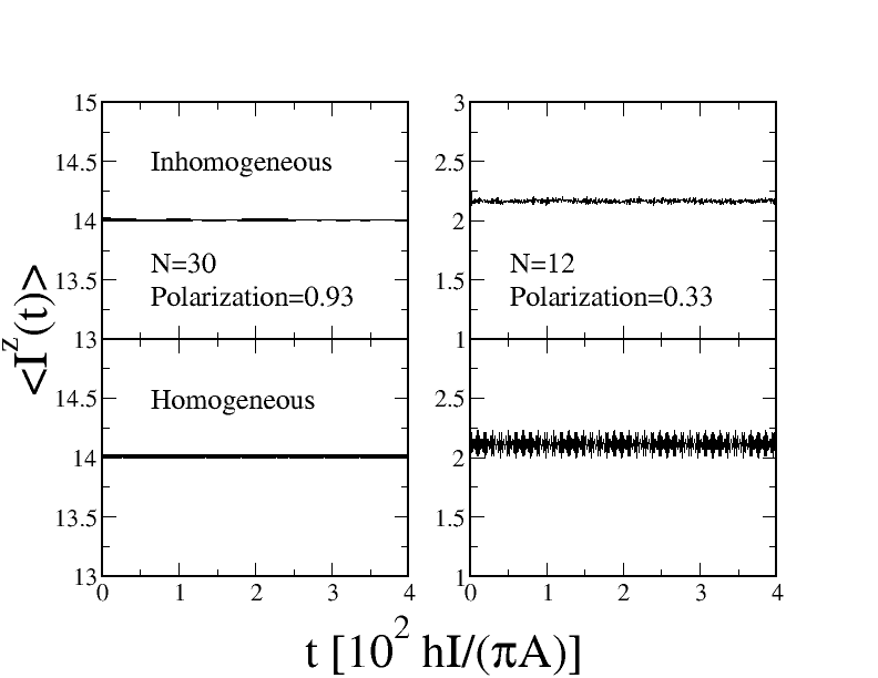
Figure 1: Nuclear spin dynamics of the Gaudin model for inhomogeneous (upper panels) and homogeneous (lower panels) hyperfine couplings. The bath state is initially randomly correlated SKhaLoss02 ; SKhaLoss03 and the electron spin is pointing upwards. The left column shows the case of $N=30$ and a bath polarization of $0.93$, while in the right column we have $N=12$ and a polarization of $0.33$. Even in the latter case the bath dynamics for inhomogeneous and homogeneous couplings are still quite similar to each other.

High nuclear polarizations of up to $80\%$ have been experimentally demonstrated in Refs. Atac ; Ono ; Baugh ; Tarucha . In particular, Ref. Tarucha also discussed the possibility of polarizing two nuclear ensembles in different directions. However, a question concerning the LSA arises from assuming the couplings to be homogeneous: As demonstrated in Ref. ErbSchl09 , this approximation is a good one for short time scales, whereas for longer times artifacts occur. As the nuclear dynamics are slow, it has to be questioned to what extent homogeneous couplings are adequate in order to evaluate nuclear spin dynamics. Therefore we numerically investigated the time evolution of the nuclear spins in the Gaudin model. The Gaudin model is the central spin model with a single central spins, as corresponding to one of the two first terms in the Hamiltonian (1). As a result from our numerics, we find that the influence of inhomogeneities is suppressed with increasing polarization. This is illustrated Fig. 1 where we compare cases of high and low polarization. Even in the latter case the dynamics for both types of couplings are very close to each other. In the LSA we are considering two coupled Gaudin models. Consequently, the data presented in Fig. 1 does not give a strict proof for the adequacy of neglecting inhomogeneities in the couplings. However, it clearly provides qualitative evidence into this direction.

Swapping nuclear spin polarizations.–We will now evaluate the nuclear spin dynamics within the LSA and explore the possibility of swapping oppositely polarized spin baths, $\langle I_{1}^{z}\rangle=-\langle I_{2}^{z}\rangle$. Our initial state $\lvert\alpha\rangle$ will be a simple product state between the electron and the nuclear state $\lvert\alpha\rangle=\lvert\alpha_{e}\rangle\lvert\alpha_{n}\rangle$. Since both baths are spatially well-separated, the initial nuclear state is again a product state of the two long spins. Note that entanglement within the baths can not be considered within the LSA. However, due to their high polarizations, correlations within the baths are of minor importance. In what follows, we will always work in subspaces of fixed $J^{z}=:M$ where only the $z$-component has a non-zero expectation value $\langle I_{j}^{z}(t)\rangle$. Note that (again) due to the high bath polarizations, it is realistic to assume that the initial state has components exclusively in subspaces of fixed $M$. Moreover, we will assume the $z$-component of the total electron spin to be initially zero, i.e. the spins are antiparallel. Similar results as to be presented below are obtained for more general initial states of the electron spin system.

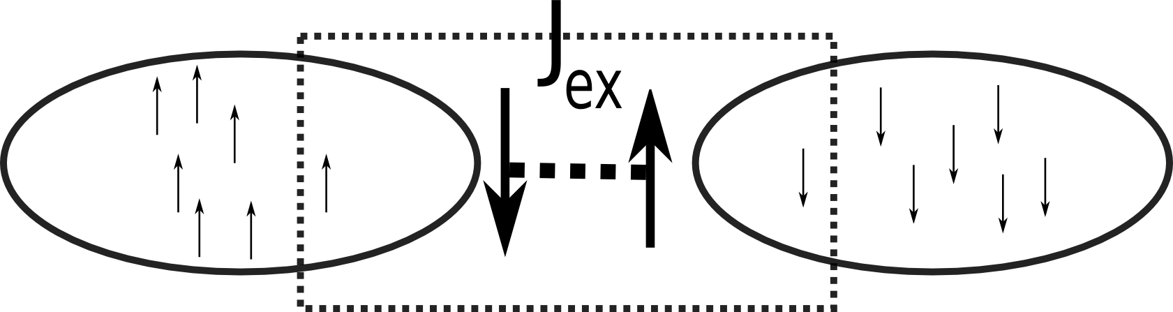
Figure 2: The nuclear baths are considered to consist of spins with length $(1/2)$. The frame marks the LSA system with the smallest possible bath spin length $I=1/2$. Here the dynamics of all four spins are highly coherent provided the values of all couplings are close to each other, motivating the condition (5) (see text).

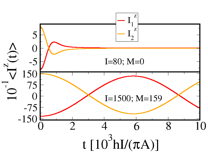
Figure 3: Nuclear spin dynamics for $J_{ex}/(A/2I)=3.5$, $\Delta=0$ and $\lvert\alpha\rangle=(1/\sqrt{13})\left(2\lvert\Uparrow\Downarrow\rangle+3\lvert\Downarrow\Uparrow\rangle\right)\lvert M-I,I\rangle$. The upper panel shows data data $I=80$ and $M=0$ where the expectation values $\langle I_{j}^{z}(t)\rangle$ decay rapidly to zero. In the bottom panel we consider $I=1500$ and $M=159$ where an almost complete swap of the nuclear spins is observed.

More importantly, we will concentrate on exchange couplings being of the same order of magnitude as the hyperfine coupling strength,

$$J_{ex}/(A/2I)\approx 1,$$ (5)

meaning that the two electron spins are coupled as strongly to each other as they are coupled to the bath spins. This is motivated by the following observation. Let us consider (4) for the smallest possible value, $I=1/2$. As shown by elementary numerics, the dynamics of all four spins are, under the condition (5), highly coherent, and the nuclear spin polarizations can nicely be swapped, i.e. at the end of the process the expectation values $\langle I_{j}^{z}(t)\rangle$ are, to a very good degree of accuracy, exchanged as compared to the initial state. Let us now consider the two baths in the original model (1) to consist of spins with length $(1/2)$, as already assumed for the derivation of the couplings in (4). As depicted in Fig. 2, the complete system can now be regarded as set of $I=1/2$ models. Thus, from a heuristic point of view, the biggest chance to swap the full baths exists if all the subsystems are swapped. Hence, the exchange coupling has to be of the order of the coupling between the electron and the bath spins for any subsystem. For homogeneous couplings within the baths, this means that $J_{ex}\approx A/N$, which translates into (5) for the LSA, as explained above.

However, at first sight, it does not seem to be possible to swap the initially antiparallel nuclear spins $I>1/2$, even if the condition (5) is fulfilled. This is demonstrated in the upper panel of Fig. 3, where we consider $I=80$, $J_{ex}/(A/2I)=3.5$ and a zero “detuning” $\Delta:=A_{2}-A_{1}=0$. This corresponds to a situation in which the two quantum dots have the same geometries. We choose the comparatively generic electron spin state $\lvert\alpha_{e}\rangle=(1/\sqrt{13})\left(2\lvert\Uparrow\Downarrow\rangle+3\lvert\Downarrow\Uparrow\rangle\right)$ (similar results occur for other choices) and plot the dynamics for antiparallel nuclear spin configurations with the maximal possible $z$ components $\lvert\alpha_{n}\rangle=\lvert-I,I\rangle$. As seen from the figure, the expectation values of the bath spins decrease quite rapidly to zero and are far away from being properly swapped.

Surprisingly, this apparently negative result turns out to be related to the size of the baths in the following sense: Consider an initial state with the electron spins being in an arbitrary linear combination of $\lvert\Uparrow\Downarrow\rangle$, $\lvert\Downarrow\Uparrow\rangle$ and a nuclear state $\lvert I_{1}^{z},I_{2}^{z}\rangle$ fulfilling, say, $I_{1}^{z}<0$ and $I_{2}^{z}>0$ with $|I_{1}^{z}|<|I_{2}^{z}|$, i.e. the “magnetization” $M_{r}:=M/(2I+1)$ is nonzero, $M_{r}=(|I_{2}^{z}|-|I_{1}^{z}|)/(2I+1)\neq 0$. Here we find that for magnetizations larger than a certain “critical” value $M_{r}^{c}$ (slightly depending on the electron spin state) the expectation value $\langle I_{1}^{z}(t=0)\rangle$ is, to a an excellent degree of accuracy, completely reversed. As a representative example, in the left panel of Fig. 4 we plot the quantity $\langle I_{1}^{z}(t)\rangle$ for $I=200$ with, as before, $\lvert\alpha_{e}\rangle=(1/\sqrt{13})\left(2\lvert\Uparrow\Downarrow\rangle+3\lvert\Downarrow\Uparrow\rangle\right)$ as initial electron spin state. We consider two different initial nuclear states $\lvert\alpha_{n}\rangle=\lvert M-I,I\rangle$, where the corresponding value of $M_{r}$ is in one case exactly at, in the other case lower than the critical $M_{r}^{c}$ at the given nuclear spin length. In the latter case the reversal of $\langle I_{1}^{z}(t)\rangle$ is slightly incomplete.

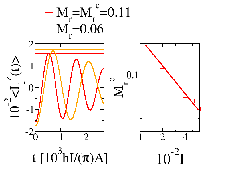
Figure 4: Left panel: $\langle I_{1}^{z}(t)\rangle$ for $J_{ex}/(A/2I)=3.5$, $\Delta=0$ and $I=200$. The initial state is $\lvert\alpha\rangle=(1/\sqrt{13})\left(2\lvert\Uparrow\Downarrow\rangle+3\lvert\Downarrow\Uparrow\rangle\right)\lvert M-I,I\rangle$ where two values of the magnetization $M_{r}=M/(2I+1)$ are considered; $M_{r}=M_{r}^{c}=0.11$ corresponds to the critical value at $I=200$. The horizontal lines are guides to the eye indicating the value needed for a complete reversal of $\langle I_{1}^{z}(t)\rangle$. Right panel: $M_{r}^{c}$ versus spin length $I$ for the same initial state as in the left panel: The fit results in a power-law decrease $M_{r}^{c}(I)=e^{-0.5}I^{-0.33}$. Thus, for large enough spin baths antiparallel nuclear spin configurations can, to an excellent degree of accuracy, be swapped.

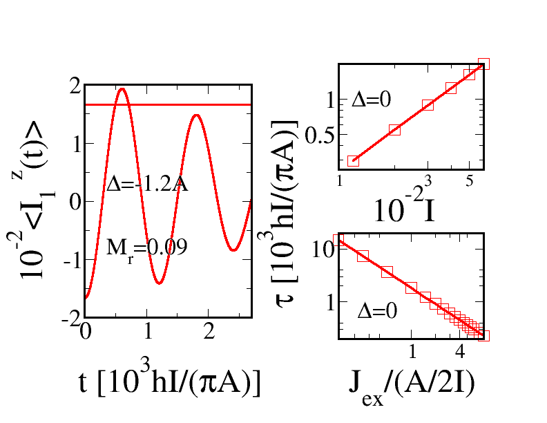
Figure 5: Left panel: Reversal of $\langle I_{1}^{z}(t)\rangle$ for the same situation as in Fig. 4 left panel, but $\Delta=-1.2A$ and $M_{r}=0.09$: Breaking inversion symmetry facilitates swapping the nuclear spin polarizations. Right panels: Swap time $\tau$ at $\Delta=0$ and $J_{ex}/(A/2I)=3.5$ as a function of $I$ (upper panel), and at $I=200$ as a function of $(J_{ex}/(A/2I))$ (lower panel). In the upper case we find a power law as $\tau=e^{0.015}I^{1.19}\left(hI/\pi A\right)$, in the lower case $\tau=e^{7.51}\left[J_{ex}/(A/2I)\right]^{-1.003}\left(hI/\pi A\right)$.

It is now a key observation that $M_{r}^{c}(I)$ strongly decreases with increasing spin length $I$. This is demonstrated in the right panel of Fig. 4 for spin lengths up to $I=600$, where a clear power law scaling is found:

$$M_{r}^{c}\approx e^{-\frac{1}{2}}\cdot I^{-\frac{1}{3}}$$ (6)

Hence, for a large enough value of $I$ the magnetization $M_{r}^{c}$ will be so close to zero that, up to irrelevant corrections, antiparallel nuclear spin configurations can indeed be swapped. To give a quantitative example, for $I=10^{6}$ (as typical for the nuclear spin bath of GaAs quantum dots) the above power law leads to $M_{r}^{c}=0.006$ implying that baths with $I_{1}^{z}=-0.988I_{2}^{z}$ can be swapped. Finally, in the bottom panel of Fig. 3 we plot $\langle I_{1}^{z}(t)\rangle$ and $\langle I_{2}^{z}(t)\rangle$ for $I=1500$ (which is about the largest system size accessible to our numerics): Obviously we are very close to a full swap.

Moreover, the performance of such a swap process can significantly be further improved by departing from the symmetric case $\Delta=A_{1}-A_{2}=0$, i.e. considering different geometries for the two quantum dots: The left panel of Fig. 5 shows $\langle I_{1}^{z}(t)\rangle$ for the same situation as in the left panel of Fig. 4, but $\Delta=-1.2A$ and $M_{r}=0.09$ (which is lower than $M_{r}^{c}=0.11$ found before for $\Delta=0$). As seen, $\langle I_{1}^{z}(t=0)\rangle$ is still fully reversed. Interestingly, this result turns out to be rather independent of the precise value of $\Delta\neq 0$ (including its sign), suggesting that the observed increase of “swap performance” goes back to some qualitative change in the dynamical properties. In fact, as shown in Ref. ErbSchl10 , the spectrum of inversion symmetric systems exhibit a macroscopically large subspace of energetically degenerate multiplets. Although the initial states considered throughout this manuscript lie in energy quite far away from those degenerate levels, it is an interesting question to what extent both observations are related.

Finally, in the right panels of Fig. 5 we analyze the duration $\tau$ of the swap process as a function of the spin length $I$ as well as the ratio $J_{ex}/(A/2I)$ for again $\Delta=0$. In both cases we find power law dependencies leading for a realistic system size of $I=10^{6}$ to a swap time of $\tau$ of a few ten seconds.

It is well-known that the nuclear bath is not static. The nuclear spins are interacting through e.g. dipolar and quadrupolar interactions Coish09 . These could be possible limitations to the phenomena described above. In order to circumvent the resulting problems, one would have to use additional techniques like e.g. refocusing Hu .

Entangling the nuclear baths.– In order to measure the entanglement between the long bath spins, we utilize the (logarithmic) negativity $L$ defined by Werner ; Plenio

$$L=\log_{2}\left(\|\rho_{n}^{1}\|_{1}\right)\,,$$ (7)

where $\|.\|_{1}$ denotes the trace norm $\|A\|_{1}=\operatorname{Tr}(\sqrt{A^{+}A})$, and $\rho_{n}^{1}$ is the partial transpose of $\rho_{n}$ with respect to the first spin $\vec{I}_{1}$. Since

$$\|\rho_{n}^{1}\|_{1}=1+2\lvert\sum_{i}E_{i}^{<}\rvert\,,$$ (8)

where $E_{i}^{<}$ denote the eigenvalues smaller than zero, the negativity essentially measures to what extent the partial transpose fails to be positive, indicating non-classical correlations Peres .

In order to evaluate the dynamics of the negativity, $\rho^{1}_{n}$ has to be diagonalized in each time step considered. This is a numerical effort which restricts us to system sizes somewhat smaller than considered before. The left panels of Fig. 6 show the entanglement dynamics for two spin lengths $I=20,80$ at comparatively high polarization $M_{r}=0.8$ and $\Delta=0$. The initial state is the same as used before, $\lvert\alpha\rangle=(1/\sqrt{13})\left(2\lvert\Uparrow\Downarrow\rangle+3\lvert\Downarrow\Uparrow\rangle\right)\lvert M-I,I\rangle$. In both cases the dynamics are rather similar to each other: A rapid increase of the negativity is followed by a more or less regular oscillation around a mean value which increases with the spin length $I$. In particular, the negativity never returns to zero.

In order to quantify these observations we introduce a relative negativity $L_{r}=L/L_{max}$, where $L_{max}=\log_{2}\left(2I+1\right)$ is an upper bound of $L$ (cf. Ref. Datta ), and analyze the maximum $L_{r}^{200}$ of this quantity attained within a fixed interval $[0,200](hI/\pi A)$. The results are plotted in the right panel of Fig. 6. While the spin lengths achievable here are too small to allow for a quantitatively meaningful fit, the data still shows a significant growth with increasing $I$ (suggesting, in fact, a power law). This observation implies that, similarly as for swapping nuclear spin polarizations, also entangling spin baths benefits from large bath sizes. We note that this effect is not due to the simple growth of the reduced density matrix with increasing $I$ since we are considering the relative negativity where such influences are scaled out. On the other hand, by the same argument, the maximal relative negativity should decrease with increasing magnetization at fixed $I$; an example for this behavior is shown in the left panel of Fig. 7.

In the right panel of Fig. 7 we finally demonstrate the influence of a non-zero detuning for different spin lengths and magnetizations. Similarly to the results regarding a nuclear swap, the entanglement is enhanced by a non-zero detuning with its precise value being again of minor importance. This supports the conjecture that the systematic degeneracy reported in Ref. ErbSchl10 has a clear dynamical signature. Interestingly, breaking the inversion symmetry has stronger influence for higher magnetization.

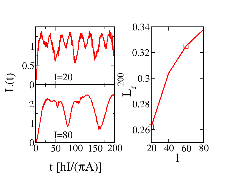
Figure 6: Left panels: Negativity $L(t)$ for $I=20,80$ and $M_{r}=0.8$, $J_{ex}/(A/2I)=3.5$, $\Delta=0$. Right panel: Maximal relative negativity $L_{r}^{200}$ in the time interval $[0,200](hI/\pi A)$ as a function of spin length $I$ for otherwise identical parameters. We find a clearly increasing curve, indicating that for large enough sizes, the baths can be fully entangled.

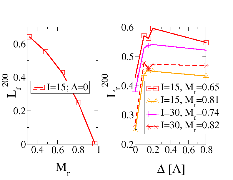
Figure 7: Left panel: Maximal relative negativity $L_{r}^{200}$ versus $M_{r}$ for $I=15$, $\Delta=0$ and the same initial state as in Fig. 6. Right panel: $L_{r}^{200}$ as a function of the detuning $\Delta$ for various parameters. The precise value of the detuning is again of no particular importance.

Conclusions.–In summary we have studied the spin and entanglement dynamics of the nuclear baths in a double quantum dot. Each of the two electron spins was considered to interact with an individual bath via homogeneous couplings. In order to lower the dimension of the problem, both baths have been approximated by long spins. We focused on the virtue of the hyperfine interaction and regarded the electron spins as an effective coupling between the baths. We demonstrated that it is possible to swap them if their size is large enough, and provided strong indication that, under the same conditions, it might be even possible to fully entangle them. Surprisingly, it turns out to be advantageous to use dots of different geometry (enabling for $\Delta\neq 0$) to built up the double quantum dot.

Acknowledgments.–This work was supported by DFG via SFB 631.

References

- (1) D. Loss and D. P. DiVincenzo, Phys. Rev. A 57, 120 (1998).
- (2) R. Hanson, L. P. Kouwenhoven, J. R. Petta, S. Tarucha, and L. M. K. Vandersypen, Rev. Mod. Phys. 79, 1217 (2007).
- (3) A. V. Khaetskii and Y. V. Nazarov, Phys. Rev. B 61, 12639 (2000).
- (4) A. V. Khaetskii and Y. V. Nazarov, Phys. Rev. B 64, 125316 (2001).
- (5) V. N. Golovach, A. V. Khaetskii, and D. Loss, Phys. Rev. Lett. 93, 016601 (2004).
- (6) A. V. Khaetskii, D. Loss, and L. Glazman, Phys. Rev. Lett. 88, 186802 (2002).
- (7) A. V. Khaetskii, D. Loss, and L. Glazman, Phys. Rev. B 67, 195329 (2003).
- (8) J. R. Petta, A. C. Johnson, J. M. Taylor, E. A. Laird, A. Yacoby, M. D. Lukin, C. M. Marcus, M. P. Hanson, and A. C. Gossard, Science 309, 2180 (2005).
- (9) F. H. L. Koppens, C. Buizert, K. J. Tielrooij, I. T. Vink, K. C. Nowack, T. Meunier, L. P. Kouwenhoven, and L. M. K. Vandersypen, Nature 442, 766 (2006).
- (10) P. F. Braun, X. Marie, L. Lombez, B. Urbaszek, T. Amand, P. Renucci, V. K. Kalevick, K. V. Kavokin, O. Krebs, P. Voisin, and Y. Masumoto, Phys. Rev. Lett. 94, 116601 (2005).
- (11) J. Schliemann, A. V. Khaetskii, and D. Loss , J. Phys.: Condens. Mat. 15, R1809 (2003).
- (12) W. Zhang, N. Konstantinidis, K. A. Al-Hassanieh, and V. V. Dobrovitski, J. Phys.: Condens. Mat. 19, 083202 (2007).
- (13) D. Klauser, W. A. Coish, and D. Loss, Chapter 10 in Semiconductor Quantum Bits, eds. O. Benson and F. Henneberger, (World Scientific, 2008).
- (14) W. A. Coish and J. Baugh, phys. stat. sol. B 246, 2203 (2009).
- (15) J. M. Taylor, J. R. Petta, A. C. Johnson, A. Yacoby, C. M. Marcus, and M. D. Lukin, Phys. Rev. B 76, 035315 (2007).
- (16) H. O. H. Churchill, A. J. Bestwick, J. W. Harlow, F. Kuemmeth, D. Marcos, C. H. Stwertka, S. K. Watson, and C. M. Marcus, Nature 5, 321 (2009).
- (17) E. Abe, K. M. Itoh, J. Isoya, and S. Yamasaki, Phys. Rev. B 70, 033204 (2004).
- (18) F. Jelezko, T. Gaebel, I. Popa, A. Gruber, and J. Wrachtrup, Phys. Rev. Lett. 92, 076401 (2004).
- (19) L. Childress, M. V. G. Dutt, J. M. Taylor, A. S. Zibrov, F. Jelezko, J. Wrachtrup, P. R. Hemmer, and M. D. Lukin, Science 314, 281 (2006).
- (20) R. Hanson, V. V. Dobrovitski, A. E. Feiguin, O. Gywat, and D. D. Awschalom , Science 320, 352 (2008).
- (21) H. Schwager, J. I. Cirac, and G. Giedke, Phys. Rev. B 81, 045309 (2010).
- (22) H. Schwager, J. I. Cirac, and G. Giedke, New J. Phys. 12, 043026 (2010).
- (23) J. M. Taylor, A. Imamoglu, and M. D. Lukin, Phys. Rev. Lett. 91, 246802 (2003).
- (24) H. Christ, J. I. Cirac, and G. Giedke, Solid State Sciences 11, 965-969 (2009).
- (25) H. Christ, J. I. Cirac, and G. Giedke, Phys. Rev. B 75, 155324 (2007).
- (26) J. M. Taylor, C. M. Marcus, and M. D. Lukin, Phys. Rev. Lett. 90, 206803 (2003).
- (27) J. J. L. Morton, A. M. Tyryshkin, R. M. Brown, S. Shankar, B. W. Lovett, A. Ardavan, T. Schenkel, E. E. Haller, J. W. Ager, and S. A. Lyon, Nature 455, 1085 (2008).
- (28) G. Austing, C. Payette, G. Yu, and J. Gupta, Jpn. J. Appl. Phys. 48, 04C143 (2009).
- (29) H. Christ, J. I. Cirac, and G. Giedke, Phys. Rev. B 78, 125314 (2008).
- (30) W. A. Coish and D. Loss, Phys. Rev. B 70, 195340 (2004).
- (31) W. A. Coish and D. Loss, Phys. Rev. B 72, 125337 (2005).
- (32) D. Klauser, W. A. Coish, and D. Loss, Phys. Rev. B 73, 205302 (2006).
- (33) D. Klauser, W. A. Coish, and D. Loss, Phys. Rev. B 78, 205301 (2008).
- (34) B. Erbe and J. Schliemann, Phys. Rev. B 81, 235324 (2010)
- (35) J. Schliemann, A. V. Khaetskii, and D. Loss, Phys. Rev. B 66, 245303 (2002).
- (36) B. Erbe and J. Schliemann, J. Phys. A: Math. Theor. 43, 492002 (2010)
- (37) M. Bortz and J. Stolze, J. Stat. Mech. P06018 (2007).
- (38) B. Erbe and H.-J. Schmidt, J. Phys. A: Math. Theor. 43, 085215 (2010).
- (39) C. Deng and X. Hu, Nanotechnology 4, 35 (2005).
- (40) W. K. Wootters, Phys. Rev. Lett. 80, 2245 (1998).
- (41) G. Vidal and R. F. Werner, Phys. Rev. A 65, 032314 (2002).
- (42) M. Plenio, Phys. Rev. Lett. 95, 090503 (2005).
- (43) A. Peres, Phys. Rev. Lett. 77, 1413 (1996).
- (44) P. Maletinsky, Ph.D. thesis, ETH Zuerich (2008).
- (45) J. Baugh, Y. Kitamura, K. Ono, and S. Tarucha, Phys. Rev. Lett. 99, 096804 (2007).
- (46) J. Baugh, Y. Kitamura, K. Ono, and S. Tarucha, phys. stat. sol. (c) 5, 302 (2008).
- (47) R. Takahashi, K. Kono, S. Tarucha, and K. Ono, arXiv:1012.4545 (2010).
- (48) A. Datta, S. Flammia, and C. Caves, Phys. Rev. A 72, 042316 (2005).