Kolmogorov and Bolgiano scaling in thermal convection:
the case of Rayleigh-Taylor turbulence

Abstract

We investigate the statistical properties of Rayleigh-Taylor turbulence in a convective cell of high aspect ratio, in which one transverse side is much smaller that the others. We show that the scale of confinement determines the Bolgiano scale of the system, which in the late stage of the evolution is characterized by the Kolmogorov-Obukhov and the Bolgiano-Obukhov phenomenology at small and large scales, respectively. The coexistence of these regimes is associated to a three to two-dimensional transition of the system which occurs when the width of the turbulent mixing layer becomes larger that the scale of confinement.

Turbulent thermal convection appears in many natural phenomena, from heat transport in stars to turbulent mixing in the atmosphere and the oceans, and in technological applications Siggia (1994); Ahlers et al. (2009); Niemela et al. (2000). Turbulent convection is driven by buoyancy forces generated by temperature fluctuations. These are then mixed by the turbulent flow itself up to small scales at which molecular diffusivity becomes important. A fundamental problem in thermal convection is the determination of the statistical properties of velocity and temperature fluctuations in the inertial range of scales in which turbulent mixing is at work.

A first step in this direction was done by Obukhov Obukhov (1949) and Corrsin Corrsin (1951) who generalized the Kolmogorov argument for the statistics of a temperature field in the so-called passive limit, in which the effects of the buoyancy forces on the velocity field are neglected Shraiman and Siggia (1990). An alternative prediction was proposed by Bolgiano Bolgiano Jr (1959) and Obukhov Obukhov (1959), in discussing the statistics of velocity and temperature fluctuations in a stably stratified atmosphere. The buoyancy forces allow to introduce in the inertial range a characteristic scale, the Bolgiano scale $L_{B}$, above which the statistics of the velocity and temperature is determined by the balance between the buoyancy and inertia forces. In spite of many years of experimental and numerical investigations, no clear evidence of this scenario has been given Lohse and Xia (2010).

In this Letter we show that in three-dimensional Rayleigh-Taylor turbulent convection the Bolgiano scale is determined by the geometrical scales of the setup. By confining the flow in a box with one dimension (e.g. $y$) much smaller than the other two, the scale $L_{y}$ becomes the Bolgiano scale of the system. By means of state of the art numerical simulations of primitive equations we find coexistent Kolmogorov-Obukhov scaling at scales smaller than $L_{y}$ and Bolgiano scaling at scales larger than $L_{y}$. Our geometrical interpretation of the Bolgiano scale suggests a new direction for numerical and experimental investigations of scaling properties in thermal convection.

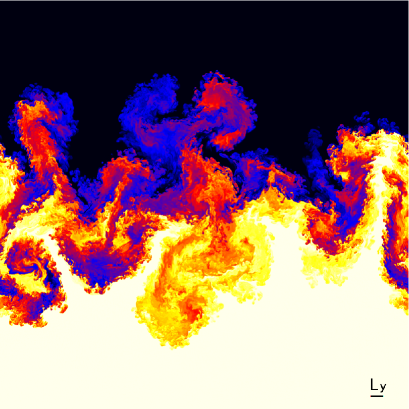
Figure 1: Central part of a vertical $(x,z)$ section of the temperature field (white=hot, black=cold) from a direct numerical simulations of Boussinesq equations (1) at resolution $4096\times 128\times 8192$ taken at time $t=3.0\tau$ (see text for the definition of $\tau$). Parameters are $\beta g=0.5$, $\nu=\kappa=2\times 10^{-5}$ and the initial temperature jump is $\theta_{0}=1$. The picture clearly shows that large-scale 2D structures coexist with small-scale 3D turbulence. The segment represents the transverse size $L_{y}$.

Rayleigh-Taylor (RT) turbulence is one of the simplest configurations of thermal convection in which a cold, heavier layer of fluid is placed on the top of an hot, lighter layer in a gravitational field. Rayleigh-Taylor instability occurs in several phenomena ranging from geophysics, to astrophysics to technological applications Schultz and et al. (2006); Cabot and Cook (2006); Isobe et al. (2005). The gravitational instability develops in an intermediate layer of turbulent fluid (the mixing layer) the width of which grows in time.

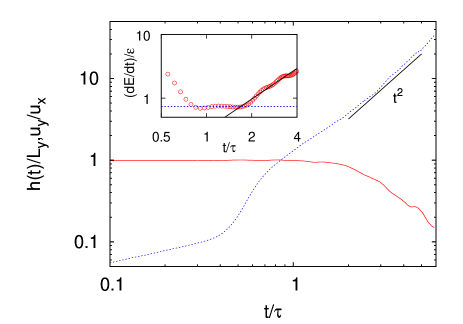
Figure 2: Temporal evolution of the mixing layer width $h(t)$ (blue, dashed line) and the ratio of $y$ component to $x$ component of rms velocity fluctuations (red, solid line). Inset: Ratio between kinetic energy growth rate $dE/dt$ and energy dissipation rate $\varepsilon$ as a function of time. The horizontal line indicates a constant ratio $\sim 0.75$ and the continuous line represents the scaling $t^{8/5}$.

We consider miscible RT turbulence at low Atwood numbers. Within the Boussinesq approximation, the equations for the dynamics of the velocity field ${\bf u}$ coupled to the temperature field $T({\bf x},t)$ (which is proportional to the density $\rho$ via the thermal expansion coefficient $\beta$ as $\rho=\rho_{0}[1-\beta(T-T_{0})]$ where $\rho_{0}$ and $T_{0}$ are reference values) read:

$$\partial_{t}{\bf u}+{\bf u}\cdot{\bf\nabla}{\bf u} = -(1/\rho_{0}){\bf\nabla}p+\nu\nabla^{2}{\bf u}-\beta{\bf g}T$$

$$\partial_{t}T+{\bf u}\cdot{\bf\nabla}T = \kappa\nabla^{2}T$$ (1)

together with the incompressibility condition ${\bf\nabla}\cdot{\bf u}=0$. In (1) ${\bf g}=(0,0,-g)$ is gravity acceleration, $\nu$ is the kinematic viscosity and $\kappa$ is the thermal diffusivity. The initial condition for the RT problem is an unstable temperature jump $T({\bf x},0)=-(\theta_{0}/2)sgn(z)$ in a fluid at rest ${\bf u}({\bf x},0)=0$.

As the system evolves, the available potential energy $P=-\beta g\langle zT\rangle$ is converted into kinetic energy $E=(1/2)\langle|{\bf u}|^{2}\rangle$ at a rate that can be estimated from the energy balance:

$$-{dP\over dt}=\beta g\langle wT\rangle={dE\over dt}+\varepsilon$$ (2)

where $w$ is the vertical velocity and $\varepsilon=\nu\langle(\partial_{\alpha}u_{\beta})^{2}\rangle$ is the viscous energy dissipation rate. From the dimensional balance between the loss of potential energy and the increase of kinetic energy one has that typical velocity fluctuations grow as $u_{rms}\simeq\beta g\theta_{0}t$, and therefore the width of the turbulent mixing layer $h(t)$, shown in Fig. 2, grows following the accelerated law $h(t)\simeq\beta g\theta_{0}t^{2}$. The integral scale $L(t)$ of the turbulent flow, defined as the largest scale on which kinetic energy is injected, is expected to grow proportionally to the geometrical scale $h(t)$ Boffetta et al. (2010).

According to the phenomenological theory of RT turbulence, developed in Chertkov (2003), the scaling behavior of the velocity and temperature fluctuations in the range of scales between the integral scale $L$ and the dissipative scale $\eta$ strongly depends on the dimensionality of the flow.

For the three-dimensional (3D) case, one assumes that the buoyancy force $\beta{\bf g}T$ balances the inertia term in (1) at the integral scale $L(t)$ and becomes negligible as the cascade proceeds towards small scales, consistently with the Kolmogorov–Obukhov phenomenology. For velocity and temperature fluctuations $\delta u(r)=u(x+r)-u(x)$ ($u$ denoting one velocity component) and $\delta T(r)=T(x+r)-T(x)$ one therefore expects Chertkov (2003)

$$\begin{array}[]{l}\delta u(r)\simeq\varepsilon^{1/3}r^{1/3}\\ \delta T(r)\simeq\varepsilon_{T}^{1/2}\varepsilon^{-1/6}r^{1/3}\end{array}$$ (3)

where the energy dissipation rates $\varepsilon$ grows in time as $\varepsilon(t)\simeq(\beta g\theta_{0})^{2}t$, following adiabatically the dynamics of the large eddies, while the temperature dissipation rates decreases as $\varepsilon_{T}(t)\simeq\theta_{0}^{2}t^{-1}$ Cabot and Cook (2006); Boffetta et al. (2009).

This scenario is not consistent in two dimensions (2D) where kinetic energy is transferred toward large scales developing an inverse cascade Kraichnan and Montgomery (1980). In this case the buoyancy term injects energy at all scales generating a non-constant-in-wavenumber energy flux. As a consequence, velocity and temperature fluctuations follow the Bolgiano-Obukhov scaling Chertkov (2003)

$$\begin{array}[]{l}\delta u(r)\simeq\varepsilon_{T}^{1/5}(\beta g)^{2/5}r^{3/5}\\ \delta T(r)\simeq\varepsilon_{T}^{2/5}(\beta g)^{-1/5}r^{1/5}\end{array}$$ (4)

which has been verified in numerical simulations of 2D RT turbulence Celani et al. (2006).

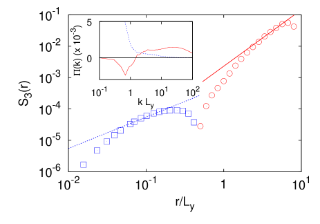
Figure 3: Third order longitudinal velocity structure function $S_{3}(r)$ (red circles) and $-S_{3}(r)$ (blue squares) computed in the mixing layer. The two lines represent Kolmogorov scaling $r$ (blue dotted) and Bolgiano scaling $r^{9/5}$ (red continuous). Inset: contribution to the energy flux in Fourier space $\Pi(k)$ from the nonlinear term (red, continuous line) and from the buoyancy term (blue, dashed line).

Let us consider now a convective cell with large aspect ratio $L_{x},L_{z}\gg L_{y}$. At short times, when $L(t)<L_{y}$ the turbulent flow in the mixing layer can be considered three-dimensional and a direct cascade with Kolmogorov-Obukhov scaling (3) is expected. At later times, when $L(t)>L_{y}$ the flow cannot be fully three dimensional at large scales, as a consequence of the geometrical constrain in the $y$ direction. The question arises whether the two-dimensional phenomenology appears at scales $L_{y}<r<L(t)$. For this to happen most of the injected by buoyancy forces should go to large scales producing an inverse cascade with Bolgiano-Obukhov scaling (4). However, a residual direct cascade to scales $r<L_{y}$ should be present with a flux $\varepsilon(t)$ given by the matching of the scaling (3) and (4) at $r=L_{y}$:

$$\varepsilon(t)\simeq(\beta g\theta_{0})^{6/5}L_{y}^{4/5}t^{-3/5}$$ (5)

The time of the transition from 3D to 2D behavior is given by continuity requirement in energy dissipation, i.e. equating (5) with 3D dissipation $(\beta g\theta_{0})^{2}t$ which gives $\tau=(L_{y}/(\alpha\beta g\theta_{0}))^{1/2}$ where $\alpha\simeq 0.02$ is a dimensionless number obtained from numerical simulations Boffetta et al. (2009).

Summarizing, the long-time behavior of RT turbulence with large aspect ratio is the following. A small scales $\eta\leq r\leq L_{y}$ a three-dimensional direct cascade with Kolmogorov-Obukhov scaling is expected. At large scales $L_{y}\leq r\leq L(t)\sim t^{2}$ a two-dimensional inverse cascade with Bolgiano-Obukhov scaling should be observed.

The above predictions have been tested against the results of state of the art, high resolution numerical simulations of equations (1), is a large aspect ratio geometry with $L_{z}/L_{x}=2$, $L_{y}/L_{x}=1/32$, in which the flow thus results strongly confined in the $y$ direction. The integration of equations (1), discretized on a $4096\times 128\times 8192$ grid with periodic boundary conditions, has been performed with a fully parallel pseudospectral code, with $2/3$-dealiasing, running on a IBM-SP6 supercomputer.

Figure 1 shows a vertical section of the temperature field in the late stage of the simulations. Large scales, 2D structures are clearly observed.

As shown in Figure 2, at $t\simeq\tau$, when the mixing layer scale $h(t)$ becomes of the order of $L_{y}$ the flow becomes increasingly anisotropic with $u_{y}\ll u_{x},u_{z}$. In this conditions, we observe a transition from 3D to 2D turbulent behavior, clearly signaled by a change in the ratio between the energy growth rate $dE/dt$ and the viscous dissipation rate $\varepsilon$ (the energy flux to small scales in the direct cascade). In the 3D regime both these quantities grow linearly in time and therefore their ratio is constant. After the transition the inverse cascade sets in and $(dE/dt)/\varepsilon\sim t^{8/5}$, as follows from (2) and (5). Both behaviors are evident in Fig. 2.

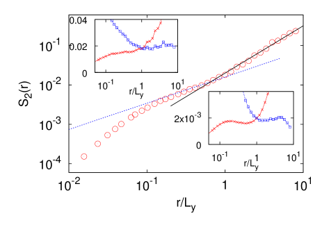
Figure 4: Second-order longitudinal velocity structure function $S_{2}(r)$. The two lines represent Kolmogorov scaling $r^{2/3}$ (blue dotted) and Bolgiano scaling $r^{6/5}$ (red continuous). Upper inset: Second-order structure function $S_{2}(r)$ compensated with Kolmogorov (red crosses) and Bolgiano (blue squares) scaling. Lower inset: Fourth-order structure function $S_{4}(r)$ compensated with Kolmogorov (red crosses) and Bolgiano (blue squares) scaling.

In the late stage of the evolution, when $L(t)>L_{y}$ we expect the simultaneous presence of a direct and an inverse cascade in the two range of scales $r<L_{y}$ and $r>L_{y}$, respectively. This can be verified by computing the scale dependent energy flux, given by the third-order structure function of longitudinal velocity increments (i.e. taken along the local velocity direction) $S_{3}(r)\equiv\langle(\delta_{\parallel}u(r))^{3}\rangle$. For isotropic three dimensional turbulence, the classical result due to Kolmogorov predicts Frisch (1995) $S_{3}(r)=-(4/5)\varepsilon r$.

As shown in Fig. 3, at small scales $r<L_{y}$ $S_{3}(r)$ is negative and, in a narrow range of scales, compatible with the Kolmogorov prediction $S_{3}(r)\sim r$. At scales $r>L_{y}$, $S_{3}(r)$ becomes positive, signaling the reversal of the energy cascade, and displays a scaling behavior $S_{3}(r)\sim r^{9/5}$ consistent with (4).

The inset of Fig. 3 shows the contributions of the inertia and buoyancy terms to the energy flux in Fourier space $\Pi(k)\equiv(d/dt)\int_{k}^{\infty}E(p)dp$ where $E(p)$ is the energy spectrum and time derivative is computed by taking into account, separately, the non-linear and buoyancy terms of (1). Al low wavenumbers $kL_{y}<1$ the buoyancy contribution is dominant, and the negative sign of the inertial contribution to the energy flux confirms the presence of a 2D inverse cascade. At high wavenumbers $kL_{y}>1$ the buoyancy contribution becomes sub-dominant, and one recovers a constant positive flux characteristic of the 3D regime Frisch (1995).

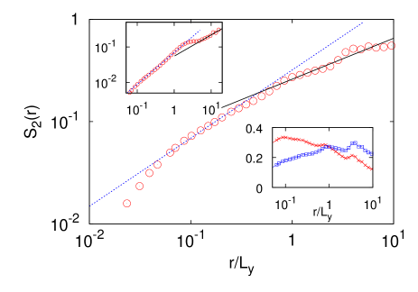
Figure 5: Second-order temperature structure function $S_{2}(r)$. The two lines represent Kolmogorov scaling $r^{2/3}$ (blue dotted) and Bolgiano scaling $r^{2/5}$ (red continuous). Lower inset: Second-order structure function $S_{2}(r)$ compensated by Kolmogorov (red crosses) and Bolgiano (blue squares) scaling. Upper inset: Fourth-order temperature structure function together with power laws corresponding to best fit scaling at small scales $r^{0.9}$ (blue dotted) and at large scales $r^{0.6}$ (red continuous).

The coexistence of Kolmogorov-Obukhov scaling at small scales and Bolgiano-Obukhov scaling at large scales is confirmed by behavior of the structure functions of longitudinal velocity increments $S_{p}(r)\equiv\langle(\delta_{\parallel}u(r))^{p}\rangle$ and of temperature increments $S^{T}_{p}(r)\equiv\langle(\delta T(r))^{p}\rangle$, shown in Figures 4 and 5. The transition between the two regimes occurs at the Bolgiano scale which is found to be $r\simeq L_{y}$.

In three dimensional turbulence, small deviations from the dimensional predictions are expected in the scaling of the velocity fluctuations, indicating the presence of small scale intermittency Frisch (1995). Here, we found much stronger corrections in the statistics of temperature fluctuations, whose $4$-th order structure function strongly differs from the dimensional scaling at small scales with a best fit exponent $0.9$ close to the corresponding exponent for passive scalar in three-dimensional turbulence. At large scale, temperature structure functions show strong fluctuations due to the presence of regions of unmixed fluid within the mixing layer, as shown in Fig. 1. Nonetheless, a very short range of scaling also for the $4$-th order structure function is observed with a scaling exponent close to the intermittent value $0.6<4/5$ measured in pure $2D$ RT simulations Celani et al. (2006).

Our numerical findings supports the phenomenological prediction that in RT convection the Bolgiano scale is determined by the aspect ratio of the convective cell. The presence of Bolgiano-Obukhov scaling is associated to a dimensional transition of the flow which occurs when the width of the mixing layer becomes larger than the confining scale $L_{y}$ Celani et al. (2010); Shats et al. (2010). This poses the intriguing question on whether in generic convective systems the Bolgiano-Obukhov phenomenology could be observed whenever the turbulent flow is confined by geometrical constraints and/or physical mechanisms (such as rotation or stratification) in convective cells with small aspect ratio. Indeed, recent experiments in soap film convection observe Bolgiano scaling for large values of the Rayleigh number Zhang and Wu (2005); Seychelles et al. (2010). Despite the similarities with our results, we remark the presence of important differences, as the experimental data show both the presence of intermittency in the velocity field Zhang and Wu (2005) and the absence of intermittency in the temperature field Seychelles et al. (2010). On the contrary, our simulations shows the absence of intermittency for the velocity field which performs an inverse cascade and are compatible with some intermittency for the temperature field in the direct cascade. It would be therefore extremely interesting to have a direct comparison of experimental and numerical data on thermal convection in quasi-two-dimensional flow which would give new insights on the fundamental issue of intermittency in turbulent convection.

Numerical simulations have been done at the Cineca under the HPC-EUROPA2 project (project number: 228398) with the support of the European Commission - Capacities Area - Research Infrastructures. We thank G. Erbacci and the staff at Cineca Supercomputing Center (Bologna, Italy) for their support.

References

- Siggia (1994) E. Siggia, Ann. Rev. Fluid Mech. 26, 137 (1994).
- Ahlers et al. (2009) G. Ahlers, S. Grossmann, and D. Lohse, Rev. Mod. Phys. 81, 503 (2009).
- Niemela et al. (2000) J. Niemela, L. Skrbek, K. Sreenivasan, and R. Donnelly, Nature 404, 837 (2000).
- Obukhov (1949) A. Obukhov, Izv. Aka. Nauk. SSSR, Ser. Geograf. Geofiz 13, 58 (1949).
- Corrsin (1951) S. Corrsin, Journal of Applied Physics 22, 469 (1951).
- Shraiman and Siggia (1990) B. Shraiman and E. Siggia, Physical Review A 42, 3650 (1990), ISSN 1094-1622.
- Bolgiano Jr (1959) R. Bolgiano Jr, Journal of Geophysical Research 64, 2226 (1959).
- Obukhov (1959) A. Obukhov, in Dokl. Akad. Nauk SSSR (1959), vol. 125, p. 1246.
- Lohse and Xia (2010) D. Lohse and K. Xia, Annual Review of Fluid Mechanics 42, 335 (2010), ISSN 0066-4189.
- Schultz and et al. (2006) D. Schultz and et al., J. Atmos. Sci. 63, 2409 (2006).
- Cabot and Cook (2006) W. Cabot and A. Cook, Nature Physics 2, 562 (2006).
- Isobe et al. (2005) H. Isobe, T. Miyagoshi, K. Shibata, and T. Yokoyama, Nature 434, 478 (2005).
- Boffetta et al. (2010) G. Boffetta, A. Mazzino, S. Musacchio, and L. Vozella, Physics of Fluids 22, 035109 (2010).
- Chertkov (2003) M. Chertkov, Phys. Rev. Lett. 91, 115001 (2003).
- Boffetta et al. (2009) G. Boffetta, A. Mazzino, S. Musacchio, and L. Vozella, Phys. Rev. E 79, 065301(R) (2009).
- Kraichnan and Montgomery (1980) R. H. Kraichnan and D. Montgomery, Reports on Progress in Physics 43, 547 (1980).
- Celani et al. (2006) A. Celani, A. Mazzino, and L. Vozella, Phys. Rev. Lett. 96, 134504 (2006).
- Frisch (1995) U. Frisch, Turbulence: The Legacy of AN Kolmogorov (Cambridge University Press, 1995).
- Celani et al. (2010) A. Celani, S. Musacchio, and D. Vincenzi, Physical Review Letters 104, 184506 (2010).
- Shats et al. (2010) M. Shats, D. Byrne, and H. Xia, Phys. Rev. Lett. 105, 264501 (2010).
- Zhang and Wu (2005) J. Zhang and X. L. Wu, Phys. Rev. Lett. 94, 234501 (2005).
- Seychelles et al. (2010) F. Seychelles, F. Ingremeau, C. Pradere, and H. Kellay, Phys. Rev. Lett. 105, 264502 (2010).