NSF-KITP-11-092
Dynamical aspects of inextensible chains

Abstract

In the present work the dynamics of a continuous inextensible chain is studied. The chain is regarded as a system of small particles subjected to constraints on their reciprocal distances. It is proposed a treatment of systems of this kind based on a set Langevin equations in which the noise is characterized by a non-gaussian probability distribution. The method is explained in the case of a freely hinged chain. In particular, the generating functional of the correlation functions of the relevant degrees of freedom which describe the conformations of this chain is derived. It is shown that in the continuous limit this generating functional coincides with a model of an inextensible chain previously discussed by one of the authors of this work. Next, the approach developed here is applied to a inextensible chain, called the freely jointed bar chain, in which the basic units are small extended objects. The generating functional of the freely jointed bar chain is constructed. It is shown that it differs profoundly from that of the freely hinged chain. Despite the differences, it is verified that in the continuous limit both generating functionals coincide as it is expected.

1 Introduction

There are several physical situations in which it is required that a polymer chain is inextensible. This happens for instance when the chain is pulled at its ends by strong forces [1, 2, 3, 4, 5] in experiments of DNA micromanipulations. In order to impose the constraints in the stochastic equations governing the motion of the chain it is possible to apply a variety of powerful techniques [6, 7, 8, 9, 10, 11, 12, 13]. Progresses in the understanding of statistic and dynamical aspects of inextensible chains have been obtained mainly with the help of numerical simulations, see for example Refs. [14, 15, 16, 17, 18, 19, 20, 21]. For analytical calculations, models in which the condition of inextensibility is relaxed are usually preferred. This is the case of the gaussian chain [22], which often replaces the freely jointed chain [23] in the study of the statistical behavior of polymers systems. Other examples of theories in which the length of the chain is allowed to become infinitely long are the models of Rouse [24] and Zimm [25]. They provide a satisfactory description of the dynamics of polymer chains in solutions, but could fail in the case of a chain that is stretched under strong external forces applied at its ends.

For these reasons it is highly desirable to construct a path integral model describing the dynamics of an inextensible chain which is simple enough to allow analytic calculations. In particular, we are interested in the derivation of the generating functional of the correlation functions of the relevant variables that describe the conformation of the chain. The usual starting point is a discrete mechanical model which provides a coarse grained approximation of the chain. Successively, a continuous limit is performed, in which the number of elements becomes infinitely large and their length approaches zero, while the total length of the chain $L$ is kept constant. This limit is useful in order to smooth out the dependence on the details of the particular mechanical model chosen. In the first part of this article the case of a freely hinged chain (FHC) is considered. This is a system of beads connected together by massless links of fixed length $a$. The FHC has been studied in the past in Refs. [26, 27, 28] in connection with the dynamics of cold polymers or a gas of hot polymers. In Ref. [29] it has been shown that the generating functional for a FHC coincides in the continuous limit with the partition function of a theory which closely resembles a nonlinear sigma model. For this reason it has been called the generalized nonlinear sigma model or simply GNL$\sigma$M. Within the GNL$\sigma$M it is possible to perform analytical calculations of physical quantities that can be applied to study the dynamics of cold chains or of chains moving in a very viscous environment [29, 30, 31]. One drawback of the GNL$\sigma$M is that it regards the FHC as a gas of fluctuating particles with the inextensibility constraints being implemented by means of a product of delta functions. The introduction of delta functions to fix constraints is a standard procedure in the investigations of the statistical mechanics of polymers, where it is an useful tool in order to limit the conformations of the chain. In the case of dynamics, however, a physical explanation of the appearance of the delta functions inside the path integral of the GNL$\sigma$M is necessary, otherwise the connection with the stochastic process of the fluctuating chain is lost. Such connection was up to now somewhat obscure, despite the fact that in Ref. [32] it has been possible to verify that the GNL$\sigma$M reproduces as expected the sum over all chain conformations satisfying a free Langevin equation and subjected to constraints that ensure the property of inextensibility.

One goal of this work is to provide a physical interpretation of the GNL$\sigma$M as a stochastic process in which the noise is non-gaussian. The starting point is the observation that the chain degrees of freedom which are constrained by the inextensibility requirement are frozen and thus cannot be influenced by the noise. This implies that the noise must be constrained too. The conditions on the noise are imposed in the present approach in a soft way using an elastic potential. It is the introduction of this potential that modifies the noise distribution and makes it non-gaussian. The rigid constraints are recovered in the limit in which the elastic constants become infinite. Following this strategy, the motion of the beads of the chain is described by a system of free Langevin equations in which the random forces are characterized by a non-gaussian distribution. For any finite value of the elastic constants, the related generating functional corresponds to that of a chain consisting of beads connected together by springs. With increasing values of the elastic constants, the springs become stiffer and stiffer until at the end an inextensible chain is obtained. Let us note that also the beads of the Rouse model are joined together by springs. However, in that model the potentials are chosen in such a way that the springs are in their rest positions only when the distances between neighboring beads is zero. For this reason, in the limit of infinite elastic constants, the chain collapses to a point. Other differences of the GNL$\sigma$M from the Rouse model have been discussed in details in Ref. [29]. The present strategy to enforce the inextensibility constraints with the help of potentials closely resembles the way in which stiff constraints (sometimes called flexible constraints) are imposed [20, 21] in stochastic equations. Stiff constraints are fixed in fact with the help of potentials [33, 34] whose role is to create an energy barrier that strongly suppresses those chain conformations that do not satisfy the constraints. The form of these potentials, like for instance the FENE potential, is usually too complicated to allow analytic calculations. In the case of the GNL$\sigma$M, instead, there are only elastic potentials, which are relatively simple. Another striking difference with respect to stiff constraints is that in our approach it is taken the limit in which the strength of the elastic forces become infinite. In this limit the constraints become rigid and not flexible.

In the second part of this work the idea of Ref. [5] is investigated. According to that idea, a chain may be realized by connecting together basic inextensible units, like for instance small bars. In this way, the length of all elements of the resulting chain is always constant by construction without the need of imposing the cumbersome holonomic constraints that are otherwise necessary to enforce the property of inextensibility. Constraints are still necessary in order to connect together the basic units, but they are very simple and their imposition is straightforward. In deriving the generating functional for a system of this kind, however, the fact that the basic inextensible units are not point-like objects, but rigid bodies with rotational degrees of freedom, is the origin of several complications. For this reason, in this work the basic inextensible units are built starting from a number $K$ of beads of diameter $\Delta l$, called hereafter spheres. The motion of the spheres is constrained in such a way that they stay aligned along a segment of fixed length. The shape of the whole system formed by the $K$ spheres is that of a shish-kebab and offers a good approximation of a bar. Let us note that the constraints needed in order to form the shish-kebabs consist in conditions on the distances between pairs of points. Thus we can apply the same strategy used to implement the inextensibility constraints in the FHC, which are of the same type. In the limit in which the number of spheres approaches infinity and their radius becomes vanishingly small, while the length of the basic units remains constant, one obtains what has been called here the freely jointed bar chain or simply FJBC. This is a discrete chain composed by one-dimensional bars with uniform distribution of mass.

The expression of the generating functional of the correlation functions of the shish-kebab chain has been provided in the most general case of a chain containing $N$ basic units, each composed by a number $K$ of beads. The generating functional of the FJBC in the limit $K\to+infty$ and $\Delta l\to 0$ has been derived. As discussed in [5], the constraints that are needed to held together the basic units are almost trivial and the associated spurious degrees of freedom can be easily eliminated. Finally, the continuous limit of the generating functional of the FJBC has been performed. In this case several simplifications occur and, at the end, it has been possible to prove that the generating functional of the resulting continuous system coincides with the GNL$\sigma$M. This is an expected result, because in the continuous limit the mechanical details of the underlying discrete chain should not play any role.

The material presented in this paper is organized as follows. In Section 2 the classical aspects of the FHC and the FJBC are analyzed. For the interested reader, a more extensive discussion on this subject can be found in Ref. [35]. First, the case of the FHC is briefly reviewed. Next, the FJBC is studied. It is shown that, while the kinetic and potential energies of the FJBC differ considerably from those of the FHC, they coincide in the continuous limit. The discussion of the classical aspects of the chain dynamics is very important to establish a mathematically convenient description of the FJBC, that will be used later to study its statistical dynamics. The classical dynamics of inextensible chains is also very interesting for concrete applications ranging from cosmetics to computer graphics. Section 3 is dedicated to the statistical dynamics of the chain. In the first part of that Section, the generating functional of the correlation functions of the radius vectors which specify the positions of the beads of the FHC is derived in path integral form. The constraints required by the fact that the length of the links connecting the beads is constant are imposed by using elastic potentials as explained before. When the strength of these potentials becomes infinite, the path integral formulation of the generating functional of the FHC given in Ref. [29] is recovered. In the continuous limit the GNL$\sigma$M is obtained. We fill also a gap of our previous publications concerning the FHC by establishing the connection of the partition function of the FHC with a stochastic process described by a Fokker–Planck equation. In the second part of Section 3 the generating functional of the FJBC in the shish-kebab approximation is derived. Next, in Section 4 we compute the generating functional of the FJBC without any approximation. In analogy with what happens in the classical case, it turns out that this generating functional is very different from that of the FHC. However, we are able to show that they both coincide in the limit of a continuous chain. Finally, our conclusions are drawn in Section 5.

2 Classical dynamics

2.1 The freely hinged chain (FHC)

We begin by studying the dynamics of a chain composed by $N$ beads of mass $m$ joined together by $N-1$ massless segments of length $a$. Though it is not strictly necessary, to avoid complications with the spherical coordinates in arbitrary dimensions, in this Section the discussion will be limited to two dimensional chains moving on the $(x,y)$ plane. Let $\bm{R}_{i}(t)=(x_{i}(t),y_{i}(t))$ denote the radius vector of the $i-$th bead, for $i=1,\ldots,N$. In polar coordinates (see Fig. 1):

$$x_{i}(t) = \sum_{j=1}^{i-1}a\sin\alpha_{j}(t)\qquad\qquad i=2,\ldots,N$$ (1)

$$y_{i}(t) = \sum_{j=1}^{i-1}a\cos\alpha_{j}(t)\qquad\qquad i=2,\ldots,N$$ (2)

We suppose that the first point $(i=1)$ is fixed in the origin, so that:

$$x_{1}(t)=y_{1}(t)=0$$ (3)

Figure 1: FHC consisting of $N$ beads of mass $m$ (the black circles) connected together by $N-1$ segments of fixed length $a$. The angles between the $y$ axis and the $i-$th segment are denoted by $\alpha_{i}$, $i=1,\ldots,N-1$.

First of all, we compute the kinetic energy of the system:

$$T_{FHC}(a)=\sum_{i=2}^{N}\frac{m}{2}\left(\dot{x}^{2}_{i}(t)+\dot{y}^{2}_{i}(t)\right)$$ (4)

The dots denote here derivatives with respect to the time $t$, i. e. $\dot{x}=\frac{\partial x}{\partial t}$. After a few calculations we find the expression of $T_{FHC}(a)$ in polar coordinates:

$$T_{FHC}(a)=\frac{ma^{2}}{2}\sum_{i=2}^{N}\sum_{j,k=1}^{i-1}\dot{\alpha}_{j}\dot{\alpha}_{k}\cos(\alpha_{j}-\alpha_{k})$$ (5)

We are interested in the continuous chain obtained from the FHC after performing the limit in which the length $a$ of the segments goes to zero while the total length $L$ of the chain is preserved:

$$a\longrightarrow 0\qquad N\longrightarrow+\infty\qquad\mbox{and}\qquad Na=L$$ (6)

In that limit the sums become integrals according to the prescription:

$$\sum_{i=2}^{N}a\to\int_{0}^{L}ds\qquad\qquad\sum_{j=1}^{i-1}a\to\int_{0}^{s}du$$ (7)

A function $f_{i}(t)$ depending on the discrete index $i$, like for instance the angles $\alpha_{i}(t)$, will be substituted by a function of the continuous variable $s$, where $0\leq s\leq L$, according to the rule: $f_{i}(t)\longrightarrow f(t,s)$. The full procedure to pass to the continuous limit (6) is described in Ref. [29, 36] and will not be discussed here. The new parameter $s$ appearing in (7) is the arc–length that measures the distance between two points on the chain. Partial derivatives with respect to $s$ will be denoted with a prime, for instance $\bm{R}^{\prime}(t,s)=\frac{\partial\bm{R}(t,s)}{\partial s}$. We also need to express the mass of the beads $m$ as a function of $a$. To this purpose, we introduce the density of mass $\rho$ on the chain. Since the mass distribution is uniform – all beads have the same mass – we may put $\rho=\frac{M}{L}$, where $M$ is the total mass of the chain. Thus, $m$ can be written as a function of the mass density:

$$m=\frac{M}{L}a$$ (8)

It is easy to check that, for consistency, $Nm=M$ because $Na=L$. Applying the above prescriptions, it is possible to show that the continuous kinetic energy $T_{FHC}=\lim\limits_{a\to 0,N\to+\infty,Na=L}T_{FHC}(a)$ is given by:

$$T_{FHC}=\frac{M}{2L}\int_{0}^{L}ds\int_{0}^{s}du\int_{0}^{s}dv{\dot{\alpha}}(t,u){\dot{\alpha}}(t,v)\cos\left(\alpha(t,u)-\alpha(t,v)\right)$$ (9)

Let us note that the expression of $T_{FHC}$ given above is different from that of Ref. [29]. This is due to the fact that here we have not followed the recursive procedure for computing $T_{FHC}(a)$ used in [29], but rather we have derived it directly from the definition of kinetic energy of Eq. (4). It is possible to show the equivalence of the results obtained in this work and in Ref. [29] exploiting the identity:

$$\int_{0}^{s}du\int_{0}^{s}dvf(u,v)=\int_{0}^{s}du\int_{0}^{u}dvf(u,v)+\int_{0}^{s}du\int_{0}^{u}dvf(v,u)$$ (10)

which is valid for an arbitrary integrable function $f$ of $v$ and $u$. Exploiting Eq. (10), the kinetic energy $T_{FHC}$ in (9) becomes:

$$T_{FHC}=\frac{M}{L}\int_{0}^{L}ds\int_{0}^{s}du\int_{0}^{u}dv\dot{\alpha}(t,u)\dot{\alpha}(t,v)\cos(\alpha(t,u)-\alpha(t,v))$$ (11)

The right hand side of the above equation coincides exactly with the kinetic energy of the $FHC$ derived in [29].

Finally, we add to the FHC model the interactions. To this purpose, we define the potential:

$$V_{FHC}(a)=\sum_{i=1}^{N}aV_{E}(\bm{R}_{i}(t))+\sum_{\underset{i\neq j}{i,j=1}}^{N}a^{2}V_{I}(\bm{R}_{i}(t),\bm{R}_{j}(t))$$ (12)

where $V_{E}(\bm{R}_{i}(t))$ and $V_{I}(\bm{R}_{i}(t),\bm{R}_{j}(t))$ have the meaning of energy densities per unit of chain length due to external and internal forces respectively. For this reason, in the total potential energy of the chain $V_{FHC}(a)$ appearing in Eq. (12), $V_{E}(\bm{R}_{i}(t))$ and $V_{I}(\bm{R}_{i}(t),\bm{R}_{j}(t))$ are multiplied by the factors $a$ and $a^{2}$ respectively. The presence of these factors is in agreement with the continuous limit prescription of Eq. (7).

In the continuous limit (6) we obtain from $V_{FHC}(a)$:

$${\normalsize V_{FHC}=}\lim_{a\to 0,N\to+\infty,Na=L}V_{FHC}(a)=\int_{0}^{L}{\normalsize dsV}_{E}{\normalsize(\bm{R}(t,s))+}\int_{0}^{L}ds\int_{0}^{L}ds^{\prime}V_{I}{\normalsize(\bm{R}(t,s),\bm{R}(t,s}^{\prime}{\normalsize))}$$ (13)

where $\bm{R}(t,s)$ is the continuous limit of the bond vectors $\bm{R}_{i}(t)$. From Eqs. (1) and (2) it turns out that the components of $\bm{R}(t,s)$ are given by:

$$\bm{R}{\normalsize(t,s)=}\int_{0}^{s}{\normalsize du(}\sin{\normalsize\alpha(t,u),}\cos{\normalsize\alpha(t,u))}$$ (14)

2.2 The case of the FJBC

Let us consider a chain composed by ${\normalsize N}$ bars of length ${\normalsize a}$. Each bar is regarded here as a one-dimensional segment with a uniform distribution of mass along it. The bars are joined at the points:

$$x_{i}=\sum\limits_{i^{{}^{\prime}}=1}^{i-1}a\sin\alpha_{i^{{}^{\prime}}}.$$ (15)

$$y_{i}=\sum\limits_{i^{{}^{\prime}}=1}^{i-1}a\cos\alpha_{i^{{}^{\prime}}}.$$ (16)

where $i=2,\ldots,N$. One end of the first bar is supposed to be fixed in the origin, so that $x_{1}=y_{1}=0.$ The coordinates of every point of such a chain are given by:

$$x_{i}\left(t,l\right)=\sum\limits_{j=1}^{i-1}a\sin\alpha_{j}(t)+l\sin\alpha_{i}(t)$$ (17)

$$y_{i}\left(t,l\right)=\sum\limits_{j=1}^{i-1}a\cos\alpha_{j}(t)+l\cos\alpha_{i}(t)$$ (18)

for $i=2,\ldots,N-1$. The points of the first bar have coordinates:

$${\normalsize x}_{i}\left(t,l\right){\normalsize=l}\sin{\normalsize\alpha}_{i}(t)$$ (19)

$$y_{i}\left(t,l\right)=l\cos\alpha_{i}(t)$$ (20)

Here $l$ is a continuous parameter taking its values in the range $0\leq l\leq a$. In the future also the notation

$$\bm{R}_{i}(t,l)=(x_{i}(t,l),y_{i}(t,l)),\qquad i=1,\ldots,N-1$$ (21)

will be used. We are now ready to compute the kinetic energy of the FJBC:

$$T_{FJBC}(a)=\sum_{i=1}^{N-1}\int_{0}^{a}\frac{\mu_{i}}{2a}dl\left(\dot{x}_{i}^{2}(t,l)+\dot{y}_{i}^{2}(t,l)\right)$$ (22)

In the above equation $\mu_{i}$ is the mass of the $i-$th bar. We have assumed that the mass distribution of each bar is homogeneous. For that reason, the mass ${\normalsize dm}_{i}$ of a small element of length ${\normalsize dl}$ is:

$$dm_{i}=\frac{\mu_{i}}{a}dl$$ (23)

If all bars have the same mass, i. e. $\mu_{i}=\mu$ for $i=1,\ldots,N-1$, it is possible to put $dm_{i}=\frac{M}{L}dl$ using the fact that $\mu N=M$ and $aN=L$. After simple calculations we find out that:

$$T_{FJBC}(a)=\frac{M}{2L}\sum_{i=1}^{N-1}\int_{0}^{a}dl\left[\sum_{j,k=1}^{i-1}a^{2}\dot{\alpha}_{j}\dot{\alpha}_{k}\cos(\alpha_{j}-\alpha_{k})+l^{2}\dot{\alpha}_{i}^{2}+2al\sum_{j=1}^{i-1}\dot{\alpha}_{j}\dot{\alpha}_{i}\cos(\alpha_{j}-\alpha_{i})\right]$$ (24)

After the integration over $dl$ we obtain:

$$T_{FJBC}(a)=\frac{M}{2L}\sum_{i=1}^{N-1}a^{3}\left[\sum_{j,k=1}^{i-1}\dot{\alpha}_{j}\dot{\alpha}_{k}\cos(\alpha_{j}-\alpha_{k})+\frac{\dot{\alpha}_{i}^{2}}{3}+\sum_{j=1}^{i-1}\dot{\alpha}_{j}\dot{\alpha}_{i}\cos(\alpha_{j}-\alpha_{i})\right]$$ (25)

Let us note that, in order to derive the above expression of the kinetic energy, the computation of the moments of inertia of the bars has not been necessary. Each bar has been rather decomposed into a set of infinitesimal elements which can be regarded as points. The kinetic energy of each of these points has then been summed up to obtain the total kinetic energy of the chain given in Eq. (25). The result is the same as if we had considered the bars as the basic units of the chain and computed their kinetic energy. An approach in which the chain is regarded as a set of points and not as a system of bars is not a great advantage in the simple classical case. However, it will be of crucial importance when the statistical physics of the FJBC will be studied, because the Fokker-Planck equation for a bar is prohibitively complicated for our purposes.

We are now ready to perform the continuous limit (6) in which the length $a$ of the segments goes to zero while the total length $L$ of the chain is preserved. Putting

$$\lim_{a\to 0,N\to+\infty,Na=L}T_{FJBC}(a)=T_{FJBC}$$ (26)

the continuous kinetic energy takes the form:

$$T_{FJBC}=\frac{M}{2L}\int_{0}^{L}ds\int_{0}^{s}du\int_{0}^{s}dv\dot{\alpha}(t,u)\dot{\alpha}(t,v)\cos(\alpha(t,u)-\alpha(t,v))$$ (27)

Eq. (27) coincides exactly with the kinetic energy of the continuous FHC of Eq. (9).

Let’s now add to the $FJBC$ the interactions described by a general potential of the kind:

$${\normalsize V_{FJBC}(a)=}\sum_{i=1}^{N-1}\int_{0}^{a}{\normalsize dl\tilde{V}}_{E}{\normalsize(}\bm{R}_{i}{\normalsize(t,l))+}\sum_{\begin{subarray}{c}i,j=1\\ i\neq j\end{subarray}}^{N-1}\int_{0}^{a}{\normalsize dl}\int_{0}^{a}{\normalsize dl}^{\prime}{\normalsize\tilde{V}}_{I}{\normalsize(}\bm{R}_{i}{\normalsize(t,l),}\bm{R}_{j}{\normalsize(t,l}^{\prime}{\normalsize))}$$ (28)

Here $\tilde{V}_{E}(\bm{R}_{i})$ and $\tilde{V}_{I}(\bm{R}_{i},\bm{R}_{j})$ take into account the external and internal interactions respectively. In the case of small values of $a$, $V_{FJBC}(a)$ may be approximated as follows:

$${\normalsize V_{FJBC}(a)\sim}\sum_{i=1}^{N-1}{\normalsize a\tilde{V}}_{E}{\normalsize(}\bm{R}_{i}{\normalsize(t,a))+}\sum_{\begin{subarray}{c}i,j=1\\ i\neq j\end{subarray}}^{N-1}{\normalsize a}^{2}{\normalsize\tilde{V}}_{I}{\normalsize(}\bm{R}_{i}{\normalsize(t,a),}\bm{R}_{j}{\normalsize(t,a))}$$ (29)

with

$$\bm{R}_{i}{\normalsize(t,a)=}\sum_{j=1}^{i-1}{\normalsize a(}\sin{\normalsize\alpha}_{j}{\normalsize(t),}\cos{\normalsize\alpha}_{j}{\normalsize(t))}\qquad\qquad i=2,\ldots,N$$ (30)

and $\bm{R}_{1}(t)=0$. The above approximation of $V_{FJBC}(a)$ becomes exact in the continuous limit of Eq. (6), in which the expression of the potential becomes:

$${\normalsize V_{FJBC}=}\int_{0}^{L}{\normalsize ds\tilde{V}}_{E}{\normalsize(\bm{R}(t,s))+}\int_{0}^{L}{\normalsize ds\int_{0}^{L}ds^{\prime}\tilde{V}_{I}}{\normalsize(\bm{R}(t,s),\bm{R}(t,s}^{\prime}{\normalsize))}$$ (31)

where $\bm{R}(t,s)$ is given in Eq. (14). As we may see, the above expression of the potential coincides with that of the FHC of Eq. (13). As a consequence, in the continuous limit the FHC and FJBC are equivalent as expected, despite the fact that the discrete models have different kinetic and potential energies.

3 Chain statistical dynamics

3.1 The case of the FHC

In this section we consider the motion of a FHC composed by $N$ beads in $d$ dimensions. Each bead is fluctuacting in a viscous medium kept of constant temperature $T$. The viscosity makes the motion overdamped [37], so that the radius vectors of the beads satisfy the Langevin equation:

$$\bm{\dot{R}}_{i}=\bm{\nu}_{i}{\normalsize(t),}\text{\qquad}{\normalsize i=1,\ldots,N.}$$ (32)

where $\bm{\nu}_{i}(t)$ is a random force with a probability distribution that will be specified later.

Due to the constraints, the above equations have to be completed by conditions:

$$C_{i}(\bm{R}_{i},\bm{R}_{i-1})=\left|\bm{R}_{i}(t)-\bm{R}_{i-1}(t)\right|-{\normalsize a=0,\qquad}i=2,\ldots,N.$$ (33)

It is easy to solve Eq. (32) with respect to the $\bm{R}_{i}$’s. The result is:

$$\bm{R}_{i,\bm{\nu}_{i}}(t)=\int_{0}^{t}\bm{\nu}_{i}(\tau)d\tau+\bm{R}_{0,i}$$ (34)

We have denoted the solutions of Eq. (32) with the symbol $\bm{R}_{i,\bm{\nu}_{i}}(t)$. The superscript $\bm{\nu}_{i}$ is used to stress the dependence of these solutions on the noise. Of course, not all components of the noise are independent. In fact, if we plug in the solutions $\bm{R}_{i,\bm{\nu}_{i}}(t)$’s of Eq. (32) in Eqs. (33), we obtain constraints for the noises $\bm{\nu}_{i}$’s:

$$C_{i}(\bm{R}_{i,\bm{\nu}_{i}},\bm{R}_{i-1,\bm{\nu}_{i-1}})=\left|\bm{R}_{i,\bm{\nu}_{i}}(t)-\bm{R}_{i-1,\bm{\nu}_{i-1}}(t)\right|-{\normalsize a=0,\qquad}i=2,\ldots,N.$$ (35)

The system of equations (35) allows in principle to eliminate the degrees of freedom of the random forces $\bm{\nu}_{i}$ that become spurious because the beads are fixed at the ends of segments of constant length $a$. Unfortunately, even in the present simple case in which the external forces are absent, it is not easy to solve Eqs. (35) by expressing the redundant $N-1$ degrees of freedom as a function of the remaining $2N+1$ independent variables.

An alternative procedure consists in the introduction of a set of Lagrange multipliers $\lambda_{i}(t),$ $i=2,\ldots,N$ in order to impose the constraints. In this approach the $\bm{\nu}_{i}$’s are regarded as unconstrained sources of white noise. The price to be paid for that is the addition of the reaction forces

$$\bm{F}_{R,i}=\lambda_{i}\frac{\partial C_{i}(\bm{R}_{i},\bm{R}_{i-1})}{\partial\bm{R}_{i}}\qquad\qquad i=2,\ldots,N$$ (36)

in the Langevin equations (32). The solutions $\bm{R}_{i,\bm{\nu}_{i},\lambda_{i}}$ of the new Langevin equations obtained in this way will depend also on the Lagrange multipliers $\lambda_{i}$. The latter can be determined by exploiting the constraints (33). In practice, it is more convenient to use the consistency relations coming from the requirement that the constraints should be preserved in time:

$$\dot{C}_{i}(\bm{R}_{i,\bm{\nu}_{i},\lambda_{i}},\bm{R}_{i-1,\bm{\nu}_{i-1},\lambda_{i-1}})=0$$ (37)

Explicitly, we have that

$$\dot{C}_{i}(\bm{R}_{i,\bm{\nu}_{i},\lambda_{i}},\bm{R}_{i-1,\bm{\nu}_{i-1}\lambda_{i}})=\frac{1}{a}(\bm{R}_{i,\bm{\nu}_{i},\lambda_{i}}-\bm{R}_{i-1,\bm{\nu}_{i-1},\lambda_{i}})\cdot(\bm{\nu}_{i}-\bm{\nu}_{i-1})=0$$ (38)

for $i=2,\ldots,N$. The constraints fixed with the help of the Lagrange multipliers are sometimes called rigid constraints. The resulting Langevin equations are mathematically complicated, but yet their solutions may be derived numerically.

With both methods, direct solution of Eqs. (35) or the introduction of the Lagrange multipliers, it is very difficult to arrive to a path integral formulation of an inextensible chain that can be used to perform analytical calculations. We recall that we are interested here in the construction of the so-called generating functional of the correlation functions of the solutions of the Langevin equations $\bm{R}_{i,\bm{\nu}_{i}}$’$s$. It will be shown in this Section that it is possible to achieve this goal starting from a slightly different point of view. The idea is to replace the usual gaussian noise distribution by the probability distribution ${\cal D}\rho(\{\bm{\nu}_{i}\})$ given by:

$${\cal D}\rho(\{\bm{\nu}_{i}\})=\left[\prod_{i=1}^{N}{\cal D}\bm{\nu}_{i}(t)\right]\exp\left[-\int_{0}^{t_{f}}dt\left(\sum_{i=1}^{N}\frac{\bm{\nu}_{i}^{2}(t)}{4D}+V(\bm{R}_{1,\bm{\nu}_{1}},\ldots,\bm{R}_{N,\bm{\nu}_{N}},\beta_{2},\ldots,\beta_{N})\right)\right]$$ (39)

The potential $V(\bm{R}_{1,\bm{\nu}_{1}},\ldots,\bm{R}_{N,\bm{\nu}_{N}},\beta_{2},\ldots,\beta_{N})$ will be selected according to the following criteria:

1. When $\beta_{2}=\beta_{3}=\cdots=\beta_{N}=0$, the system is unconstrained and the $\bm{\nu}_{i}$’s become purely gaussian noises.

2. For large values of the $\beta_{i}$’s, the potential $V(\bm{R}_{1,\bm{\nu}_{1}},\ldots,\bm{R}_{N,\bm{\nu}_{N}},\beta_{2},\ldots,\beta_{N})$ should exhibit a sharp minimum near the region of noise configurations in which the constraints (35) are satisfied.

3. Finally, in the limit $\beta_{i}=+\infty$, the potential $V(\bm{R}_{1,\bm{\nu}_{1}},\ldots,\bm{R}_{N,\bm{\nu}_{N}},\beta_{2},\ldots,\beta_{N})$ should be infinite if Eqs. (35) are not fulfilled and zero otherwise.

Clearly, thanks to the third condition all noise configurations that do not conform with Eqs. (35) are eliminated. Only those for which the constraints (35) are satisfied remain.

To derive a potential with the characteristics described above we can use the physical intuition according to which a chain made of beads and springs will behave as a chain of beads and links of fixed length in the limit of infinitely large spring elastic constants. Thus, we consider here a system of $N$ beads connected together by $N-1$ springs. Let $\beta_{i}$, $i=2,\ldots,N$ be the elastic constant of the $i-$th spring and $a$ its rest length. The elastic forces:

$$\bm{F}_{i}=\beta_{i}\left(\left|\bm{R}_{i}-\bm{R}_{i-1}\right|-a\right)\frac{(\bm{R}_{i}-\bm{R}_{i-1})}{|\bm{R}_{i}-\bm{R}_{i-1}|}-\beta_{i}\left(\left|\bm{R}_{i}-\bm{R}_{i+1}\right|-a\right)\frac{(\bm{R}_{i}-\bm{R}_{i+1})}{|\bm{R}_{i}-\bm{R}_{i+1}|}\qquad(i=2,\ldots,N-1)$$ (40)

are acting on the internal beads with indexes $i=2,\ldots,N-1$. The following forces

$$\bm{F}_{1}=\beta_{2}\left(\left|\bm{R}_{1}-\bm{R}_{2}\right|-a\right)\frac{(\bm{R}_{1}-\bm{R}_{2})}{|\bm{R}_{1}-\bm{R}_{2}|}$$ (41)

$$\bm{F}_{N}=\beta_{N}\left(\left|\bm{R}_{N}-\bm{R}_{N-1}\right|-a\right)\frac{(\bm{R}_{N}-\bm{R}_{N-1})}{|\bm{R}_{N}-\bm{R}_{N-1}|}$$ (42)

are applied instead on the beads lying at the ends of the chain. While from the point of view of the mathematical complexity there is no problem in considering $N-1$ independent elastic constants $\beta_{i}$, in practice this is an unnecessary complication. For this reason, from now on we will assume that the $\beta_{i}$’s are all equal:

$$\beta_{i}=\beta\qquad\qquad i=2,\ldots,N$$ (43)

After this simplification, the potential corresponding to the interactions (40–42) may be written as follows:

$$V(\bm{R}_{1},\ldots,\bm{R}_{N},\beta)=\sum_{j=2}^{N}aV_{j}(|\bm{R}_{j}-\bm{R}_{j-1}|,\beta)$$ (44)

where

$$V_{j}(|\bm{R}_{j}-\bm{R}_{j-1}|,\beta)=\frac{\beta}{2}\left(|\bm{R}_{j}-\bm{R}_{j-1}|-a\right)^{2}$$ (45)

The minima of the potentials (45) and thus the minimum of $V(\bm{R}_{1},\ldots,\bm{R}_{N},\beta)$ occur when the conditions $|\bm{R}_{j}-\bm{R}_{j-1}|-a=0$, $j=2,\ldots,N$, are verified. These are exactly the inextensible constraints of Eqs. (33). It is easy to show that $V(\bm{R}_{1},\ldots,\bm{R}_{N},\beta)$ satisfies requirements 1. – 3.

We are now ready to write down the expression of the generating functional of the FHC, which is defined as the average of the quantity $\exp\left[-\sum_{i=1}^{N}a\int_{0}^{t_{f}}\bm{J}_{i}(t)\cdot\bm{R}_{i,\bm{\nu}_{i}}(t)dt\right]$ with respect to the probability distribution ${\cal D}\rho(\{\bm{\nu}_{i}\})$ of Eq. (39):

$$Z_{FHC}[J] =\lim_{\beta\to+\infty}\left[\prod_{i=1}^{N}\int\mathcal{D}\bm{\nu}_{i}(t)\right]\exp\left[-\int_{0}^{t_{f}}dt\left(\sum_{i=1}^{N}\frac{\bm{\nu}_{i}^{2}(t)}{4D}+\sum_{j=2}^{N}aV_{j}\left(\left|\bm{R}_{j,\bm{\nu}_{j}}-\bm{R}_{j-1,\bm{\nu}_{j-1}}\right|,\beta\right)\right)\right]$$

$$\exp\left[-\sum_{i=1}^{N}a\int_{0}^{t_{f}}\bm{J}_{i}(t)\cdot\bm{R}_{i,\bm{\nu}_{i}}(t)dt\right]$$ (46)

Let us note that in Eq. (46) the path integration is extended over all possible noise configurations. As already anticipated before, the constraints are fixed using the potentials $V_{j}\left(\left|\bm{R}_{j,\bm{\nu}_{j}}-\bm{R}_{j-1,\bm{\nu}_{j-1}}\right|,\beta\right)$ after taking the limit $\beta\longrightarrow+\infty$. Indeed, when $\beta$ is very large all configurations $\bm{R}_{i,\bm{\nu}_{i}}$ that do not satisfy the conditions $C_{i}(\bm{R}_{i,\bm{\nu}_{i}},\bm{R}_{i-1,\bm{\nu}_{i-1}})=0$ are exponentially suppressed. Eq. (46) should be completed by specifying the positions $\bm{R}_{i,\bm{\nu}_{i}}$ of the beads at the initial and final instants. We require that $\bm{R}_{i,\bm{\nu}_{i}}(0)=\bm{R}_{0,i}$ according to Eq. (34). Moreover, when $t=t_{f}$ it is assumed that the $i-$th bead is located at the point $\bm{R}_{f,i}$. Of course, both $\bm{R}_{0,i}$ and $\bm{R}_{f,i}$ should satisfy the constraints (33).

At this point we insert in Eq. (46) the quantity

$$I=\prod\limits_{i=1}^{N}\int_{\bm{r}_{i}(0)=\bm{R}_{0,i}}^{\bm{r}_{i}(t_{f})=\bm{R}_{f,i}}\mathcal{D}\bm{r}_{i}\delta(\bm{r}_{i}-\bm{R}_{i,\bm{\nu}_{i}})$$ (47)

The boundary conditions of the integration over the new fields $\bm{r}_{i}(t)$ have been chosen in such a way that they are consistent with the boundary conditions of the fields $\bm{R}_{i,\bm{\nu}_{i}}$. Clearly $I=1$, so that the insertion of $I$ in Eq. (46) will not change the physics of the problem. As a consequence, remembering the explicit expressions of the potentials $V_{i}(|\bm{R}_{i}-\bm{R}_{i-1}|,\beta)$ of Eq. (45), we may rewrite $Z_{FHC}[J]$ as follows:

$$Z_{FHC}[J] =\lim_{\beta\to+\infty}\left[\prod_{i=1}^{N}\int\mathcal{D}\bm{\nu}_{i}\int_{\bm{r}_{i}(0)=\bm{R}_{0,i}}^{\bm{r}_{i}(t_{f})=\bm{R}_{f,i}}\mathcal{D}\bm{r}_{i}\right]\exp\left[-\frac{1}{4D}\sum_{i=1}^{N}\int_{0}^{t_{f}}\bm{\nu}_{i}^{2}(t)dt\right]\left[\prod\limits_{i=1}^{N}\delta(\bm{r}_{i}-\bm{R}_{i,\bm{\nu}_{i}})\right]$$

$$\exp\left[-\sum_{i=1}^{N}a\int_{0}^{t_{f}}\bm{J}_{i}(t)\cdot\bm{r}_{i}(t)dt\right]\exp\left[-a\beta\sum_{j=2}^{N}\int_{0}^{t_{f}}\left(\left|\bm{r}_{j}-\bm{r}_{j-1}\right|-a\right)^{2}dt\right]$$ (48)

Now we recall the identity:

$$\delta(\bm{r}_{i}-\bm{R}_{i,\bm{\nu}_{i}})=\det\left[\frac{\partial}{\partial t}\right]\delta(\bm{\dot{r}}_{i}-\bm{\nu}_{i})$$ (49)

where we have used the fact that $\bm{R}_{i,\bm{\nu}_{i}}$ satisfies Eq. (32). Ignoring the constant factor $\prod\limits_{i=1}^{N}\det\left[\frac{\partial}{\partial t}\right]$ and performing the simple integrations over the noises $\bm{\nu}_{i}$, the generating functional $Z_{FHC}[J]$ takes the form:

$$Z_{FHC}[J] = \lim_{\beta\to+\infty}\left[\prod_{i=1}^{N}\int_{\bm{r}_{i}(0)=\bm{R}_{0,i}}^{\bm{r}_{i}(t_{f})=\bm{R}_{f,i}}{\cal D}\bm{r}_{i}(t)\right]\exp\left[-\sum_{i=1}^{N}\int_{0}^{t_{f}}\left(\frac{1}{4D}\dot{\bm{r}}_{i}^{2}+a\bm{J}_{i}\cdot\bm{r}_{i}\right)dt\right]$$ (50)

$$\times \exp\left[-a\beta\sum_{j=2}^{N}\int_{0}^{t_{f}}\left(|\bm{r}_{j}-\bm{r}_{j-1}|-a\right)^{2}dt\right]$$

Before continuing, a digression is in order. First, we rewrite $Z_{FHC}[J]$ as follows:

$$Z_{FHC}[J]=\lim_{\beta\to+\infty}\int{\cal D}\rho_{\beta}(\{\bm{r}_{i}(t)\})e^{-\sum_{i=1}^{N}\int_{0}^{t_{f}}a\bm{J}_{i}\cdot\bm{r}_{i}}$$ (51)

where ${\cal D}\rho_{\beta}(\{\bm{r}_{i}(t)\})$ is the probability distribution:

$${\cal D}\rho_{\beta}(\{\bm{r}_{i}(t)\}) = \left[\prod_{i=1}^{N}{\cal D}\bm{r}_{i}(t)\right]\exp\left[-\int_{0}^{t_{f}}dt\left(\sum_{i=1}^{N}\frac{\dot{\bm{r}}_{i}^{2}}{4D}+V(\bm{r}_{1},\ldots,\bm{r}_{N},\beta)\right)\right]$$ (52)

$$\times \prod_{i=1}^{N}\left[\delta(\bm{r}_{i}(t_{f})-\bm{R}_{f,i})\delta(\bm{r}_{i}(0)-\bm{R}_{0,i})\right]$$

The last two delta functions are needed to impose the boundary conditions. For each fixed value of $\beta$ the probability function $P_{\beta}(\{R_{f,i}\},t_{f};\{R_{0,i}\},0)$ of the system of beads and springs is defined as the integral over all possible configurations of the above probability distribution [38]:

$$P_{\beta}(\{R_{f,i}\},t_{f};\{R_{0,i}\},0)=\left[\prod_{i=1}^{N}\int_{\bm{r}_{i}(0)=\bm{R}_{0,i}}^{\bm{r}_{i}(t_{f})=\bm{R}_{f,i}}{\cal D}\bm{r}_{i}(t)\right]\exp\left[-\int_{0}^{t_{f}}dt\left(\sum_{i=1}^{N}\frac{\dot{\bm{r}}_{i}^{2}}{4D}+V(\bm{r}_{1},\ldots,\bm{r}_{N},\beta)\right)\right]$$ (53)

The probability function $P(\{R_{f,i}\},t_{f};\{R_{0,i}\},0)$ of the FHC is obtained in the limit $\beta\to+\infty$:

$$P(\{R_{f,i}\},t_{f};\{R_{0,i}\},0)=\lim_{\beta\to+\infty}P_{\beta}(\{R_{f,i}\},t_{f};\{R_{0,i}\},0)$$ (54)

Let us note that $P_{\beta}(\{R_{f,i}\},t_{f};\{R_{0,i}\},0)$ satisfies the Schrödinger-like equation of a system of particles with interactions described by the elastic potential (44):

$$\left[\frac{\partial}{\partial t_{f}}-\frac{1}{2}D\sum_{i=1}^{N}\frac{\partial^{2}}{\partial\bm{R}_{f,i}^{2}}+V(\bm{R}_{f,1},\ldots,\bm{R}_{t_{f},n},\beta)\right]P_{\beta}(\{R_{f,i}\},t_{f};\{R_{0,i}\},0)=0$$ (55)

As it is possible to see, the elastic interactions do not appear inside a drift term as it happens in standard Fokker-Planck equations. This is not a surprise, because the elastic forces do not describe any physical property of the chain. They have been introduced in the non-gaussian noise distribution of Eq. (39) with the sole purpose of imposing the constraints. On the other side, the generating functional $Z_{FHC}[J]$ is related to a stochastic equation. To show that this is exactly the case, we use the well known connection between Schrödinger–like and Fokker–Planck equations. First of all, we introduce the new potential $U(\bm{R}_{f,1},\ldots,\bm{R}_{f,N},\beta)$ through the differential equation:

$$\frac{D}{2}\sum_{i=1}^{N}\left[\frac{\partial^{2}U}{\partial\bm{R}_{f,i}^{2}}(\bm{R}_{f,1},\ldots,\bm{R}_{f,N},\beta)+\left(\frac{\partial U}{\partial\bm{R}_{f,i}}(\bm{R}_{f,1},\ldots,\bm{R}_{f,N},\beta)\right)^{2}\right]=V(\bm{R}_{f,1},\ldots,\bm{R}_{f,N},\beta)$$ (56)

Let us note that $U(\bm{R}_{f,1},\ldots,\bm{R}_{f,N},\beta)$ is dimensionless, so that we may rescale the partition function $P_{\beta}(\{R_{f,i}\},t_{f};\{R_{0,i}\},0)$ as follows:

$$P_{\beta}^{\prime}(\{R_{f,i}\},t_{f};\{R_{0,i}\},0)=P_{\beta}(\{R_{f,i}\},t_{f};\{R_{0,i}\},0)e^{U(\bm{R}_{f,1},\ldots,\bm{R}_{f,N},\beta)}$$ (57)

It is easy to check that the new partition function $P_{\beta}^{\prime}(\{R_{f,i}\},t_{f};\{R_{0,i}\},0)$ satisfies the Fokker–Planck equation:

$$\left[\frac{\partial}{\partial t_{f}}-\frac{1}{2}\sum_{i=1}^{N}\frac{\partial}{\partial\bm{R}_{f,i}}\left(D\frac{\partial}{\partial\bm{R}_{f,i}}+\bm{f}_{i}(\bm{R}_{f,1},\ldots,\bm{R}_{f,N},\beta)\right)\right]P_{\beta}^{\prime}(\{R_{f,i}\},t_{f};\{R_{0,i}\},0)=0$$ (58)

where the forces $\bm{f}_{i}(\bm{R}_{f,1},\ldots,\bm{R}_{f,N},\beta)$ are given by:

$$\bm{f}_{i}(\bm{R}_{f,1},\ldots,\bm{R}_{f,N},\beta)=-2D\frac{\partial U(\bm{R}_{f,1},\ldots,\bm{R}_{f,N},\beta)}{\partial\bm{R}_{f,i}}$$ (59)

This concludes our proof.

Let’s now go back to the generating functional of Eq. (50). Its expression may be further simplified exploiting the relation:

$$\lim_{\beta\to+\infty}e^{-a\beta\int_{0}^{t_{f}}f^{2}(\bm{r}_{i}(t),\bm{r}_{j}(t))dt}=\delta(f(\bm{r}_{i}(t),\bm{r}_{j}(t)))$$ (60)

which is valid up to an (infinite) proportionality constant for a generic function $f(\bm{r}_{i},\bm{r}_{j})$. Eq. (60) will be proved in Appendix A. Applying Eq. (60) in Eq. (50) in the limit of large values of $\beta$, we obtain:

$$Z_{FHC}[J] = \left[\prod_{i=1}^{N}\int_{\bm{r}_{i}(0)=\bm{R}_{0,i}}^{\bm{r}_{i}(t_{f})=\bm{R}_{f,i}}{\cal D}\bm{r}_{i}(t)\right]\exp\left[-\sum_{i=1}^{N}\int_{0}^{t_{f}}\left(\frac{1}{4D}\dot{\bm{r}}_{i}^{2}+a\bm{J}_{i}\cdot\bm{r}_{i}\right)dt\right]$$ (61)

$$\times \left[\prod_{j=2}^{N}\delta\left(|\bm{r}_{j}-\bm{r}_{j-1}|-a\right)\right]$$

The above generating functional coincides, apart from an irrelevant constant, to the generating functional of the discrete chain composed by beads and links discussed in Ref. [29]. To show that, first we note that inside Eq. (61) it is possible to replace the functional Dirac delta functions $\delta\left(|\bm{r}_{j}-\bm{r}_{j-1}|-a\right)$ with $\delta\left(|\bm{r}_{j}-\bm{r}_{j-1}|^{2}-a^{2}\right)$. A rigorous proof of this fact has been provided in Ref. [29]. Basically the proof consists in the generalization to functional delta functions of the following delta function relation

$$\delta(x^{2}-a^{2})=\frac{1}{2}\left(\delta(x-a)+\delta(x+a)\right)$$ (62)

and on the consideration that the set of chain conformations for which $|\bm{r}_{j}-\bm{r}_{j-1}|+a=0$ is empty. Using also the identity:

$$\delta\left(|\bm{r}_{j}-\bm{r}_{j-1}|^{2}-a^{2}\right)=\left[\prod_{j=2}^{N}a^{-2}\right]\delta\left(\frac{|\bm{r}_{j}-\bm{r}_{j-1}|^{2}}{a^{2}}-1\right)$$ (63)

and neglecting irrelevant constants we may rewrite Eq. (61) as follows:

$$Z_{FHC}[J] = \left[\prod_{i=1}^{N}\int_{\bm{r}_{i}(0)=\bm{R}_{0,i}}^{\bm{r}_{i}(t_{f})=\bm{R}_{f,i}}{\cal D}\bm{r}_{i}(t)\right]\exp\left[-\sum_{i=1}^{N}\int_{0}^{t_{f}}\left(\frac{1}{4D}\dot{\bm{r}}_{i}^{2}+a\bm{J}_{i}\cdot\bm{r}_{i}\right)dt\right]$$ (64)

$$\times \left[\prod_{j=2}^{N}\delta\left(\frac{|\bm{r}_{j}-\bm{r}_{j-1}|^{2}}{a^{2}}-1\right)\right]$$

This is exactly the generating functional of the FHC derived in Ref. [29]. The continuous limit of $Z_{FHC}[J]$ is known and coincides with the partition function of the GNL$\sigma$M:

$$Z[J]=\int_{\bm{r}(0,s)=\bm{R}_{0}(s)}^{\bm{r}(t_{f},s)=\bm{R}_{f}(s)}{\cal D}\bm{r}(t,s)e^{-\frac{1}{2k_{B}T\tau}\frac{M}{2L}\int_{0}^{t_{f}}dt\int_{0}^{L}ds\dot{\bm{r}}^{2}(t,s)}e^{-\int_{0}^{t_{f}}dt\int_{0}^{L}ds\bm{J}(t,s)\cdot\bm{r}(t,s)}\delta\left(\left|\frac{\partial\bm{r}(t,s)}{\partial s}\right|^{2}-1\right)$$ (65)

Here $k_{B}$ is the Boltzmann constant, $T$ is the temperature and $\tau$ is the relaxation time of the beads composing the chain. These quantities arise from the factor $\frac{1}{4D}$ appearing in Eq. (64) and can be derived following the procedure explained in [29] and repeated here for convenience. First, we note that $D=\mu kT$, where $\mu$ is the mobility of the beads. Remembering the fact that $\mu=\frac{\tau}{m}$, we get $D=\frac{kT\tau}{m}$ and thus $\frac{1}{4D}=\frac{1}{2kT\tau}\frac{m}{2}$. Exploiting the fact that $m=\frac{M}{L}a$, we obtain the desired expression:

$$\frac{1}{4D}=\frac{1}{2kT\tau}\frac{M}{2L}a$$ (66)

$Z[J]$ describes the dynamics of a continuous chain of length $L$. The inextensibility constraints are imposed by the functional delta function $\delta\left(\left|\frac{\partial\bm{r}(t,s)}{\partial s}\right|^{2}-1\right)$.

3.2 The case of the FJBC

With respect to Subsection 2.2, which was dedicated to the classical FJBC, in this Subsection we slightly change the definition of the small basic units composing the FJBC. Instead of one-dimensional segments with uniform mass distribution, each bar is replaced by a shish-kebab model consisting of $K$ small spheres with diffusion constant $D$ and mass $m$ as shown in Fig. 2. The distance $\Delta l$ of each sphere is given by:

$$\Delta l=\frac{a}{K}$$ (67)

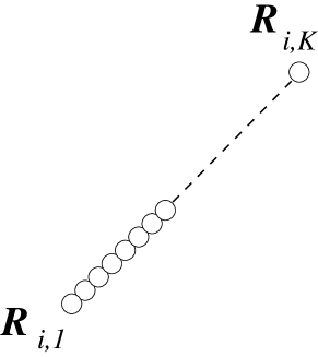
Figure 2: Shish kebab model for the bars composing the chain.

In the case of dynamics it is possible to set the diameters of the spheres by choosing their diffusion constants (or alternatively their mobility, their relaxation times etc.) appropriately. Here we will assume that the diffusion constant is given by $D=\frac{k_{B}T}{3\pi\eta\Delta l}$, where $\eta$ is the viscosity of the medium in which the chain fluctuates. This choice corresponds to spheres of diameter $\Delta l$. It does not reduce the generality of our discussion, which remains valid in the case of any other choice. The positions of the centers of mass of the $k-$th sphere belonging to the $i-$th shish-kebab is described by the radius vectors $\bm{R}_{i,k}$, $i=1,\ldots,N$ and $k=1,\ldots,K$. Throughout the rest of this Section the words shish-kebab and bar will be used interchangeably despite the fact that they are related to different objects. In the next Section we will see that one-dimensional bars are recovered in the limit $K\to+\infty$.

At this point we are ready to impose the constraints that fix the positions of the spheres in such a way that their motion will not destroy the shape of the FJBC. First of all, we need to derive the set of conditions satisfied by the spheres belonging to the same bar. To this purpose we note that if two spheres $k$ and $k^{\prime}$ belong to the same $i-$th bar, the distance between their centers of mass must be $\frac{a}{K}|k-k^{\prime}|$. As a consequence, the radius vectors $\bm{R}_{i,k}$ and $\bm{R}_{i,k^{\prime}}$ have to satisfy the relations:

$$\left|\bm{R}_{i,k^{\prime}}(t)-\bm{R}_{i,k}(t)\right|=\frac{a}{K}|k-k^{\prime}|\qquad k\neq k^{\prime}\qquad k,k^{\prime}=1,\ldots,K$$ (68)

The above set of constraints is sufficient in order to guarantee that the spheres in a bar will remain aligned during their fluctuations.

Next, we have to be sure that the ends of the bars are correctly connected together in order to form a chain. This goal is realized by identifying the $K-$th sphere of the $i-$th bar with the first sphere of the $(i+1)-$th bar, see Fig. 3.

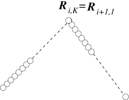
Figure 3: This figure shows how the bars are connected together to build the FJBC.

This requirement implies that the locations of the centers of mass of the spheres should be constrained by the conditions:

$$\bm{R}_{i,K}=\bm{R}_{i+1,1}\qquad i=1,\ldots,N-1$$ (69)

Let us note that $\bm{R}_{1,1}$ and $\bm{R}_{N,K}$ are not affected by the constraints (69) because they are at the ends of the chain which are free.

Before continuing our main discussion, let’s make a digression concerning the length of the FJBC defined above. The total length of the chain is not $L=Na$, because we have to subtract from this value the length $\Delta l(N-1)$ of the $N$ spheres which are identified at the joints. After doing that, we obtain the effective length $\tilde{L}$ of the chain:

$$\tilde{L}=Na-\Delta l(N-1)$$ (70)

Due to the fact that $\Delta l=\frac{a}{K}$, we get:

$$\tilde{L}=\frac{a(K-1)N}{K}+\frac{a}{K}$$ (71)

Let us now come back to the constraints (68) and (69). They represent all the constraints that are needed to make sure that the shape of the $FJBC$ is preserved during the motion of the spheres. Luckily, the constraints (69) may be easily eliminated. This fact was already noted in Ref. [5] and is one of the main advantages to construct an inextensible chains starting from a set of rigid and inextensible basic units. In order to get rid of the conditions (69), we choose as independent coordinates the radius vectors $\bm{R}_{i+1,1}$’s. Accordingly, the radius vectors $\bm{R}_{i,K}$’s have to be replaced everywhere with the $\bm{R}_{i+1,1}$’s. First of all, we have to perform the substitutions $\bm{R}_{i,K}\longrightarrow\bm{R}_{i+1,1}$ inside the relations (68). In order to proceed, it is convenient to divide these relations into three sets. The first set imposes conditions only on the coordinates $\bm{R}_{i,k}$ for $i=1,\ldots,N$ and $k=1,\ldots,K-1$. These coordinates are not located at the junctions between two neighboring bars and thus are not affected by the elimination of the constraints (69). As a consequence, in the restricted range of the indexes for which $i=1,\ldots,N$ and $k\neq k^{\prime}=1,\ldots,K-1$, we can simply rewrite the constraints (68) without changes:

$$\left|\bm{R}_{i,k^{\prime}}-\bm{R}_{i,k}\right|=\frac{a}{K}|k-k^{\prime}|\qquad k\neq k^{\prime}\qquad k\neq k^{\prime}=1,\ldots,K-1\qquad i=1,\ldots,N$$ (72)

Let’s consider now Eq. (68) for $k^{\prime}=K$, $k=1,\ldots,K-1$ and $i=1,\ldots,N-1$. This set of conditions contains the coordinates $\bm{R}_{i,K}$ for $i=1,\ldots,N-1$. They should be substituted by the variables $\bm{R}_{i+1,1}$’s as mentioned above. This operation results in the new conditions:

$$\left|\bm{R}_{i+1,1}-\bm{R}_{i,k}\right|=\frac{a}{K}|K-k|\qquad i=1,\ldots,N-1\qquad k=1,\ldots,K-1$$ (73)

At this point, we are left only with the subset of equations (68) which is strictly related to the spheres of the $N-$th bar. Clearly, the $K-$th sphere in the $N-$th bar is on one of the two free ends of the chain. Thus, it is not constrained by Eq. (69) and the constraints of Eq. (68) should not be changed in this case:

$$\left|\bm{R}_{N,K}-\bm{R}_{N,k}\right|=\frac{a}{K}|K-k|\qquad k=1,\ldots,K-1$$ (74)

We are now ready to proceed with the construction of the generating functional of the FJBC. Exactly as we did for the FHC, we first introduce the Langevin equations that describe the fluctuations of the spheres. In the present situation the number of spheres is $KN$. Their positions are denoted by the vectors $R_{i,k}$, where $i=1,\ldots,N$ and $k=1,\ldots,K$. Accordingly, we have to introduce a set of $KN$ Langevin equations:

$$\bm{\dot{R}}_{i,k}(t)=\bm{\nu}_{i,k}{\normalsize(t)}\qquad i=1,\ldots,N\qquad k=1,\ldots,K$$ (75)

In analogy with the case of the FHC, the probability distributions of the noises $\bm{\nu}_{i,k}$’s are nonlinear as a consequence of the constraints of Eqs. (72–74). Before giving the explicit expressions of these distributions, however, we have to impose in equations (75) the constraints (69). Due to these constraints, in fact, not all the random forces appearing in Eq. (75) are independent. Indeed, using the relations (69) it is easy to check that:

$$\bm{\nu}_{i,K}=\bm{\nu}_{i+1,1}\qquad i=1,\ldots,N-1$$ (76)

The above equations have a very simple physical explanation. In order to join the bars together, some of the spheres have been identified. As a result, the spheres identified in this way are also subjected to the same noise and thus Eqs. (76) should be satisfied. In a similar way as we did for the constraints (68), we may easily get rid of the redundant noises $\bm{\nu}_{i,K}$, $i=1,\ldots,N-1$ from the Langevin equations (75) at the price of dividing these equations into two sets. In the first set there will be only the spheres with indexes $k<K$:

$$\bm{\dot{R}}_{i,k}=\bm{\nu}_{i,k}\qquad i=1,\ldots,N\qquad k=1,\ldots,K-1$$ (77)

The degrees of freedom $\bm{R}_{i,K}$ and $\bm{\nu}_{i,K}$ for $i=1,\ldots,N-1$ are spurious due to the constraints (69) and (76), so that they should not be taken into account. It remains only to consider the fluctuations of the last sphere on the last bar corresponding to the indexes $i=N$ and $k=K$. This sphere is not constrained because it is located at one free end of the chain. The related Langevin equation reads as follows:

$$\bm{\dot{R}}_{N,K}=\bm{\nu}_{N,K}$$ (78)

There are no other independent Langevin equations besides Eqs. (77) and (78).

Having eliminated the constraints (69), we are ready to construct the generating functional of the FJBC. Let us note that the remaining constraints are imposing conditions on the reciprocal distances between two points (the centers of mass of the spheres) exactly as the constraints of the FHC given in Eq. (33) do. As a consequence, it is possible to use the same strategy proposed in Subsection 3.1 in order to fix the conditions of Eqs. (72–74). Accordingly, we introduce the following non-gaussian noise distribution:

$$\mathcal{D}\rho(\{\bm{\nu}_{i,k}\}) = \left[\prod_{i=1}^{N}\prod_{k=1}^{K-1}\mathcal{D}\bm{\nu}_{i,k}\right]{\cal D}\bm{\nu}_{N,K}\exp\left[-\frac{1}{4D}\sum_{i=1}^{N}\sum_{k=1}^{K-1}\int_{0}^{t_{f}}\bm{\nu}_{i,k}^{2}dt\right]$$ (79)

$$\times \exp\left[-\frac{1}{4D}\int_{0}^{t_{f}}\bm{\nu}_{N,K}^{2}dt\right]e^{-\tilde{W}(\{\bm{R}_{i,k,\bm{\nu}_{i,k}}\},\beta_{1},\beta_{2},\beta_{3})}$$

The potential $\tilde{W}(\{\bm{R}_{i,k,\bm{\nu}_{i,k}}\},\beta_{1},\beta_{2},\beta_{3})$ is a function of the solutions $\{\bm{R}_{i,k,\bm{\nu}_{i,k}}\}$ of Eqs. (77–78) and thus of the noises $\bm{\nu}_{i,k}$ for $i=1,\ldots,N-1$ and $k=1,\ldots,K-1$ and $\bm{\nu}_{N,K}$. The form of $\tilde{W}$ can be chosen following the same criteria 1. – 3. discussed in Subsection 3.1. A slight difference from the FHC is that, due to the splitting of the constraints (68) into the three sets of equations given in (72–74), the FJBC potential $\tilde{W}(\{\bm{R}_{i,k,\bm{\nu}_{i,k}}\},\beta_{1},\beta_{2},\beta_{3})$ will depend on three parameters $\beta_{1},\beta_{2}$ and $\beta_{3}$ instead of one. The underlying idea is however the same. When these parameters approach infinity, $\tilde{W}(\{\bm{R}_{i,k,\bm{\nu}_{i,k}}\},\beta_{1},\beta_{2},\beta_{3})$ should be chosen in such a way that it becomes infinite outside the region in the coordinate space in which the constraints (72–74) are satisfied and zero otherwise. Let’s now derive $\tilde{W}(\{\bm{R}_{i,k,\bm{\nu}_{i,k}}\},\beta_{1},\beta_{2},\beta_{3})$ explicitly. We have to require that the solutions $\bm{R}_{i,k,\bm{\nu}_{i,k}}$ of the Langevin equations (77) and (78) satisfy the constraints (72–74). We recall that the $\bm{R}_{i,k,\bm{\nu}_{i,k}}$’s are purely functions of the noises $\nu_{i,k}$, so that the relations (72–74) are conditions on the noise degrees of freedom. Moreover, Eqs. (72–74) are of the form:

$$\bm{R}_{a}-\bm{R}_{b}=d_{ab}$$ (80)

In other words, as previously stressed, they constrain the distance between two points $a$ i $b$ exactly as the constraints of the FHC of Eq. (35). In order to implement constraints of this kind we can imagine, as it has been done in the previous Subsection, that the two points $a$ and $b$ are connected together by a spring with rest length $d_{ab}>0$. In the limit of infinite elastic constant, the spring is frozen in its rest position and the distance between the points is fixed to $d_{ab}$. These consideration suggest that constraints of the kind given in Eq. (80) may be fixed using the elastic potential

$$V_{ab}(|\bm{R}_{a}-\bm{R}_{b}|)=\frac{\beta}{2}\left(|\bm{R}_{a}-\bm{R}_{b}|-d_{ab}\right)^{2}$$ (81)

There is however no reason for restricting ourselves to elastic interactions. Any two-body interaction that freezes the distance between two points in the limit of infinite strength is suitable. Of course, the related potential should have an infinitely sharp peak in the region for which $|\bm{R}_{a}-\bm{R}_{b}|=d_{ab}$. Moreover, it has to be of the form $V(|\bm{R}_{a}-\bm{R}_{b}|)=f^{2}(|\bm{R}_{a}-\bm{R}_{b}|)$, where $f$ is an arbitrary function, otherwise it will no longer be possible to use the identity (60). For example, a valid potential is the following:

$$V^{\prime}_{ab}|\bm{R}_{a}-\bm{R}_{b}|)=\beta\left(|\bm{R}_{a}-\bm{R}_{b}|^{2}-d^{2}_{ab}\right)^{2}$$ (82)

It is easy to show that the above potential is completely equivalent to the elastic one given in Eq. (81). This becomes clear if we rewrite $V^{\prime}_{ab}(|\bm{R}_{a}-\bm{R}_{b}|)$ in the form

$$V^{\prime}_{ab}(|\bm{R}_{a}-\bm{R}_{b}|)=\beta\left(|\bm{R}_{a}-\bm{R}_{b}|-d_{ab}\right)^{2}\left(|\bm{R}_{a}-\bm{R}_{b}|+d_{ab}\right)^{2}$$ (83)

Of course, the minimum of $V^{\prime}_{ab}(|\bm{R}_{a}-\bm{R}_{b}|$ at $|\bm{R}_{a}-\bm{R}_{b}|+d_{ab}=0$ will never be reached because $d_{ab}>0$. Therefore, exactly as in the case of the elastic potential (81), $V^{\prime}_{ab}(|\bm{R}_{a}-\bm{R}_{b}|)$ imposes only the condition $|\bm{R}_{a}-\bm{R}_{b}|-d_{ab}=0$. Moreover, it is possible to check that $V^{\prime}_{ab}(|\bm{R}_{a}-\bm{R}_{b}|)$ verifies all conditions 1. – 3. of Subsection 3.1. In particular, in the limit $\beta=+\infty$ $V^{\prime}_{ab}(|\bm{R}_{a}-\bm{R}_{b}|)$ is zero if the constraints are satisfied and infinite in the opposite case. The advantage of choosing the potential of Eq. (82) is that it leads directly to a delta function in the desired form $\delta(|\bm{R}_{a}-\bm{R}_{b}|^{2}-d_{ab}^{2})$, so that we do not have to pass through all the intermediate steps performed in Eqs. (62) and (63) in order to arrive at the final generating functional $Z_{FHC}[J]$ of the FHC given in Eq. (64). Taking into account all the above considerations, to implement the constraints of Eqs. (72–74) we will choose the following potentials:

$$V_{i,kk^{\prime}}(\left|\bm{r}_{i,k}-\bm{r}_{i,k^{\prime}}\right|)=(\Delta l)^{2}\beta_{1}\left(\frac{\left|\bm{r}_{i,k}-\bm{r}_{i,k^{\prime}}\right|^{2}}{a^{2}}-\frac{\left|k-k^{\prime}\right|^{2}}{K^{2}}\right)^{2}\qquad\left\{\begin{array}[]{ccc}i&=&1,\ldots,N-1\\ k\neq k^{\prime}&=&1,\ldots,K-1\end{array}\right.$$ (84)

$$V_{i,k}(\left|\bm{r}_{i+1,1}-\bm{r}_{i,k}\right|)=\Delta l\beta_{2}\left(\frac{\left|\bm{r}_{i+1,1}-\bm{r}_{i,k}\right|^{2}}{a^{2}}-\frac{\left|K-k\right|^{2}}{K^{2}}\right)^{2}\qquad\left\{\begin{array}[]{ccc}i&=&1,\ldots,N-1\\ k&=&1,\ldots,K-1\end{array}\right.$$ (85)

$$V_{k}(\left|\bm{r}_{N,K}-\bm{r}_{N,k}\right|)=\Delta l\beta_{3}\left(\frac{\left|\bm{r}_{N,K}-\bm{r}_{N,k}\right|^{2}}{a^{2}}-\frac{\left|K-k\right|^{2}}{K^{2}}\right)^{2}\qquad k=1,\ldots,K-1$$ (86)

Here $\beta_{1}$, $\beta_{2}$, $\beta_{3}$ are real parameters and are supposed to be very large. Eventually, we will take the limit $\beta_{1}$, $\beta_{2}$, $\beta_{3}\rightarrow\infty$. Let us note the change of length scale with respect to the FHC. Here the smallest scale is the distance $\Delta l$ between the centers of mass of two contiguous spheres belonging to the same bar. As a consequence, the analog of Eq. (12) in the present case is:

$$V_{FJBC}(\Delta l)=\sum_{k=1}^{K}\Delta l{\tilde{V}}_{E}(\bm{R}_{i,k}(t))+\sum_{\underset{k\neq k^{\prime}}{k,k^{\prime}=1}}^{K}\Delta l^{2}{\tilde{V}}_{I}(\bm{R}_{i,k}(t),\bm{R}_{j,k^{\prime}}(t))$$ (87)

The above form of the potential guarantees the correct passage to the limit $\Delta l\to 0$ and $K\to+\infty$ in which the bars become continuous and one-dimensional systems with uniform mass distribution. Indeed, it may be easily checked that in this continuous limit Eq. (87) reduces to the potential for a chain of one-dimensional bars with uniform and continuous mass distribution given in Eq. (28).

Going back to the main problem of constructing the generating functional of the FJBC, we define $\tilde{W}(\{R_{i,k}\})$ as the following linear combination of the potentials (84–86):

$$\tilde{W}(\{r_{i,k}\}) = \sum_{i=1}^{N}\sum_{k,k^{\prime}=1\atop k\neq k^{\prime}}^{K-1}\int_{0}^{t_{f}}\left[V_{i,kk^{\prime}}(\left|\bm{r}_{i,k}-\bm{r}_{i,k^{\prime}}\right|)+\sum_{i=1}^{N-1}\sum_{k=1}^{K-1}V_{i,k}(\left|\bm{r}_{i+1,1}-\bm{r}_{i,k}\right|)\right.$$ (88)

$$+ \left.\sum_{k=1}^{K-1}V_{k}(\left|\bm{r}_{N,K}-\bm{r}_{N,k}\right|)\right]dt$$

By substituting the right hand side of Eq. (88) in Eq. (79), we obtain the noise distribution $\mathcal{D}\rho(\{\bm{\nu}_{i,k}\})$. Knowing the noise distribution it is possible to construct the generating functional of the FJBC in path integral form:

$$Z_{FJBC}[J] =\lim_{\beta_{1},\beta_{2},\beta_{3}\to+\infty}\left[\prod_{i=1}^{N}\prod_{k=1}^{K-1}\int\mathcal{D}\bm{\nu}_{i,k}\right]\exp\left[-\sum_{i=1}^{N}\sum_{k=1}^{K-1}\int_{0}^{t_{f}}\left(\frac{1}{4D}\bm{\nu}_{i,k}^{2}+\Delta l\bm{J}_{i,k}\cdot\bm{R}_{i,k,\bm{\nu}_{i,k}}\right)dt\right]$$

$$\int\mathcal{D}\bm{\nu}_{N,K}\exp\left[-\int_{0}^{t_{f}}\left(\frac{1}{4D}\bm{\nu}_{N,K}^{2}+\Delta l\bm{J}_{N,K}\cdot\bm{R}_{N,K,\bm{\nu}_{N,K}}\right)dt\right]\exp\left[-{\tilde{W}}(\{R_{i,k,\bm{\nu}_{i,k}}\})\right]$$ (89)

At this point, in analogy with the steps (47–49) made in Section 3.1, we insert in the generating functional (89) the quantity:

$$\tilde{I}=\left[\prod_{i=1}^{N}\prod_{k=1}^{K-1}\int\mathcal{D}\bm{r}_{i,k}\delta(\bm{r}_{i,k}-\bm{R}_{i,k,\bm{\nu}_{i,k}})\right]\int\mathcal{D}\bm{r}_{N,K}\delta(\bm{r}_{N,K}-\bm{R}_{N,K,\bm{\nu}_{N,K}})$$ (90)

Clearly $\tilde{I}=1$, so its insertion in Eq. (89) does not change the physics of the problem. It is also possible to check that:

$$\tilde{I}=\left[\prod_{i=1}^{N}\prod_{k=1}^{K-1}\det\left[\frac{\partial}{\partial t}\right]\int\mathcal{D}\bm{r}_{i,k}\delta(\bm{\dot{r}}_{i,k}-\bm{\nu}_{i,k})\right]\det\left[\frac{\partial}{\partial t}\right]\int\mathcal{D}\bm{r}_{N,K}\delta(\bm{\dot{r}}_{N,K}-\bm{\nu}_{N,K})$$ (91)

As a result of the insertion of $\tilde{I}$, we get after an easy integration over the noises $\bm{\nu}_{i,k}$ and $\bm{\nu}_{N,K}$:

$$Z_{FJBC}[J] = \lim_{\beta_{1},\beta_{2},\beta_{3}\to+\infty}\left[\prod_{i=1}^{N}\prod_{k=1}^{K-1}\int\mathcal{D}\bm{r}_{i,k}\right]\exp\left[-\sum_{i=1}^{N}\sum_{k,k^{\prime}=1\atop k\neq k^{\prime}}^{K-1}\int_{0}^{t_{f}}\left(\frac{1}{4D}\bm{\dot{r}}_{i,k}^{2}+\Delta l\bm{J}_{i,k}\cdot\bm{r}_{i,k}\right)dt\right]$$ (92)

$$\times \int\mathcal{D}\bm{r}_{N,K}\exp\left[-\int_{0}^{t_{f}}\left(\frac{1}{4D}\bm{\dot{r}}_{N,K}^{2}dt+\Delta l\bm{J}_{N,K}\cdot\bm{r}_{N,K}\right)dt\right]$$

$$\times \exp\left[-(\Delta l)^{2}\beta_{1}\sum_{i=1}^{N}\sum_{k,k^{\prime}=1\atop k\neq k^{\prime}}^{K-1}\int_{0}^{t_{f}}\left(\frac{\left|\bm{r}_{i,k}-\bm{r}_{i,k^{\prime}}\right|^{2}}{a^{2}}-\frac{\left|k-k^{\prime}\right|^{2}}{K^{2}}\right)^{2}dt\right]$$

$$\times \exp\left[-\Delta l\beta_{2}\sum_{i=1}^{N-1}\sum_{k=1}^{K-1}\int_{0}^{t_{f}}\left(\frac{\left|\bm{r}_{i+1,1}-\bm{r}_{i,k}\right|^{2}}{a^{2}}-\frac{\left|K-k\right|^{2}}{K^{2}}\right)^{2}dt\right]$$

$$\times \exp\left[-\Delta l\beta_{3}\sum_{k=1}^{K-1}\int_{0}^{t_{f}}\left(\frac{\left|\bm{r}_{N,K}-\bm{r}_{N,k}\right|^{2}}{a^{2}}-\frac{\left|K-k\right|^{2}}{K^{2}}\right)^{2}dt\right]$$

Finally, we apply Eq. (60) in order to perform the limits $\beta_{1}$, $\beta_{2}$, $\beta_{3}\rightarrow+\infty$. The result is:

$$Z_{FJBC}[J] = \left[\prod_{i=1}^{N}\prod_{k=1}^{K-1}\int\mathcal{D}\bm{r}_{i,k}\right]\exp\left[-\sum_{i=1}^{N}\sum_{k,k^{\prime}=1\atop k\neq k^{\prime}}^{K-1}\int_{0}^{t_{f}}\left(\frac{1}{4D}\bm{\dot{r}}_{i,k}^{2}+\Delta l\bm{J}_{i,k}\cdot\bm{r}_{i,k}\right)dt\right]$$ (93)

$$\times \int\mathcal{D}\bm{r}_{N,K}\exp\left[-\int_{0}^{t_{f}}\left(\frac{1}{4D}\bm{\dot{r}}_{N,K}^{2}dt+\Delta l\bm{J}_{N,K}\cdot\bm{r}_{N,K}\right)dt\right]$$

$$\times \left[\prod\limits_{i=1}^{N}\prod\limits_{\begin{subarray}{c}k,k^{\prime}=1\\ k\neq k^{\prime}\end{subarray}}^{K-1}\delta\left(\frac{\left|\bm{r}_{i,k}-\bm{r}_{i,k^{\prime}}\right|^{2}}{a^{2}}-\frac{\left|k-k^{\prime}\right|^{2}}{K^{2}}\right)\right]$$

$$\times \left[\prod\limits_{i=1}^{N-1}\prod\limits_{k=1}^{K-1}\delta\left(\frac{\left|\bm{r}_{i+1,1}-\bm{r}_{i,k}\right|^{2}}{a^{2}}-\frac{\left|K-k\right|^{2}}{K^{2}}\right)\right]$$

$$\times \left[\prod\limits_{k=1}^{K-1}\delta\left(\frac{\left|\bm{r}_{N,K}-\bm{r}_{N,k}\right|^{2}}{a^{2}}-\frac{\left|K-k\right|^{2}}{K^{2}}\right)\right]$$

This is the expression of the generating functional of the discrete FJBC in the shish kebab approximation.

4 The double continuous limit of the FJBC

Before performing the continuous limit of the generating functional (93), it is important to recall how the FJBC is constructed. The FJBC consists in one-dimensional systems with an uniform and continuous distribution of mass as it was explained when discussing the classical case and in Subsection 3.2. In our approach each bar has been approximated by a shish-kebab model, in which $K$ small spheres are put together in a row by imposing the constraints (72–74). The distance between the centers of mass of the spheres is given by the quantity $\Delta l$ of Eq. (67). One can see the spheres as small masses $m$ localized at regular intervals on a segment of length $a$. The three dimensionality of the spheres is adjusted by tuning the diffusion constant $D$. In the present case $D$ has been choosen in such a way that it coincides with the diffusion constant of a small sphere of diameter $\Delta l$. Of course, if the length $a$ of the bar is finite, the more spheres we will use, the better will be the approximation of the bar. To reproduce the FJBC, an infinite number of spheres is necessary. Indeed, when $K$ is infinite, the diameter of the spheres approaches zero as it is shown by Eq. (67) and the shish-kebab models coincides with an uniform distribution of point-like masses distributed on a segment of length $a$. This is exactly the one-dimensional bar that has been taken as the basic unit in the FJBC model.

As a warming up exercise, the probability function of the FJBC will be computed in the limit $\Delta l\to 0$ and $K\to+\infty$. As explained before, this limit corresponds to the one-dimensional chain with uniform mass distribution without the shish-kebab approximation. In that limit $\tilde{L}$ and $L$ coincide and the length of each bar will be equal to $a$ because the decrease of the length due to the way in which the bars are joined together becomes negligible when $\Delta l\to 0$ and $K\to+\infty$.

First of all, we derive the expression of the mass $m$ of a single sphere in terms of two macroscopic parameters, namely the total length of the chain $\tilde{L}$ and its total mass $M$. To compute $M$, we subtract from the total mass $NKm$ of $N$ bars the mass $(N-1)m$ of the $N-1$ spheres which disappear because they are identified at the junctions between the bars. The result is $M=NKm-(N-1)m$, Thus we may write:

$$m=\frac{M}{N(K-1)+1}$$ (94)

Using Eq. (71), we get:

$$m=\frac{Ma}{K\tilde{L}}=\frac{M}{\tilde{L}}\Delta l$$ (95)

where $\frac{M}{\tilde{L}}$ is the uniform mass density. The analog of Eq. (66) in the FJBC case is:

$$\frac{1}{4D}=\frac{1}{2kT\tau}\frac{M}{2{\tilde{L}}}\Delta l$$ (96)

Next, we provide the prescriptions to pass to the continuous bar limit $\Delta l\to 0$ and $K\to+\infty$:

$$\sum_{k=1}^{K-1}\Delta l\to\int_{0}^{a}dl \sum_{k,k^{\prime}=1}^{K-1}(\Delta l)^{2}\to\int_{0}^{a}dldl^{\prime}$$ (97)

$$\bm{r}_{i,k}(t)\to\bm{r}_{i}(t,l) {\tilde{L}}\to L$$ (98)

$$\bm{r}_{i}(t,0)=\bm{r}_{i,1}(t) \bm{r}_{i}(t,a)=\bm{r}_{i+1,1}(t)$$ (99)

$$a\frac{k}{K}\to l$$ (100)

Using the above formulas (96–100) is is not difficult to show that:

$$Z_{FJBC}^{K=\infty}[J] = \lim_{\beta_{1},\beta_{2},\beta_{3}\to+\infty}\left[\prod_{i=1}^{N}\int{\cal D}\bm{r}_{i}(t,l)\right]\exp\left[-\sum_{i=1}^{N}\int_{0}^{t_{f}}dtI_{i}^{(0)}(t)\right]$$ (101)

$$\times \exp\left[-\beta_{1}\sum_{i=1}^{N}\int_{0}^{t_{f}}dtI_{i}^{(1)}(t)\right]\exp\left[-\beta_{2}\sum_{i=1}^{N-1}\int_{0}^{t_{f}}dtI_{i}^{(2)}(t)\right]$$

$$\times \exp\left[-\beta_{3}\int_{0}^{t_{f}}dtI_{i}^{(3)}(t)\right]$$

where

$$I_{i}^{(0)}(t)=\int_{0}^{a}dl\left(\frac{1}{2kT\tau}\frac{M}{2L}\dot{\bm{r}}_{i}^{2}(t,l)+\bm{J}_{i}(t,l)\cdot\bm{r}_{i}(t,l)\right)$$ (102)

$$I_{i}^{(1)}(t)=\int_{0}^{a}dldl^{\prime}\left(\frac{|\bm{r}_{i}(t,l)-\bm{r}_{i}(t,l^{\prime})|^{2}}{a^{2}}-\frac{|l-l^{\prime}|^{2}}{a^{2}}\right)^{2}$$ (103)

$$I_{i}^{(2)}(t)=\int_{0}^{a}dl\left(\frac{|\bm{r}_{i+1}(t,0)-\bm{r}_{i}(t,l)|^{2}}{a^{2}}-\frac{|a-l|^{2}}{a^{2}}\right)^{2}$$ (104)

$$I_{N}^{(3)}(t)=\int_{0}^{a}dl\left(\frac{|\bm{r}_{N}(t,a)-\bm{r}_{N}(t,l)|^{2}}{a^{2}}-\frac{|a-l|^{2}}{a^{2}}\right)^{2}$$ (105)

By taking the limit $\beta_{1},\beta_{2},\beta_{3}\to+\infty$ we finally obtain the probability function of the FJBC:

$$Z_{FJBC}^{K=\infty}[J] = \left[\prod_{i=1}^{N}\int{\cal D}\bm{r}_{i}(t,l)\right]\exp\left[-\sum_{i=1}^{N}\int_{0}^{t_{f}}dt\int_{0}^{a}dl\left(\frac{1}{2kT\tau}\frac{M}{2L}\dot{\bm{r}}_{i}^{2}(t,l)+\bm{J}_{i}(t,l)\cdot\bm{r}_{i}(t,l)\right)\right]$$ (106)

$$\times \left[\prod_{i=1}^{N}\delta\left(\frac{|\bm{r}_{i}(t,l)-\bm{r}_{i}(t,l^{\prime})|^{2}}{a^{2}}-\frac{|l-l^{\prime}|^{2}}{a^{2}}\right)\right]\left[\prod_{i=1}^{N-1}\delta\left(\frac{|\bm{r}_{i+1,1}(t)-\bm{r}_{i}(t,l)|^{2}}{a^{2}}-\frac{|a-l|^{2}}{a^{2}}\right)\right]$$

$$\times \delta\left(\frac{|\bm{r}_{N}(t,a)-\bm{r}_{N}(t,l)|^{2}}{a^{2}}-\frac{|a-l|^{2}}{a^{2}}\right)$$

We would like to check if, in the limit of a continuous chain (6), the generating functional of the FJBC reduces to the partition function of the GNL$\sigma$M of Eq. (65) as it should be expected. Our starting point will be the generating functional $Z_{FJBC}^{K=\infty}[J]$ in the version of Eq. (101). First of all we expand the functions $I_{i}^{(0)}(t),\ldots,I_{N}^{(3)}(t)$ given in Eqs. (102–105) at the leading order in $a$. Since at the end the limit $a\to 0$ will be taken, there is no need to compute higher order terms. A straightforward application of the expansion in Taylor series gives for $I_{i}^{(0)}(t)$:

$$I_{i}^{(0)}(t)=\left(\frac{1}{2kT\tau}\frac{M}{2L}\dot{\bm{r}}^{2}_{i,1}(t)+\bm{J}_{i,1}(t)\cdot\bm{r}_{i,1}(t)\right)a$$ (107)

To write down the above equation we have used the prescription (99) according to which $\bm{r}_{i}(t,0)=\bm{r}_{i,1}(t)$. Let us consider now the term $I_{i}^{(1)}(t)x$. Due to the fact that we are working in the region of small values of $a$, it is possible to make the following approximation:

$$\left|\frac{\bm{r}_{i}(t,l)-\bm{r}_{i}(t,l^{\prime})}{l-l^{\prime}}\right|\sim\left|\frac{\bm{r}_{i}(t,a)-\bm{r}_{i}(t,a)}{a}\right|$$ (108)

Both members of the above equation coincide in fact with the modulus of the derivative $\left|\frac{\partial\bm{r}_{i}(t,0)}{\partial l}\right|$ up to higher order terms in the infinitesimal quantities $l,l^{\prime}$ and $a$. Using Eq. (108) to simplify the expression of $I_{i}^{(1)}(t)$ given in (103), we obtain:

$$I_{i}^{(1)}(t)\sim\left\{\begin{array}[]{cc}\left(\frac{|\bm{r}_{i+1,1}(t)-\bm{r}_{i,1}(t)|^{2}}{a^{2}}-1\right)^{2}A&\mbox{for $i=1,\ldots,N-1$}\\ \left(\frac{|\bm{r}_{N}(t,a)-\bm{r}_{N}(t,0)|^{2}}{a^{2}}-1\right)^{2}A&\mbox{for $i=N$}\end{array}\right.$$ (109)

where $A=\int_{0}^{a}dldl^{\prime}\frac{|l-l^{\prime}|^{4}}{a^{4}}$. A direct calculation shows that:

$$A=\frac{a^{2}}{15}$$ (110)

Similar calculations allow the computation of $I_{i}^{(2)}(t)$ and $I_{N}^{(3)}(t)$:

$$I_{i}^{(2)}(t)\sim\left(\frac{|\bm{r}_{i+1,1}(t)-\bm{r}_{i,1}(t)|^{2}}{a^{2}}-1\right)^{2}\frac{a}{5}\qquad\qquad i=1,\ldots,N-1$$ (111)

$$I_{N}^{(3)}(t)\sim\left(\frac{|\bm{r}_{N}(t,a)-\bm{r}_{N}(t,0)|^{2}}{a^{2}}-1\right)^{2}\frac{a}{5}$$ (112)

As we see from Eqs. (107–112), in the action of the generating functional $Z_{FJBC}^{K=\infty}[J]$ many degrees of freedom disappear when $a$ becomes small. The only remaining degrees of freedom are the variables $\bm{r}_{i,1}(t)=\bm{r}_{i}(t,0)$ for $i=1,\ldots,N$ and $\bm{r}_{N}(t,a)$. All the other degrees of freedom $\bm{r}_{i}(t,l)$ for $l\neq 0$ and $l\neq a$ can be simply integrated out in Eq. (101), because they do not appear in the functions $I_{i}^{(0)}(t),\ldots,I_{N}^{(3)}(t)$ of Eqs. (102–105) and thus in the generating functional $Z_{FJBC}^{K=\infty}[J]$. Their integration will result in a constant overall factor $\cal C$ multiplied with the rest of the generating functional. Moreover, when $a$ goes to zero, all terms containing positive powers of $a$ vanish identically if these powers are not absorbed by an appropriate number of sums over all bars according to the prescription $\sum_{i=1}^{N}a\to\int_{0}^{L}ds$. In particular it is easy to check that

$$\lim_{a\to 0}\sum_{i=1}^{N}\int_{0}^{t_{f}}dtI_{i}^{(1)}=0$$ (113)

and

$$\lim_{a\to 0}\int_{0}^{t_{f}}dtI_{N}^{(3)}=0$$ (114)

As a consequence, for small values of $a$ the leading order contribution to the generating functional $Z_{FJBC}^{K=\infty}[J]$ is provided by:

$$Z_{FJBC}^{K=\infty}[J] \sim \lim_{\beta_{2}\to+\infty}{\cal C}\left[\prod_{i=1}^{N}\int{\cal D}\bm{r}_{i,1}(t)\right]\exp\left[-\sum_{i=1}^{N}a\int\limits_{0}^{t_{f}}dt\left(\textstyle\frac{1}{2kT\tau}\frac{M}{2L}\dot{\bm{r}}^{2}_{i,1}(t)+\bm{J}_{i,1}(t)\cdot\bm{r}_{i,1}(t)\right)\right]$$ (115)

$$\times \exp\left[-\frac{\beta_{2}}{5}\sum_{i=1}^{N-1}a\int_{0}^{t_{f}}dt\left(\frac{|\bm{r}_{i+1,1}(t)-\bm{r}_{i,1}(t)|^{2}}{a^{2}}-1\right)^{2}\right]$$

Now it is possible to proceed with the continuous limit (6) following the prescription of Subsection 2.1. The result is:

$$\lim_{a\to 0,N\to+\infty,Na=L}Z_{FJBC}^{K=\infty}[J]=Z^{\prime}[J]$$ (116)

where

$$Z^{\prime}[J] = \lim_{\beta_{2}\to+\infty}{\cal C}\int{\cal D}\bm{r}(t,s)\exp\left[-\int_{0}^{t_{f}}dt\int_{0}^{L}ds\left(\textstyle\frac{1}{2kT\tau}\frac{M}{2L}\dot{\bm{r}}^{2}(t,s)+\bm{J}(t,s)\cdot\bm{r}(t,s)\right)\right]$$ (117)

$$\times \exp\left[-\frac{\beta_{2}}{5}\int_{0}^{t_{f}}dt\int_{0}^{L}ds\left(\left|\frac{\partial\bm{r}(t,s)}{\partial s}\right|^{2}-1\right)^{2}\right]$$

Performing also the limit for infinitely large values of $\beta_{2}$, we obtain up to an irrelevant proportionality constant:

$$Z^{\prime}[J] = \int{\cal D}\bm{r}(t,s)\exp\left[-\int_{0}^{t_{f}}dt\int_{0}^{L}ds\left(\textstyle\frac{1}{2kT\tau}\frac{M}{2L}\dot{\bm{r}}^{2}(t,s)+\bm{J}(t,s)\cdot\bm{r}(t,s)\right)\right]$$ (118)

$$\times \delta\left(\left|\frac{\partial\bm{r}(t,s)}{\partial s}\right|^{2}-1\right)$$

This is exactly the partition function of the GNL$\sigma$M of Eq. (65) as expected.

5 Conclusions

In this work an approach to the dynamics of an inextensible chain has been proposed. At the basis of that approach there is the observation that in a constrained mechanical system fluctuating in some viscous medium at constant temperature, the random noise acting on the system is subjected to constraints too. Following this simple observation, the constraints have been imposed here directly on the noise degrees of freedom. In this way the complications of having to deal with an extended set of degrees of freedom (the Lagrange multipliers) or with generalized coordinates, are absent. In the generating functional of the FHC introduced in Eq. (46), the constraints have been fixed by means of potentials. We recall at this point that even in the case in which the strength of the potentials imposing the inextensibility constraints are very large, numerical simulations show that the fast modes related to the changes of the lengths of the basic units still dominate over the slow modes associated to the conformational changes of the chain [5, 21]. To eliminate this problem, in the generating functional of the FHC the limit in which the strengths of the potential (44) becomes infinite has been performed. The final expression of the generating functional of the FHC in this limit is shown in Eq. (64).

In this work it has also been explored the strategy of Ref. [5], in which it has been proposed that an inextensible chain may be realized gluing together a set of inextensible basic units like for instance one-dimensional bars with uniform mass distribution. In Subsection 3.2 this strategy has been explored for a chain in which the bars have been replaced by the shish-kebabs displayed in Fig. 2. Each shish-kebab consists of $K$ spheres that are aligned together in a row by means of suitable constraints in order to form the approximate shape of a bar. The final expression of the generating functional $Z_{FJBC}[J]$ for this type of chain may be found in Eq. (93). In the limit in which the distance $\Delta l$ between the centers of mass of the spheres vanishes identically and the number $K$ of spheres becomes infinitely large while the product $K\Delta l$ remains finite, the shish-kebabs become one-dimensional bars and one obtains the model of a chain which has been called here FJBC. Its generating functional in path integral form has been given in Eq. (106). As a check of the consistency of our approach it has been verified that in the limit of a continuous chain both generating functionals of the FHC and FJBC coincide. Indeed, after performing the continuous limit, one obtains respectively the generating functionals of Eqs. (65) and (118) that describe the same theory, namely the GNL$\sigma$M of Ref. [29]. The consistency of the approach presented in this work in order to tackle the problem of the dynamics of an inextensible chain is also confirmed by the results of Ref. [32]. In has been shown there that the generating functional of the FHC given in Eq. (64) consists of a statistical sum over all particle trajectories that satisfy the Langevin equations (32) together with the inextensibility constraints (33) as it is expected. In [30] it has been verified that in the continuous case the statistical sum in the GNL$\sigma$M contains only the chain conformations for which $\dot{\bm{R}}(t,s)=\bm{\nu}(t,s)$ and $\left|\partial\bm{R}(t,s)/\partial s\right|=1$. These equations are respectively the continuous counterparts of Eqs. (32) and (33). Additionally, we have explored in this work the Fokker-Planck formulation of the dynamics of the FHC in Eqs. (55)–(59).

Finally, let us mention some issues that are still open. First of all, the hydrodynamic and self-avoiding forces are missing in our approach. To describe the dynamics of realistic chains these interactions should be taken into account. For this reason, up to now the applications of the GNL$\sigma$M are limited to situations in which the speed of the elements of the chain is low, so that the hydrodynamics interactions can be neglected. Let us note that the addition of nonlinear self-interactions acting on the beads of a set of coupled oscillators like that described by Eq. (50) leads to interesting phenomena as described in Refs. [39, 40, 41], where such kind of systems has been studied. Another important issue is to find suitable approximations that may be used to evaluate field path integrals in the presence of functional Dirac delta functions and nontrivial boundary conditions. This is exactly the case of the generating functional of Eq. (65). So far, the partition function and the so-called dynamic structure factor have been derived in the semiclassical approximation [29, 30]. One could simplify the theory even further if it would be possible to extend the well known approximation of the Dirac delta function with a gaussian function also to the functional Dirac delta function imposing the inextensible constraints in the GNL$\sigma$M. At the moment, this extension has been achieved only in the case of the statistical mechanics of the FHC [26]. The generalization of this result to dynamics is still work in progress.

6 Acknowledgments

One of the authors, F. F., is indebted to H. Arodź, Z. Jaskólski, J. Paturej, M. Pia̧tek, V. G. Rostiashvili and T. A. Vilgis for fruitful discussions. This research was supported in part by the National Science Foundation under Grant No. NSF PHY05-51164.

Appendix A – Proof of Eq. (60)

We start from the quantity

$$A(\beta)=C(\beta)\exp\left[-a\beta\int_{0}^{t_{f}}dtf^{2}(\bm{r}_{i}(t),\bm{r}_{j}(t))\right]\qquad\qquad i,j=1,\ldots,N$$ (119)

where $C(\beta)$ is a normalization constant. We discretize the interval of time $[0,t_{f}]$ into $M$ smaller intervals of length $b$. Of course, $Mb=t_{f}$. $A(\beta)$ is recovered in the continuous limit $b\longrightarrow 0$ and $M\longrightarrow+\infty$:

$$A(\beta)=\lim_{\underset{M\to+\infty}{b\to 0}}C_{M}(\beta)\exp\left[-a\beta\sum_{m=1}^{M}bf^{2}(\bm{r}_{i}(t_{m}),\bm{r}_{j}(t_{m})\right]$$ (120)

Here $t_{m}=mb$ is the discretized time variable and $C(\beta)=\lim_{\underset{M\to+\infty}{b\to 0}}C_{M}(\beta)$. Let us put

$$\frac{1}{\epsilon}=a\beta b$$ (121)

and

$$C_{M}(\beta)=\prod_{m=1}^{M}\frac{1}{(4\pi\epsilon)^{\frac{1}{2}}}$$ (122)

Thus

$$A(\beta)=\lim_{\underset{M\to+\infty}{b\to 0}}\left[\prod_{m=1}^{M}\frac{1}{(4\pi\epsilon)^{\frac{1}{2}}}\exp{\left(-\frac{f^{2}(\bm{r}_{i}(t_{m}),\bm{r}_{j}(t_{m}))}{\epsilon}\right)}\right]$$ (123)

We consider at this point the limit $\beta\longrightarrow+\infty$ of $A(\beta)$:

$$\lim_{\beta\to+\infty}A(\beta)=\lim_{\epsilon\to 0}\lim_{\underset{M\to+\infty}{b\to 0}}\left[\prod_{m=1}^{M}\frac{1}{(4\pi\epsilon)^{\frac{1}{2}}}\exp{\left(-\frac{f^{2}(\bm{r}_{i}(t_{m}),\bm{r}_{j}(t_{m}))}{\epsilon}\right)}\right]$$ (124)

Permuting the limit $\epsilon\to 0$ with the limit $M\to+\infty$ and $b\to 0$, we get:

$$\lim_{\beta\to+\infty}A(\beta)=\lim_{\underset{M\to+\infty}{b\to 0}}\left[\prod_{m=1}^{M}\lim_{\epsilon\to 0}\frac{1}{(4\pi\epsilon)^{\frac{1}{2}}}\exp{\left(-\frac{f^{2}(\bm{r}_{i}(t_{m}),\bm{r}_{j}(t_{m}))}{\epsilon}\right)}\right]$$ (125)

When $\beta$ starts to be very large and simultaneously $\epsilon$ becomes very small, it is possible to use the Gaussian representation of the Dirac delta function $\delta(x)=\lim_{\epsilon\to 0}\frac{1}{(4\pi\epsilon)^{\frac{1}{2}}}e^{-\frac{x^{2}}{\epsilon}}$ and to write:

$$\lim_{\beta\to+\infty}A(\beta)=\lim_{\underset{M\to+\infty}{b\to 0}}\left[\prod_{m=1}^{M}\delta(f(\bm{r}_{i}(t_{m}),\bm{r}_{j}(t_{m})))\right]$$ (126)

Here we have exploited the fact that, if the limit for $\epsilon\to 0$ of a function $g_{m}(\epsilon)$ exists for every $m=1,\ldots,M$, i. e. $\lim_{\epsilon_{M}\to 0}g_{m}(\epsilon)=g_{m}(0)$ with $g_{m}(0)\neq 0$ and $|g_{m}(0)|<+\infty$, then we may write the following relations:

$$g_{1}(0)g_{2}(0)\cdots g_{M}(0) = \lim_{\epsilon_{1}\to 0}g_{1}(\epsilon_{1})\lim_{\epsilon_{2}\to 0}g_{2}(\epsilon_{2})\cdots\lim_{\epsilon_{M}\to 0}g_{M}(\epsilon_{M})$$ (127)

$$= \lim_{\epsilon\to 0}(g_{1}(\epsilon)g_{2}(\epsilon)\cdots g_{M}(\epsilon))$$

The right hand side of Eq. (126) is the definition of the functional delta function $\delta(f(\bm{r}_{i}(t),\bm{r}_{j}(t)))$ which, at each instant $t$, is concentrated in the points for which $f(\bm{r}_{i}(t),\bm{r}_{j}(t))=0$. In other words:

$$\lim_{\beta\to+\infty}A(\beta)=\delta(f(\bm{r}_{i}(t),\bm{r}_{j}(t)))$$ (128)

Remembering the definition of $A(\beta)$ of Eq. (119), we obtain:

$$\lim_{\beta\to+\infty}C(\beta)\exp\left[a\beta\int_{0}^{t_{f}}dtf^{2}(\bm{r}_{i}(t),\bm{r}_{j}(t))\right]=\delta(f(\bm{r}_{i}(t),\bm{r}_{j}(t)))$$ (129)

This proves Eq. (60) apart from the infinite normalization constant $C(\infty)$.

Alternatively, one can show Eq. (60) using the Fourier representation of the Dirac delta function:

$$\delta(f(\bm{r}_{i}(t,s),\bm{r}_{j}(t,s)))=\lim_{\alpha\to+\infty}\int{\cal D}\lambda(t,s)e^{-i\int_{0}^{t_{f}}dt\int_{0}^{L}ds\lambda(t,s)f(\bm{r}_{i}(t,s),\bm{r}_{j}(t,s))}e^{-\int_{0}^{t_{f}}dt\int_{0}^{L}ds\frac{\lambda^{2}(t,s)}{2\alpha}}$$ (130)

Performing the simple gaussian integral in $\lambda(t,s)$ we obtain:

$$\delta(f(\bm{r}_{i}(t,s),\bm{r}_{j}(t,s)))=\lim_{\alpha\to+\infty}\int{\cal D}\lambda^{\prime}(t,s)e^{-\int_{0}^{t_{f}}dt\int_{0}^{L}ds\frac{\lambda^{\prime 2}(t,s)}{2\alpha}}e^{-\frac{\alpha}{2}\int_{0}^{t_{f}}dt\int_{0}^{L}dsf^{2}(\bm{r}_{i}(t,s),\bm{r}_{j}(t,s))}$$ (131)

where $\lambda^{\prime}$ is the shifted field $\lambda^{\prime}(t,s)=\lambda(t,s)+i\alpha f(\bm{r}_{i}(t,s),\bm{r}_{j}(t,s))$. Thus, apart from an irrelevant constaint, we may write the relation:

$$\delta(f(\bm{r}_{i}(t,s),\bm{r}_{j}(t,s)))=\lim_{\alpha\to+\infty}e^{-\frac{\alpha}{2}\int_{0}^{t_{f}}dt\int_{0}^{L}dsf^{2}(\bm{r}_{i}(t,s),\bm{r}_{j}(t,s))}$$ (132)

which coincides exactly with Eq. (60).

References

• [1] M. Febbo, A. Milchev, V. G. Rostiashvili, D. Dimitrov and T. A. Vilgis, Jour. Chem. Phys. 129 (15) (2008), 154908.
• [2] C. Bustamante, J. F. Marko, E. D. Siggia and S. Smith, Science 265 (1994), 415.
• [3] C. Storm and P. C. Nelson, Phys. Rev. E 67 (2003), 051906.
• [4] J. F. Marko and E. D. Siggia, Macrom. 28 (1995), 8759.
• [5] T. B. Liverpool, Phys. Rev. E 72 (2005), 021805.
• [6] M. Fixman, Proc. Nat. Acad. Sci. USA 71 (8) (1974), 3050.
• [7] J. R. Blundell and E. M. Terentjev, Jour. Phys. A: Math. Gen. 40 (2007), 10951.
• [8] L. C. Gomes and R. Lobo, Rev. Bras. Fis. 9 (1979), 797.
• [9] R. Mochizuki, Prog. Theor. Phys. 85 (1991), 407.
• [10] M. Namiki, I. Ohba and K. Okano, Prog. Theor. Phys. 72 (1984), 350.
• [11] D. P. Petera and M. Muthukumar, Jour. Chem. Phys. 111 (1999), 7614.
• [12] E. J. Hinch, Jour. Fluid Mech. 271 (1994), 219.
• [13] C. F. Curtiss and R. Byron Bird, Adv. Pol. Science 125, (Springer Verlag, Berling, Heidelberg, 1996).
• [14] P. S. Doyle and P. T. Underhill, Numerical Brownian Dynamics Simulations of Polymers and Soft Matter, published in handbook of Materials Modeling, (Springer Netherland, 2005), 2619.
• [15] R. Everaers, Eur. Phys. Jour. B 4 (1998), 341.
• [16] F. F. Abraham, Adv. Phys. 35 (10) (1986), 1.
• [17] A. Montesi, D. C. Morse and M. Pasquali, Jour. Chem. Phys. 122 (2005), 084903.
• [18] E. Klaveness and A. Elgsaeter, Jour. Chem. Phys. 110 (23) (1999), 11608.
• [19] J. E. Butler and E. S. G. Shaqfeh, Jour. Chem. Phys. 122 (2005), 014901.
• [20] P. Echenique, I. Calvo and J. L. Alonso, Jour. Comput. Chem. 27 (14) (2006), 1733.
• [21] E. A. J. F. Peters, Polymers in flow, modelling and simulating, (Ponsen & Loojen, The Netherlands 2000), ISBN 90-370-0183-1.
• [22] M. Doi and S. F. Edwards, The theory of polymer dynamics, (Clarendon Press, Oxford, 1986).
• [23] H. A. Kramers, Jour. Chem. Phys. 14 (1946), 415.
• [24] P. E. Rouse, Jour. Chem. Phys. 21 (1953), 1272.
• [25] B. H. Zimm, Jour. Chem. Phys 24 (1956), 269.
• [26] S. F. Edwards and A. G. Goodyear, J. Phys. A: Gen. Phys. 5 (1972), 965.
• [27] S. F. Edwards and A. G. Goodyear, J. Phys. A: Gen. Phys. 5 (1972), 1188.
• [28] S. F. Edwards and A. G. Goodyear, J. Phys. A: Gen. Phys. 6 (1973), L31.
• [29] F. Ferrari, J. Paturej and T. A. Vilgis, Phys. Rev. E, 77, 021802, 2008.
• [30] F. Ferrari, J. Paturej and T. A. Vilgis, Phys. Atomic Nuclei 73 (2) (2010), 295.
• [31] F. Ferrari, J. Paturej and T. A. Vilgis, Acta Phys. Pol. B 40 (5) (2009), 369.
• [32] F. Ferrari and J. Paturej, Jour. Phys. A: Mathematical and Theoretical 42 (14) (2009), 145002.
• [33] H. R. Warner, Ind. Eng. Chem. Fundam. 11 (1972), 379.
• [34] X.-J. Fan, Jour. Non-Newtonian Fluid Mechanics 84(1999), 233.
• [35] W. Tomaszewski and P. Pieranski, New Jour. Phys. 7 (2005), 45.
• [36] H. Kleinert, Gauge Fields in Condensed Matter, Vol 1, (World Scientific, 1990).
• [37] I. Teraoka, Polymer solutions, (Wiley–Interscience, New York, 2002).
• [38] Y. Tanimura, Jour. Phys. Soc. Japan 75(8) (2006), 082001.
• [39] N. G. Antoniou, F. K. Diakonos, E. N. Saridakis, and G. A. Tsolias, Phys. Rev. E 75 (2007), 041111.
• [40] N. G. Antoniou, F. K. Diakonos, E. N. Saridakis, and G. A. Tsolias, Int. Jour. Mod. Phys. A 24 (12) (2009), 2317.
• [41] N. G. Antoniou, F. K. Diakonos, E. N. Saridakis, and G. A. Tsolias, Physica A 376 (2007), 308-318.