Mid-Infrared Variation in Young Stars

Abstract

Since 2003, the Spitzer Space Telescope has provided groundbreaking views of Galactic star formation in bands from 3.6 past 24 microns. During the cryogenic mission (the first 5.5 years), variability of young stars at these bands was noted, although typically with just a few epochs of observation. The cryogen ran out in 2009, and we are now in the warm mission era where the shortest two bands (3.6 and 4.5 microns) continue to function essentially as before. The phenomenal sensitivity and stability of Spitzer at these bands has enabled several dedicated monitoring programs studying the variability of young stars at timescales from minutes to years. The largest of these programs is YSOVAR (Stauffer et al.), but there are several smaller programs as well. With at least as many as 2200 young star light curves likely to come out of this, these programs as a whole enable more detailed study of the young star-disk interaction in the infrared for a wider range of ages and masses than has ever been accomplished before. Early results suggest a wide variety of sources of variability, including dust clouds in the disk, disk warps, star spots, and accretion. This contribution will review some of the most recent results from these programs.

¹Spitzer Science Center, MS 220-6, 1200 E. California Blvd., Pasadena, CA, 91125, USA

1 Overview of young stars

The general outline of the formation of low-mass stars has been widely accepted for at least 20 years (see, e.g., Bertout 1989). An initial molecular cloud collapses onto itself, forming an envelope and then a disk around a central mass; jets help regulate angular momentum in the early phases and perhaps the interaction of the magnetic field with the circumstellar disk regulates the angular momentum in later stages (e.g., Königl 1991, Shu et al. 2000).

Figure 1 shows the basic “anatomy” of a young stellar object (YSO), at ages of $\sim$1-5 Myr, when there is still a substantial circumstellar disk but no envelope or jets. In this Figure, the circumstellar disk is flared at the outer edges, and the inner edge is truncated by the protostellar magnetic field. The completely convective young star is rotating quickly, and as such has a strong magnetic field. Accreting matter follows the field lines, and crashes onto the protostar near the magnetic poles. The active young star produces flares in X-rays, ultraviolet from the accretion shocks, emission lines from the accretion columns, and infrared from the disk itself. Near-infrared (NIR) emission originates closer into the central object than mid-infrared (MIR). Note that even in this simple picture, very few of these properties are likely to be constant even over relatively short time intervals; rotation, accretion, flares, and even inhomogeneities forming and dispersing in the disk are all highly dynamic processes.

Figure 1 also shows (on the right) a schematic, simple approximation for the relationship between peak emission from the disk and distance from the central protostar. Some protostars have disk emission starting at wavelengths as short as the NIR $JHK$, 1-2 $\mu$m; these disks likely are quite close in to the central object, on the order of $\sim$20$R_{*}$. However, in the MIR (such as the Spitzer Space Telescope bands at 3.6-8 $\mu$m), we sample disk properties much further out, from $\sim$30$R_{*}$ to $\sim$200$R_{*}$. In reality, this is a vast simplification, and heated inner disk walls and/or rims, system inclination, disk-photosphere contrast, and many other properties in addition to the temperature of the central object affect what location in the disk a given wavelength samples. In the relatively extreme case of HH 30, a nearly edge-on disked young star studied with the Hubble Space Telescope in the optical and NIR, indications can be seen of a light beam (or shadow?) from the central source sweeping across the flared disk with a period of $\sim$7.5d (Duran-Rojas et al. 2009, Watson & Stapelfeldt 2007). Reality is complicated.

In the rest of the contribution, I will attempt to address whether young stars really do vary in the MIR, and if so, on what timescale. An important next step in understanding any variability is determining whether the source of any MIR variation is really at $\sim$10s of $R_{*}$ or at some other significantly different distance.

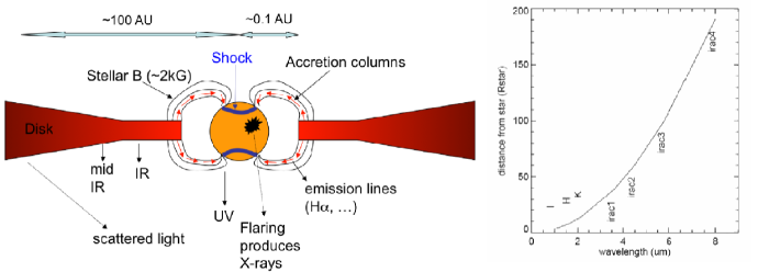
Figure 1.: LEFT: Anatomy of a young star, after Hartmann (1998). Not to scale! Note that the mid-infrared emission comes from relatively far out in the disk. RIGHT: Simplified version of relationship between peak emission wavelength and distance from the protostar. For a typical low-mass protostar, the near-infrared bands $I$, $H$, and $K$ sample within $\sim$10$R_{*}$; the four IRAC bands at 3.6, 4.5, 5.8, and 8 $\mu$m are sensitive to disk properties at $\sim$30–$\sim$200$R_{*}$.

2 MIR YSO variability in the pre-Spitzer era

Prior to the advent of the Spitzer Space Telescope (Werner et al. 2004), there were occasional published references to variability in YSOs in mid-infrared wavelengths, such as the following.

Prusti & Mitskevich (1994) originally set about looking for variations in all the repeated observations of Herbig AeBe (HAeBe) stars found at 12 and 25 $\mu$m in the Infrared Astronomy Satellite (IRAS) data taken in 1983. However, they found that source confusion was prohibitive, and focused their study on two HAeBe stars, AB Aur and WW Vul. They found significant variations on timescales ($t$) of months. They suggested that cometary clumps or a clumpy wind were plausible explanations for the variations observed.

Liu et al. (1996) reported that they found MIR variations in their ground-based data, ranging in amplitude from 30-300%, on timescales of days to years. They pointed out that the MIR variations most likely do not have the same origin as the optical/NIR variability. They suggest that since most of the MIR is from disk, then the cause of the variability must be there too. In order to achieve the variations that they observed, they postulate that the mass accretion rate ($\dot{M}$) varies by an order of magnitude. Small-amplitude changes in the MIR could be due to reprocessed accretion luminosity, whereas larger changes could be due to disk accretion rate, a disk instability, or outflow activity.

Abraham et al. (2004) took on the relatively difficult task of comparing Infrared Space Observatory (ISO) data taken in 1995-98 to MIR data taken at other bands with other facilities/instruments (such as MSX) at other epochs. They studied 7 FU Ori objects, and found weak MIR variability on timescales of years (over 1983–2001).

The next year, Barsony et al. (2005) reported on ground-based observations in the MIR of embedded objects in the $\rho$ Ophiuchi cloud core. By comparison to ISO data, they found significant variability in 18 out of 85 objects detected, on timescales of years. They found such variability in all spectral energy distribution (SED) classes with optically thick disks, and suggest that this might be due to time-variable accretion.

Later that year, in a large paper covering the MIR properties of the Orion Nebula, Robberto et al. (2005) reported on MIR variability in Orion, almost as an afterthought. They found variations up to $\sim$1 mag, on timescales of $\sim$2 years. They invoke changes in $\dot{M}$, activity in the circumstellar disk, or changes in the foreground $A_{v}$ to explain the variations they see.

Finally, Juhasz et al. (2007) report on the ISO variability of SV Cep. SV Cep is a UX Orionis-type variable, the generic properties of which include intermediate-mass YSOs with short ($t\sim$days-weeks) eclipse-like events in the optical. These could be edge-on self-shadowed disks, for example. This study is the only one (at least, the only one of which we have knowledge) reporting on a monitoring campaign conducted with ISO itself (as opposed to comparison of ISO data to data taken with other instruments/facilities). They obtained contemporaneous optical monitoring data over ISO’s lifetime (1995–1998) to aid in the interpretation of the MIR light curves. They found significant MIR variability on $t\sim$25 months; the MIR variations were anti-correlated with the optical variations but the far-IR variations were correlated with optical. They suggest a self-shadowed disk with a puffed-up inner rim, but find that this model does not do well at reproducing the MIR variations; again, $\dot{M}$ variations are invoked to explain the MIR variations.

3 Results in the Spitzer era

3.1 Introduction to Spitzer

The Spitzer Space Telescope (Werner et al. 2004) is an 85 cm, f/12 telescope. Before the on-board cryogen was exhausted, it operated at $<\sim$5.5 K, and was background-limited at 3-180 $\mu$m. It has two science cameras (Infrared Array Camera – IRAC – Fazio et al. 2004 and the Multiband Imaging Photometer for Spitzer – MIPS – Rieke et al. 2004), plus a low/moderate resolution spectrograph (Infrared Spectrograph – IRS – Houck et al. 2004). Launched August 2003 into an Earth-trailing orbit, it was 10-1000 times more sensitive than the 1983 IRAS mission.

The cryogen ran out in May 2009, and the telescope passively remains at $\sim$30 K. At this temperature, the IRAC 3.6 and 4.5 $\mu$m channels still operate essentially as they did before cryogen exhaustion, which is still 120-1000 times faster than VLT or Keck. This portion of the mission is “Spitzer-Warm”, and NASA has committed to fund $\sim$3 years of warm operations. As part of the Warm Mission, large ($>$500 hours), coherent observing programs were solicited, called “Exploration Science” programs.

The cryogenic Spitzer legacy for star formation research is substantial. There are multi-band maps of $\sim$300 square degrees of the Galactic plane, with $>$100 million sources. There are maps of $\sim$70 square degrees in nearby ($d<$500 pc) star-forming regions, with $\sim$8 million total sources in Taurus, Ophiuchus, Perseus, Chamaeleon, Serpens, Auriga, Cepheus, Lupus, Orion clouds, etc. Conservatively, we estimate that there are $\sim$20,000 YSOs in this rich data set.

Spitzer is a superb telescope for photometric monitoring because it is stable (better than 1%) and sensitive, wide-field (a single IRAC field of view is 5^′ on a side), Earth-trailing (so no orbital day/night aliasing), and it observes at bands sensitive to both photospheres and dust. In the Warm Mission era, we have the same amount of observing time as in the cryogenic era, and “just” 2 channels. There are several Exploration Science and smaller programs exploring the time domain with Spitzer.

3.2 Variability at Spitzer bands

YSO variability at Spitzer bands is unambigously apparent, and the torrent of papers on the subject is still ramping up. In the below, I discuss the papers in the order in which they appeared in the published literature.

The Legacy program “Cores to Disks” (c2d; Evans et al. 2003, 2009) took two epochs of observation (both IRAC and MIPS) separated by several hours to allow for asteroid removal. Several different papers (Alcala et al. 2008 and references therein) looked for variation between these two epochs (on timescales of $\sim$3-6 hrs), and did not find anything believable (within $\sim$25%) at wavelengths 3.6-24 $\mu$m.

Another Legacy program, “Surveying the Agents of a Galaxy’s Evolution” (SAGE; Meixner et al. 2006) studied the Large Magellanic Cloud (LMC), again in two epochs (both IRAC and MIPS), but this time separated by $\sim$3 months. Vijh et al. (2009) report on all of the variables found by comparing these two maps. They found mostly asymptotic giant branch (AGB) stars, which they point out is not entirely unexpected. However, we note here that optical variability is one of the defining characteristics of YSOs, and AGB stars are the most common “contaminant” in Spitzer selection of YSO candidates; having the right MIR colors plus MIR variability does not ensure that a given object is necessarily a YSO. Vijh et al. (2009) find 29 massive (=HAeBe) YSO candidates out of nearly 2000 variables, which they interpret to mean that at least 3% of all massive YSOs are variable. They also report that the amplitude of variability is often greatest at 24 $\mu$m, perhaps because most of their YSO SEDs peak at 24 $\mu$m (or longer).

The first high-cadence monitoring of young stars in IRAC bands was conducted by Morales-Calderón et al. (2009). The stars in IC 1396A were monitored twice a day for 14 d, plus every $\sim$12 s for 7 hrs. More than half of the YSOs showed variations, from $\sim$0.05 to $\sim$0.2 mag, on a wide variety of timescales, which enables the first possible serious physical interpretations of the variations. About 30% of the YSOs had quasi-periodic variations, on timescales of $\sim$5-12d periods, which they interpreted as 1 or 2 high-latitude spots illuminating inner wall of the circumstellar disk, plus a large inclination angle. Two objects have variations on timescales of $\sim$hours, but no color in the variations, which is interpreted as flares, and/or possibly $\dot{M}$ flickering. Other light curves are more likely due to varying $\dot{M}$ or disk shadowing. About 20% of the IC 1396A YSOs vary on $t\sim$days, without color changes, which could be due to $\dot{M}$ variations, and/or rapidly evolving spots. There are three objects that vary on timescales of days, with color variations, which the authors interpreted as radial differential heating of the inner disk, and possible inner disk obscurations. There were 46 variables not identified as YSOs (e.g., without a discernible IR excess); possibly they are YSOs or even AGBs, but more data are needed to interpret these. Larger amplitude variables tend to also be more embedded objects, but an order of magnitude change in $\dot{M}$ is needed to match the light curves, so this is probably not the dominant factor. A simple starspot is insufficient to explain the variability, but a hotspot combined with disk inhomogeneities does work. Also in the data was a young $\delta$ Scuti star, with a 3.5 hr periodicity on top of a $\sim$9 d period.

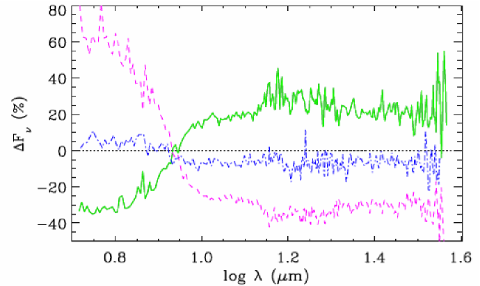
Figure 2.: Figure 1b from Muzerolle et al. (2009). Difference spectra between the first and second epochs (solid green), second and third epochs (dashed magenta), and third and fourth epochs (dash-dot blue), as a percentage change in flux. First epoch was 2007 Oct 9, second epoch was 2007 Oct 16, third epoch was 2008 Feb 24, and fourth epoch was 2008 Mar 2. Variations “pivot” at $\sim$ 8.5 $\mu$m, and are as large as 20-30% in a week.

Working in IC 348, Muzerolle et al. (2009) report specifically on the variations they observed in the T Tauri star LRLL 31. This object is identified specifically as a “transition disk”, meaning that it falls in a category of object thought to be in transition between a primordial, thick disk and a disk actively forming planets with gaps and structure in the disk created by protoplanets. The SED for this object suggests a large inner hole or gap. Muzerolle et al. (2009) initially noticed variations in IRAC+MIPS (3.6-24 $\mu$m) observations taken over $t\sim$5 months. They used both IRS and MIPS (5-40 $\mu$m) to further probe these variations on timescales of $\sim$days to $\sim$months. In the IRS spectra, reproduced in Figure 2, they found that the variations pivot at a point $\sim$8.5 $\mu$m, and they found variations of 20-30% within a week. They also found variations at 24 $\mu$m on $t\sim$1 day; recall Figure 1 – note that variations on those timescales are certainly not very far away from the star, even at that wavelength. Muzerolle et al. (2009) interpret these observations as vertical variations of an optically thick annulus located close to the star. Variations in $\dot{M}$ (up to a factor of 5) could be contributing here, or a companion causing gap, or even a warp.

Giannini et al. (2009) conducted observations of the Vela Molecular Ridge (VMR-D), with just IRAC. The two maps were taken $\sim$6 months apart. They simply accept variability of YSOs at the MIR bands as a defining characteristic of YSOs, as a statement of fact, and do not attempt to further justify it. This suggests a change in culture in the community. Giannini et al. (2009) conclude that 19 (out of $\sim$200) are likely variable young stars.

Bary et al. (2009) obtained IRS spectra of 11 actively accreting T Tauri stars in Taurus-Auriga; 2 of the 11 (DG Tau and XZ Tau) had significant variation in the 10 $\mu$m silicate feature on timescales pf $\sim$months to years (not weeks). They point out that this timescale is consistent with the source of the variations being motions of dust in the disk at $R<\sim$1 AU, and not with a clumpy dust envelope. Disk shadowing could still be possible, especially at the longer timescales. The possibility remains that there are binary companions to these objects as well. They had difficulty in fitting the line profile with existing models, suggesting that similar problems encountered by other investigators fitting single-epoch observations of other sources may ultimately be due to similar time-dependencies in those other sources. In any case, vertical mixing and disk winds are likely to be significant components of the source of the variability.

4 YSOVAR

John Stauffer leads the Exploration Science program (from Spitzer’s Cycle 6) entitled, “Young Stellar Object Variability: Mid Infrared Clues to Accretion Disk Physics and Protostar Rotational Evolution,” or YSOVAR. We were allocated 550 hours to conduct the first sensitive MIR (3.6 and 4.5 $\mu$m) time series photometric monitoring of several star-forming regions on timescales of $\sim$hours to years. Our fields include $\sim$1 square degree of Orion (centered on the Orion Nebula Cluster) plus smaller $\sim$25 square arcminute regions in 11 other well-known SFRs: AFGL 490, NGC 1333, Mon R2, NGC 2264, Serpens Main, Serpens South, GGD 12-15, L1688, IC1396A, Ceph C, and IRAS 20050+2070. Details of our fields, as well as a complete list of our collaborators, can be found at our website: http://ysovar.ipac.caltech.edu.

For our observations, we typically obtain $\sim$100 epochs/region (sampled $\sim$twice/day for 40d, less frequently at longer timescales). We started obtaining data in Sep. 2009 and will be obtaining data through June 2011. At the completion of our program, there should be good light curves for at least $\sim$2200 YSOs! We are also obtaining simultaneous (or nearly simultaneous) ground-based monitoring at $I_{c}$, $J$, and $K_{s}$, which aid significantly in our ability to interpret the light curves. (NB: if anyone in the community is interested in helping obtain such data, please contact us at ysovar-at-ipac.caltech.edu.)

Note that we include under the YSOVAR umbrella some affiliated programs such as J. Stauffer’s Cycle 7 Orion follow-up on some of our targets discussed below, P. Plavchan’s Cycle 6 Rho Oph intensive monitoring, K. Covey’s Chandra/Spitzer Ceph C monitoring, and J. Forbrich’s GGD 12-15 Chandra/Spitzer monitoring. As of this writing, there are five clusters with at least some data: Orion, L1688, Ceph C, IC 1396A, IRAS 20050.

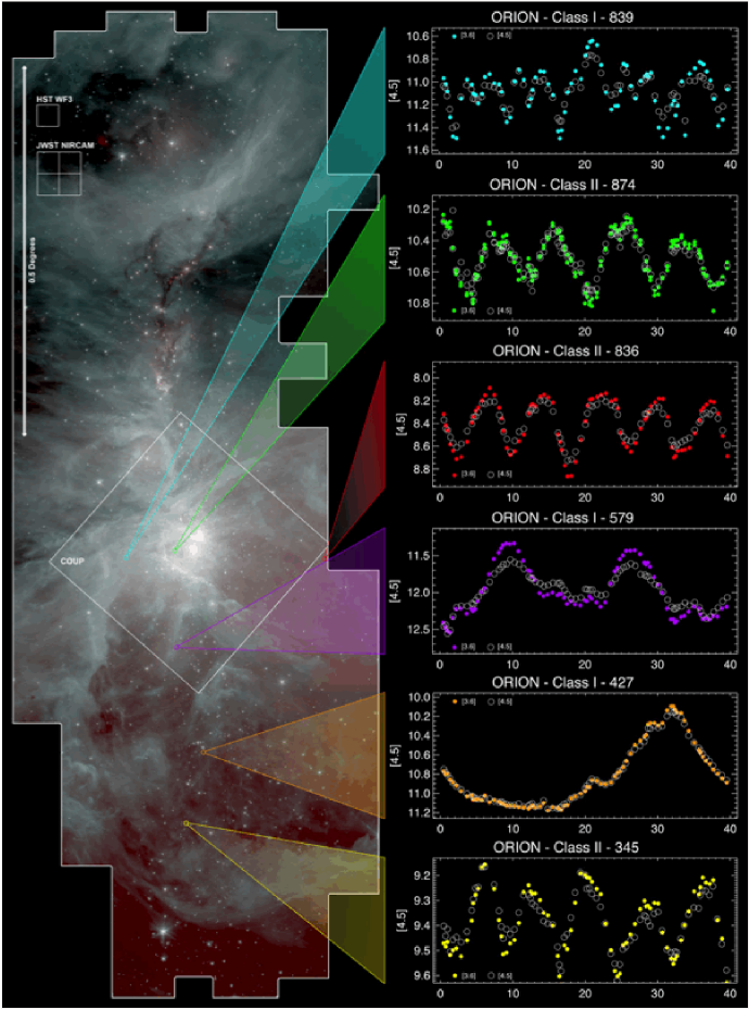
Figure 3.: Image depicting some of the variability found in YSOVAR observations in Orion. The image on the left is the two-band (3.6 and 4.5 $\mu$m) Spitzer composite. Indications of the relative sizes of 0.5^∘, and the Hubble WF3 and the JWST NIRCAM fields of view are in the upper left. The Chandra COUP field is indicated, centered on the Trapezium. For each of the light curves depicted, the solid point is 3.6 $\mu$m and the hollow point is 4.5 $\mu$m. Note the diversity of behavior exhibited by these variables.

Morales-Calderón et al. (2010, 2011; see also this volume) report on the early results from the YSOVAR monitoring of Orion. We find variability in $\sim$65% of the objects with infrared excess (Class I+II) and $\sim$30% of the objects without infrared excess (Class III). It should not be surprising that there is tremendously diverse behavior exhibited by these variables. Figure 3 shows just a sample of some of the light curves from some of the objects in Orion. The shape of the light curves likely have origins in slow changes in $\dot{M}$, changes in the $\dot{M}$ geometry, flares, photospheric spots, disk warps, and some causes yet to be identified! The contemporaneous optical and NIR data sometimes have a similar shape and amplitude as the MIR light curves, sometimes the NIR has a much larger amplitude, and sometimes the NIR variations are much smaller or not variable at all. In some cases, the NIR variations are phase-shifted with respect to the MIR. (See Morales-Calderón et al. 2010 for example light curves and more discussion.)

Because the emission in the MIR is likely coming from the disk (thermal dust emission) as well as the photosphere, the variations we see are likely due to variability in the disk as well as the photosphere. Thus, it is in general harder to derive a period for the central YSO for our target objects than from light curves, say, in $I_{c}$, where most of the emission comes from the photosphere (and spots rotating into and out of view generate rotationally modulated light curves). For just 16% of the variable objects with infrared excess (Class I+IIs) can we derive a period, and most of those are the ones with smaller excesses (90% of those are Class IIs, 10% are Class Is). For members without an IR excess, 40% are variables, and most of those are periodic. We can report $>$100 new periods. Of the Orion members with period measurements in the literature, we recover about 45% of those. There are also 10 eclipsing binaries, 5 of which are new discoveries (Morales-Calderón 2011).

One significant class of variables that we have discovered have AA Tau-like variations (see Bouvier et al. 2007 and references therein for discussion of AA Tau). These “dipper” stars have narrow flux dips, on timescales of days, and typically more than one dip are seen over our 40 d window; see Figure 4. In order for us to categorize a given object as a dipper, we require that the dip is seen in more than one epoch unless there are corroborating data at another band. Any optical or $J$ band corroborating data must have the dips be deeper by at least 50%. The “continuum” of the light curve must be flat enough that dip “stands out.” We find 38 Class I or II objects ($\sim$3%) in our set that are dippers, and we interpret this variability as structure in the disk, such as clouds or warps.

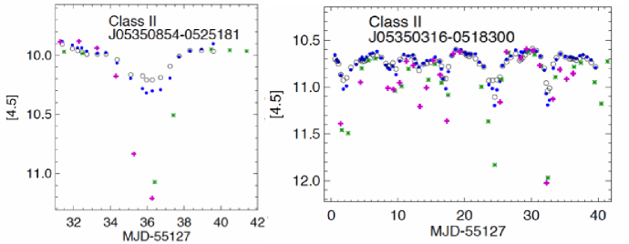
Figure 4.: Two examples of AA Tau-like (“dipper”) variability in our Orion data, from Morales-Calderón et al. (2010). Solid blue circles are 3.5 $\mu$m, open black circles are 4.5 $\mu$m, red or green $*$ are $J$, and magenta $+$ are $I_{c}$. The light curves are shifted in $y$-axis to align to the [4.5] “continuum” level.

Other upcoming results include the following. Plavchan et al. (priv. comm.) report that WL 4 is still eclipsing, 10 years after the 2MASS calibration data (Plavchan et al. 2008) were taken. This system is probably a quasi-stable disk eclipsing a binary system like KH-15D. Muzerolle, Flaherty et al. (priv. comm.; see also this volume) studied IC 348 and find IRAC variability (on timescales of days to years) in 56% of Class 0/I objects, 69% of Class II objects, and 58% of the transition disks. Moreover, even at 24 $\mu$m, 60% of Class 0/I, 40% of Class II, and 40% of transition disks vary! They also find dips in the light curves like the YSOVAR dippers.

The YSOVAR data set (as well as the associated programs) are certain to yield interesting results in the coming years. For lack of space, I have not addressed any possible monitoring results from Herschel or WISE, much less any recent non-MIR monitoring of young stars, such as CoRoT monitoring of NGC 2264 (see, e.g., Alencar et al. 2010 and references therein for more information).

5 Conclusions

While 15 years ago, we were as a community uncertain as to whether young stars vary in the mid-infrared, the literature suggested at least small variations on timescales of months to years, likely due to the disk. However, with the advent of the Spitzer Space Telescope and its stable, sensitive, wide-field platform for monitoring young stars, it has become unambiguous that yes, young stars vary in the mid-infrared, and they vary on pretty much any timescale that one cares to observe them (much as they do at many other bands). While definitive physical explanations for all of the tremendous diversity of variability types is still elusive, strong candidates for some types of variation are emerging. Some of the variability is clearly due to photospheric spots, much is due to structure in the disk, some is variation in mass accretion rate. Rotation, and the dynamic nature of the young star-disk system, are both clearly important. The answers are still forthcoming!

Acknowledgments

I wish to acknowledge many helpful conversations with J. Stauffer, M. Morales-Calderón, P. Plavchan, K. Covey, J. Carpenter, and the rest of the YSOVAR team. I also wish to thank J. Muzerolle for pre-publication access to his results. This work is based in part on observations made with the Spitzer Space Telescope, which is operated by the Jet Propulsion Laboratory, California Institute of Technology under a contract with NASA. Support for this work was provided by NASA through an award issued by JPL/Caltech.

References

- (1) Ábrahám, P., et al., 2004, A&A, 428, 89
- (2) Alcalá, J., et al., 2008, ApJ, 676, 427
- (3) Alencar, S., et al., 2010, A&A, 519, A88
- (4) Barsony, M., Ressler, M., & Marsh, K., 2005, ApJ, 630, 381
- (5) Bary, J., et al., 2009, ApJL, 706, 168
- (6) Bertout, C., 1989, ARA&A, 27, 351
- (7) Bouvier, J., et al., 2007, A&A, 463, 1017
- (8) Durán-Rojas, M. C., Watson, A., Stapelfeldt, K., & Hiriart, D., 2009, AJ, 137, 4330
- c2d (1) Evans, N. J., et al., 2003, PASP, 115, 965
- c2d (2) Evans, N. J., et al., 2009, ApJS, 181, 321
- (11) Fazio, G., et al., 2004, ApJS, 154, 10
- (12) Giannini, T., et al., 2009, ApJ, 704, 606
- (13) Hartmann, L., 1998, “Accretion processes in star formation”, Cambridge, UK ; New York : Cambridge University Press, 1998. (Cambridge astrophysics series ; 32) ISBN 0521435072.
- (14) Houck, J., et al., 2004, ApJS, 154, 18
- (15) Juhász, A., et al., 2007, MNRAS, 374, 1242
- Königl (1991) Königl, A. 1991, ApJL, 370, 39
- (17) Liu, M., et al., 1996, ApJ, 461, 334
- (18) Meixner, M., et al., 2006, AJ, 132, 2268
- mmc (1) Morales-Calderón, M., et al., 2009, ApJ, 702, 1507
- mmc (2) Morales-Calderón, M., et al., 2010, ApJL, submitted
- mmc (3) Morales-Calderón, M., et al., 2011, in preparation
- james (1) Muzerolle, J., et al., 2009, ApJL, 704, 15
- (23) Plavchan, P., et al., 2008, ApJK, 684, 37
- (24) Prusti, T., & Mitskevich, A., 1994, in The nature and evolutionary status of Herbig Ae/Be stars. Astronomical Society of the Pacific Conference Series, Vol. 62. Proceedings of the First International Meeting held in Amsterdam, 26-29 October 1993, San Francisco: Astronomical Society of the Pacific (ASP), edited by Pik Sin The, Mario R. Perez, and Edward P. J. Van den Heuvel, p.257
- (25) Rieke, G., et al., 2004, ApJS, 154, 25
- (26) Robberto, M., et al., 2005, AJ, 129, 1534
- Shu et al. (2000) Shu, F., et al. 2000, in Protostars and Planets IV, ed. V. Mannings, A. P. Boss & S. S. Russell (Tucson: University of Arizona Press), p. 789
- (28) Vijh, U., et al., 2009, AJ, 137, 3139
- (29) Watson, A., & Stapelfeldt, K., 2007, AJ, 133, 845
- (30) Werner, M., et al., 2004, ApJS, 154, 1