Toward Realistic Progenitors of Core-Collapse Supernovae

Abstract

Two-dimensional (2D) hydrodynamical simulations of progenitor evolution of a 23 $M_{\odot}$ star, close to core collapse (in $\sim 1$ hour in 1D), with simultaneously active C, Ne, O, and Si burning shells, are presented and contrasted to existing 1D models (which are forced to be quasi-static). Pronounced asymmetries, and strong dynamical interactions between shells are seen in 2D. Although instigated by turbulence, the dynamic behavior proceeds to sufficiently large amplitudes that it couples to the nuclear burning. Dramatic growth of low order modes is seen, as well as large deviations from spherical symmetry in the burning shells. The vigorous dynamics is more violent than that seen in earlier burning stages in the 3D simulations of a single cell in the oxygen burning shell (Meakin & Arnett, 2007b), or in 2D simulations not including an active Si shell. Linear perturbative analysis does not capture the chaotic behavior of turbulence (e.g., strange attractors such as that discovered by Lorenz (1963)), and therefore badly underestimates the vigor of the instability.

The limitations of 1D and 2D models are discussed in detail. The 2D models, although flawed geometrically, represent a more realistic treatment of the relevant dynamics than existing 1D models, and present a dramatically different view of the stages of evolution prior to collapse. Implications for interpretation of SN1987A, abundances in young supernova remnants, pre-collapse outbursts, progenitor structure, neutron star kicks, and fallback are outlined. While 2D simulations provide new qualitative insight, fully 3D simulations are needed for a quantitative understanding of this stage of stellar evolution. The necessary properties of such simulations are delineated.

1 Introduction

The first detailed calculations of the final, neutrino-cooled burning stages prior to core collapse of massive stars were done by Rakavy, Shaviv & Zinamon (1967), with simplified energy generation rates, and by Arnett (1968) using a small (24 species) network. Because of the extreme demands upon computer resources then available, simplified energy generation rates were used in subsequent calculations; see Arnett (1996) for references to the early work. This work showed two issues which have not yet be resolved: (1) the definition of convective zone boundaries involves incomplete physics (by construction mixing length theory ignores gradients, Spiegel (1971)), and (2) the stability of the burning in a convective region has not been demonstrated, only assumed. While thermal instability (thermal stability implies a global balance between nuclear heating and neutrino cooling in the convective zone) was considered (Arnett, 1972a, 1996)), dynamical instability (i.e., instability related to fluid flow) was not. In this paper we will show that both these issues are significant, and that they can be resolved by 3D numerical simulations and theory.

Almost all previous progenitor models for core collapse have focused on thermal behavior and quasi-static mixing, which are described by the evolution of the temperature and the composition variables. The dynamic behavior of the stellar plasma includes and is dominated by the velocity fields, which not only imply mixing, but also possible change in the stellar structure. The star is not necessarily a quasi-static object, but may have significant fluctuations in its variables. The dynamical behavior, found here for simultaneous, multi-shell burning, will drive entrainment (Meakin & Arnett, 2007b) at convective shell boundaries, changing the nucleosynthesis yields and the size of the Fe core at collapse.

The presupernova structure of a massive star consists of a core, mantle, and envelope. The envelope is extended, composed of H and He, and may have been removed prior to core collapse by wind-driven mass loss, or tidal stripping by a companion. The mantle is composed of burning shells of C, Ne, O and Si; these shells are convective, interact nonlinearly, contain most of the nucleosynthesis products ejected, and may smother a neutrino-driven explosion. The core is composed of Fe-peak nuclei, and its mass is determined by its entropy and electron fraction. Lower entropy and electron fraction give smaller cores, which are easier to explode by neutrino transport mechanisms. Core collapse mechanisms for explosion are sensitive to core mass, mantle density, and rotation; all are sensitive to the treatment of turbulence. The simulations described here involve the simultaneous action of C, Ne, O and Si burning shells. The oxygen shell is special, because (1) formation of electron-positron pairs softens the equation of state, aiding the formation of large amplitude motion, (2) the large abundance of oxygen and its relatively large energy release per unit mass provide a large thermonuclear energy reservoir, and (3) oxygen burning, unlike silicon burning, has little negative feedback from quasi-equilibrium to damp flashes (see below).

In Section 2 we discuss the historical context of progenitor models of core collapse supernovae, focusing on issues of mixing, causes of time-dependence and multi-dimensionality, prospects for development of better computational tools, and the differences between 2D and 3D simulations. In Section 3 we describe our 2D simulations of progenitor evolution with multiple, simultaneously active, burning shells (C, Ne, O, Si), and discuss some new phenomena which appear. In Section 4 we summarize the implications for evolution prior to core collapse. In Section 5 we focus on several problems in observational astrophysics which need to be reconsidered in light of our results. In Section 6 we summarize the major conclusions, and outline the necessary features of new 3D simulations which will be required to quantitatively resolve the issues presented by the 2D simulations.

2 Brief Historical review of 1D, 2D, and 3D Models

2.1 1D Models: Mixing

By the term advection we mean the transport of a parcel of matter by a large-scale flow; by diffusion we mean the transport of a parcel of matter by a random walk of small-scale motions (often microscopic motion of ions in the stellar plasma). The mass (baryon) flux due to advection is

$${\bf F_{m}}={\bf u}\rho,$$ (1)

where $\bf u$ is the fluid velocity vector and $\rho$ is the mass (baryon) density. The flux of any scalar variable is related to this flux by a factor of the density of the variable per unit mass (baryon). For example, if the mass (baryon) fraction of nuclear species $i$ is $X_{i}$, the flux of this species is

$${\bf F_{i}}={\bf u}\rho X_{i}={\bf F_{m}}X_{i}.$$ (2)

The rate of change due to such fluxes involves a divergence, as in the continuity equation,

$$\partial\rho/\partial t=-{\bf\nabla\cdot F_{m}}.$$ (3)

Thus, 1D advection involves a first order spatial differential operator.

If the considered volume contains heterogeneous (turbulent) matter, the flux may vary over the corresponding surface. If that volume is a zone in a stellar evolution computation, then the fluxes must be averaged over the heterogeneity, and some knowledge (or assumption) regarding the smaller scale structure is required. Consider the simple example of only an inflow and an outflow, and variation only in the vertical direction. The net flux for species $X_{i}$ is then

$$F_{net}(X_{i})=-(F_{m}X_{i})_{out}+(F_{m}X_{i})_{in}.$$ (4)

Suppose that $F_{out}=F_{in}\equiv\rho u$, so $F_{out}-F_{in}=0$, which automatically satisfies mass (baryon) conservation, so that

$$F_{net}(X_{i})=-\rho u\Big{[}(X_{i})_{out}-(X_{i})_{in}\Big{]}.$$ (5)

In this case the flux (of composition $i$) is proportional to the negative of the difference in abundance in the up and down flows.

For diffusion, the number flux follows from Fick’s law,

$${\bf\mathcal{F}_{d}}(X_{i})=-{1\over 3}\lambda v{\bf\nabla}N_{i},$$ (6)

and is proportional to the gradient of a number density $N_{i}$. Here $\lambda$ is a mean-free-path and $v$ is a speed of diffusing particles. The number density for species $i$ may be written as $N_{i}=\rho{\cal A}X_{i}/A_{i}$, where ${\cal A}=1/m_{amu}$ is Avogadro’s number (the inverse of the atomic mass unit) and $A_{i}$ is the number of nucleons in species $i$. The mass (baryon) flux is ${\bf F_{d}}(X_{i})=A_{i}m_{amu}{\bf\mathcal{F}_{d}}(X_{i})$. Thus,

$${\bf F_{d}}(X_{i})=-{1\over 3}\lambda v{\bf\nabla}(\rho X_{i}).$$ (7)

If we consider the divergence of the flux, diffusion implies a second order spatial differential operator, in contrast to advection which, as we saw, implies first order. This is a fundamental mathematical difference.

Weaver, Zimmerman & Woosley (1978); Woosley, Heger, & Weaver (2002) introduce an effective diffusion coefficient $D$ to model convection:

$${dY_{i}\over dt}={\partial\over\partial m}\Big{[}(4\pi r^{2})^{2}\rho^{2}D{\partial Y_{i}\over\partial m}\Big{]}.$$ (8)

In the case of a region unstable to convection by the Ledoux criterion, they take $D_{c}\equiv v_{c}\ell/3$, where $v_{c}$ is the velocity estimated by mixing-length theory (Böhm-Vitense, 1958; Clayton, 1983) and $\ell$ is the mixing length. Thus if

$$\lambda v=\ell v_{c},$$ (9)

then Equation  7 is recovered. The use of Equation 7 requires that $\lambda\ll\Delta r$, where $\Delta r$ is a zone size. For a turbulent cascade, $\ell\gg\Delta r$, which is inconsistent with the previous requirement. The treatment of convection as diffusion is essentially an algorithmic interpolation procedure, but has an intrinsic contradiction in physics. This arises because turbulent flow has two facets: a flow at large scale $\ell$ which does most of the transport, and a flow at small scale $\lambda$ which does the dissipation, and $\ell\gg\lambda$. The diffusion approximation might be used for the small scale flow, but that is irrelevant to the transport problem, which is dominated by the large scale flow (Arnett, Meakin, & Young, 2009).

Notice the rough similarity between Equation 5, which represents the underlying fluid dynamics (Landau & Lifshitz, 1959), and Equation 7, which represents the proposed approximation. Taking the density outside the differential operator and using a finite difference representation of Equation 7,

$${\bf F_{d}(X_{i})}\sim-\Big{[}{1\over 3}\lambda v\rho/\Delta r\Big{]}\Big{[}(X_{i})_{out}-(X_{i})_{in}\Big{]}.$$ (10)

For this to be consistent with 1D advection (Equation 5) we must have a diffusion rate that is dependent upon the zoning! While perhaps useful algorithmically, this is not clear conceptually; see also the discussion of Maeder & Meynet (2000), who also express doubts concerning the approximation of advection by diffusion.

Mathematically, diffusion is a procedure which maximally smooths gradients, so that a more realistic procedure may be expected to exhibit less smoothing. While based on poor physics, the diffusion model of convection had the virtue that it allowed numerical prediction of yields.

Much effort has recently gone into extending stellar evolution to include rotational effects (Zahn, 1992; Chaboyer, Demarque, & Pinsonneault, 1995; Maeder & Meynet, 2000; Tassoul, 2000; Woosley, Heger, & Weaver, 2002). Evolution of a rotating star will develop differential rotation in general, and shear flow. Similarly, deceleration of convective plumes will develop shear flow. In stars both flows will be turbulent. Convection and rotation have an underlying similarity not reflected in stellar evolution theory. The review of Maeder & Meynet (2000) gives a clear presentation of the various approximations involved in reducing the full fluid dynamic equations to a simpler, more easily solvable set. It is now possible to test these approximations by numerical simulation in both shearing box (Arnett & Meakin, 2009; Stone & Gardiner, 2010) and whole star domains (Brun & Palacios, 2009; Brown, et al., 2010); see also the theoretical developments of Balbus (2009); Balbus & Weiss (2010). A theoretically sound approach must treat the shear from differential rotation and the shear from convective plumes on a consistent basis, reflecting their underlying physical similarity (Turner, 1973).

2.2 Time Variation

The $\epsilon$-mechanism. The $\epsilon$-mechanism (Ledoux, 1941, 1958) for driving stellar pulsations by nuclear burning was examined by Arnett (1977) for Si burning in 1D geometry, using the simple energy generation rate proposed by Bodansky, Clayton & Fowler (1968). In this case, explicit 1D hydrodynamic simulations gave nuclear-energized pulsations (see Figure 6 in Arnett (1977)). There were two high frequency modes (period  $0.1$ seconds and $1$ second) and a lower frequency convective mode (turnover time $\sim 20$ seconds). The intermediate frequency mode was related to the Si flash. Computation with a realistic nuclear network subsequently showed that the highest frequency (“acoustic”) pulsations would be strongly damped due to the quasi-equilibrium nature of Si burning; an increase in temperature gave an increase in free alpha particles (and neutrons and protons), which required energy, and resisted the increase in temperature (with an almost 180 degree phase shift, meaning that there is strong negative feedback to resist changes). However, this damping process does not apply to O, Ne or C burning, which have little or no quasi-equilibrium behavior, and in principle could drive pulsations more vigorously.

The $\tau$-mechanism. Arnett & Meakin (2011b), in study of the 3D simulations of Meakin & Arnett (2007b), found that the bursts in turbulent kinetic energy were related to similar fluctuations in the Lorenz (1963) model of a convective roll; this is the now-famous strange attractor. This instability mechanism, called the $\tau$-mechanism for “turbulence”, is expected to be a general property of stellar convection zones, and probably is the cause of the fluctuations in luminosity observed in irregular variables (e.g., Betelgeuse, see Arnett & Meakin (2011a, b)). This process is independent of the temperature and density dependence of the thermonuclear heating, and thus is distinctly different from the $\epsilon$-mechanism. Unlike the $\epsilon$-mechanism, the $\tau$-mechanism is not a linear instability, but is inherently nonlinear.

In appropriate circumstances however, the $\tau$-mechanism may couple to nuclear burning, making pulsations more violent, giving a more complex, combined $\epsilon+\tau$ mechanism. The $\tau$ mechanism involves a non-linear instability, unlike the linear instabilities discussed by Goldreich, Lai & Sahrling (1997). In a detailed analysis, Murphy, Burrows & Heger (2004) solve the linear perturbation equations for several massive stars prior to core collapse, and based upon the $\epsilon$ mechanism alone, find inadequate driving to cause such violent behavior as is actually shown in the non-linear simulations presented below.

The analysis of Murphy, Burrows & Heger (2004) is perfectly correct within framework of the linear assumption, but the assumption fails. The linear approximation is not valid in this case because turbulence is not a linear perturbation of the system. Lorenz (1963) showed that chaotic behavior in a convective roll is due to the nonlinear interaction between temperature gradients (both vertical and horizontal) and convective speed. Solutions which are initially close to each other will diverge exponentially as time passes. Thus the interplay between pulsation and turbulent convection is not captured by traditional linear perturbation analysis of stellar pulsations. This is an interesting theoretical result, suggesting that linear perturbative methods for pulsations (Cox, 1980; Unno, et al., 1989) may require reexamination when turbulent convection is important (as those authors feared).

2.3 History of Multi-dimensional Progenitor Models

There have been relatively few multi-dimensional simulations of core collapse progenitors, but there has been a rich context of efforts on turbulence and stellar hydrodynamics (Porter & Woodward, 1994, 2000; Fryxell, Müller, & Arnett, 1989), on the helium flash (Deupree, 1984, 1996, 2003; Dearborn, Lattanzio, & Eggleton, 2006; Moćak, et al., 2008, 2009, 2010), and on turbulent MHD with rotation (e.g., m-dwarf simulations by Browning (2008)), as well as extensive work on the Sun with the ASH code (e.g., Brown, et al. (2010)) and on stellar atmospheres pioneered by Nordlund and Stein (e.g., Nordlund, Stein, & Asplund (2009)). This context has speeded the development of tools and helped determine their reliability. The first effort at simulating oxygen burning (Arnett, 1994) helped define the shell burning problem with regard to required resolution, but suffered from the use of sectors so narrow in angle that boundary effects affected the flow.

Table 1: Two-dimensional Progenitor Simulations

Reference	$a$	$b$	$c$	$d$	$e$
zoning	256x64	256x64	172x60	800x320	800x320
code	PROMETHEUS	PROMETHEUS	VULCAN	PROMPI	PROMPI
eosf	wda	wda	wda	TS	TS
network	12	123	12	25	37
burning	O	Si	O	C,Ne,O	C,Ne,O,Si
core	Si	Si	Si	Si	Fe
duration(s)	300	200	1200	2500	600

Table 1 summarizes aspects of early 2D simulations of progenitor models in comparison to the present work. The first 2D hydrodynamic simulations of core-collapse progenitors (oxygen burning) showed striking new phenomena: mixing beyond formally stable boundaries, hot spots of burning due to $\rm C^{12}$ entrainment, and inhomogeneity in neutron excess (Bazàn & Arnett, 1994). Further work (Bazàn & Arnett, 1998) confirmed that convection was too dynamic to be well represented by diffusion-like algorithms, that large density perturbations (8%) formed at convective boundaries, and that gravity waves were vigorously generated by the flow. Extension to Si burning (Bazàn & Arnett, 1997b) with a 123 isotope network showed similar highly dynamic behavior and significant inhomogeneity in neutron excess. With an entirely different 2D code (VULCAN), Asida & Arnett (2000) extended the evolution of the oxygen shell of Bazàn & Arnett (1998) to later times, and discovered that the extensive wave generation at the convective boundaries induced a slow mixing in the bounding non-convective regions.

Kuhlen, Woosley, & Glatzmaier (2003) investigated shell oxygen burning in 3D with an anelastic hydrodynamics code (Glatzmaier, 1984), and found small density and pressure perturbations (less than 1%). The boundary conditions were impermeable and stress-free, so that convective overshoot could not be studied. They concluded that, contrary to previous work listed above (done with 2D compressible codes), the behavior was not very dynamic and could be described by the MLT algorithms used in 1D stellar evolution codes (e.g., Weaver, Zimmerman & Woosley (1978)). Meakin & Arnett (2007a), using 3D compressible hydrodynamics, showed that the differences were due to the choice of (unrealistic) boundary conditions that Kuhlen, Woosley, & Glatzmaier (2003) used. Inside the convection zone, away from the boundaries, the Glatzmaier code gave results in good agreement with the compressible code. However, as stressed in Bazàn & Arnett (1998), fluid boundaries allow surface waves to build to large amplitudes ($\delta\rho/\rho\sim 0.1$), so that the hard boundaries used in Kuhlen, Woosley, & Glatzmaier (2003) distorted the physics. The good agreement between the anelastic and the compressible solution within the convection zone, and the agreement between the stable layer dynamics given by the compressible fluid code and analytic solutions to the non-radial wave equation, indicate that the compressible hydrodynamic techniques are robust for this problem, even for Mach numbers below 0.01. An anelastic code with the correct boundary conditions should give the same result; the flow is subsonic.

With the PROMPI code (Meakin, 2006), several new series of computations were done. Meakin & Arnett (2007a, b) presented the first 3D calculations of the phase of shell O burning with full physics (i.e., compressibility, nuclear network, real equation of state, appropriate boundaries, etc.). Meakin & Arnett (2006) calculated in 2D the oxygen burning shell, and both C and Ne burning shells above this. Here we present simulations (Meakin, 2006) with similar microphysics, extended to include the silicon burning shell as well, so that C, Ne, O and Si burning occur on the grid, but only in 2D.

2.4 Future Prospects: Beyond 2D

Progress will not be a simple progression reflecting the growth of computational resources, but also of theoretical understanding. Arnett & Meakin (2011b) have shown a connection between the Lorenz model of a convective roll and the bursty pulses in turbulent kinetic energy seen originally in the Meakin & Arnett (2007b) simulations, which seem to have a similar strange attractor. The Lorenz model is a low order (3 variable) dynamical system, and its physical identification with the 3D simulations suggests how we may project the essence of the 3D solutions onto 1D for stellar evolution and dynamics (“321D”). This will give an immediate improvement over MLT as well as better initial models for numerical simulation; see below. The physical basis is strengthened mathematically by use of the Karhunen-Loève or proper orthogonal decomposition (POD; see Holmes, Lumley, & Berkooz (1996)) of the 3D numerical data set of Meakin & Arnett (2007b). Preliminary results show that roughly half of the turbulent kinetic energy is in the single lowest order empirical eigenmode, supporting the idea that low order dynamical systems may be used to describe the complexities of time dependent turbulent flow in stellar convection zones.

The dynamical phases prior to core collapse may not attain a statistically averaged state, so that these methods (321D and KL decomposition), while promising for earlier evolution, may not be the optimum tools for the pre-collapse itself, where large eddy simulations (ILES, Boris (2007)) in 3D are needed. However, use of the theoretical tools (321D and KL decomposition) provides a means of estimating the range of fluctuations about an given ILES simulation, which may be tested insofar as computational resources allow, for other initial conditions.

2.5 Comparison of 2D and 3D Simulations

Meakin & Arnett (2007b) show a precise comparison of two simulations, which use the same microphysics, initial model and code, and differ only in dimensionality, which changes from 2D to 3D. The simulations are discussed there as “core convection” (see Figure 4 therein). The topology of the convective flow is significantly different between 2D and 3D models: the 3D convective flow is dominated by small plumes and eddies while the 2D flow is much more laminar, and dominated by large vortices (“cyclones”) which span the depth of the layer. The 2D vortices trap material which is slow to mix with surrounding matter; in 3D the flows become unstable and matter mixes more completely. The wave motions in the stable layers do not have an identical morphology in 2D and 3D, and the velocity amplitudes are much larger in 2D.

The differing behavior is due to the constraint of geometry, and the law of angular momentum conservation, which forces the formation of large cyclonic patterns in 2D that are unstable in 3D. The turbulent cascade moves from small scale to large (cyclones) in 2D, but from large to small (Kolmogorov cascade) in 3D. Cyclonic behavior at large scales is physically reasonable for the Earth’s atmosphere, for example, which because of its restriction in height, is approximately two-dimensional. In stars there is no physical constraint to enforce 2D motion, so that 2D simulations of stars are not realistic, merely computationally less expensive.

In Meakin & Arnett (2007b), 3D simulations were done for a single cell in the O shell; the computational demands for simultaneous multi-shell burning are more extreme (but almost feasible). As a first step we present 2D simulations, which though flawed, are instructive. We describe the first extended results for four simultaneous burning shells (Si burning included, Meakin (2006)), and interpret them with the benefit of extensive analysis of 3D O burning results. Taken with Figure 4 from Meakin & Arnett (2007b), they provide clues about the nature of the true behavior to be expected in 3D.

3 2D Simulations of Multiple Simultaneously Burning Shells

3.1 Starting Point

The initial conditions are a fundamental problem for numerical simulations which explore the development of instabilities to large amplitude. Subtle biases in the initial state might make the subsequent development misleading. Use of a 1D initial model, with no reliable description of the turbulent velocity field or the extent and position of the boundaries of the convection, is a cause for worry, but is the best we can do at present.

The 2D simulations started from a model obtained from a sequence by P. A. Young (private communication; Fryer, Young, et al. (2008) have evolved this model to core collapse in 1D, and to 3D explosions). The initial state was a 1D model of a 23 $M_{\odot}$ star, mapped to 2D; it is at the latest stages of evolution, about one hour prior to core collapse. Turbulent convection developed from very small perturbations ($\sim 10^{-3}$ or less, due to mapping onto a different grid) in the unstable regions. The convection rapidly evolved to a dynamic state with far larger fluctuations, independent of the initial perturbations. The model was similar to that used in Meakin & Arnett (2007b), except the computational volume is deeper, reaching down past the Si burning shell, the aspect ratio is larger (a full quadrant was calculated), the abundance gradients were smoother (more like a diffusion approximation for convection; see § 2.1), and the onset of core collapse was much nearer ($\sim 1$ hour).

Figure 1: Thermonuclear reaction network (37 nuclei) used for burning in C, Ne, O, and Si shells. Each box represents a nucleus; see text for details.

The computational domain had an inner boundary representing the Fe core and extended well beyond the active burning regions to the edge of the He core. The boundary conditions in angle were periodic and in radius were reflecting, as in Meakin & Arnett (2006, 2007a, 2007b). The equation of state was that of Timmes & Swesty (2000), which accurately describes the effects of partial relativistic degeneracy of electrons and of the formation of electron-positron pairs, and is very similar (Timmes & Arnett, 1999) to the equation of state used in previous simulations listed above.

Figure 1 shows the nuclear reaction network used, which contained 38 species (37 isotopes plus electrons). To deal with increasing neutron excess it was extended to $\rm Ni^{62}$, which corresponds to ${\rm Z/A}\sim 0.45$. During Si burning, the nuclei having $\rm Z\geq 22$ approach a local nuclear statistical equilibrium (they become a quasi-equilibrium group). The results of this network were compared to those of a 177 isotope network; it reproduced both the energy generation and the increase in neutron excess predicted by the larger network (see discussion of nucleosynthesis and of increase in neutron excess during silicon burning in Arnett (1996)). The nuclear burning was directly coupled to the fluid flow by the method of operator splitting.

3.2 Results

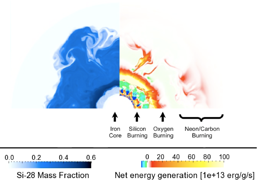
Figure 2: A snapshot of the structure of C, Ne, O, and Si shells surrounding the Fe-core of a pre-collapse progenitor of 23 $M_{\odot}$  star, about 500 seconds after the constraint of spherical symmetry has been removed. The left side shows the abundance of $\rm Si^{28}$ while the right side shows the net energy generation rate.

Figure 2 shows the structure of a quadrant of the core of the $23$$\,M_{\odot}\/$ star, with an iron core (shown as a white semi-circle) in the center. The computational domain includes burning shells of Si, O, Ne and C, in order of increasing radius. The left quadrant displays abundance contours of $\rm Si^{28}$ (dark blue is high abundance, white is low). The inner light region is a burning shell which is depleting its Si. Above this is a dark ring which is unburned Si. Further out is a medium blue layer which contains the O burning shell, in which Si is being produced. At the top of this layer are seen streams of very light blue, denoting entrainment of matter which has not been contaminated by oxygen burning (mostly C and Ne). Finally there is a very light blue layer from which the streams came, and which has no enhancement of Si above its original value.

The right quadrant shows contours of energy generation rate, in units of $10^{13}$ erg/s. Note that the second quadrant is presented as a rotation about the vertical axis; this helps identify corresponding matter in the two different variables which are mirror images. The inner ring is again the Si burning shell. It has both strong heating (yellow) and strong cooling (blue) at the same radius, that is, the burning does not possess spherical symmetry. This is enclosed by a green ring, the Si rich layer, which has milder neutrino cooling, and is no longer spherically symmetric because of “hot spots” of burning in entrained (descending) plumes. Beyond this is a ring of red and yellow which is highly dynamic: the O burning shell itself. Finally, above this wisps and plumes of heating are beginning to be seen; these are due to C and Ne burning in entrained matter which is rich in these fuels.

These models have a low Damköhler number (Damköhler, 1940), $D_{a}=\tau_{turbulence}/\tau_{react}\ll 1$, where the time scale for turbulent flow is $\tau_{turbulence}$ and the reaction time is $\tau_{react}$. In this limit a complex mixing model is not needed to describe the burning, unlike burning fronts in type Ia supernova models which require a more complicated description. Here fuel is transported into regions of higher pressure, compresses and heats, burns, expands and cools, and is buoyantly transported back to lower pressure. Changes in composition due to turbulent mixing are much faster than those due to nuclear burning, so that a sub-grid flame model is not required.

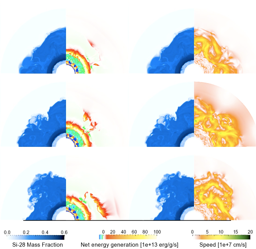
Figure 3: Snapshots of the structure of C, Ne, O, and Si shells surrounding the Fe-core of a pre-collapse progenitor of 23 $M_{\odot}$  star. Three different times are shown, $t_{f}$ = 0, 61, 83 seconds (from top, 0 s, to bottom, 83 s) after our fiducial model (see text). The left panels (blue) show abundance of $\rm Si^{28}$, while the right panels show energy generation rate and convective speed, respectively.

The initial model was strictly spherically symmetric, and had to develop a self-consistent turbulent velocity field to carry the heat from nuclear burning away from the burning regions. During this mild transient phase, asymmetries begin to develop slowly. Figure 2 shows the structure after this development, and at the beginning of significant deviation from the usually assumed spherical symmetry. Because of the time needed for the initial spherical model to develop a realistic and consistent convective flux, there is ambiguity regarding the “initial time”; we simply define a “fiducial time” ($t_{f}=t-t_{0}$ where $t_{0}\sim 345$ seconds into the 2D simulations) at which the model is still fairly spherical but has a realistic convective flux, and we count elapsed time after that.

Figure 3 shows three snapshots of the structure at different times after the fiducial time: $t_{f}$ = 0, 61, and 83 seconds. The left column represents the same variables as shown in Figure 1. The right column shows the $\rm Si^{28}$ abundance as before in the left panel, but in the right panel the energy generation rate is replaced by the turbulent speed in units of $10^{7}$ cm/s.

Distortions in the O burning shell are obvious. The equation of state in this region is affected strongly by the thermal production of an equilibrium abundance of electron-positron pairs, so that the effective adiabatic exponent drops below $\Gamma_{1}\sim 4/3$. Similarly $\Gamma_{4}\equiv 1+E/PV\sim 4/3$; This means the local contribution to the gravitational binding energy, which is proportional to $\Gamma_{4}-4/3$, is small. This is a common property of oxygen burning in stars Arnett (1968, 1996). The restoring force for stable stratification is weak, allowing large amplitude distortions with little energy cost.

The decrease in $\Gamma_{1}$ and $\Gamma_{4}$ are due to the need to provide the rest mass for newly formed electron-positron pairs. At low temperature, $kT\ll 2m_{e}c^{2}$, the number density of pairs relative to the charge density of ions decreases exponentially with decreasing temperature, and is negligible. As temperature approaches $T\sim 2\times 10^{9}$ degrees Kelvin, the effect on the equation of state becomes largest. At higher temperatures, the increase in mass of pairs is less relative to the thermal energy $kT$, so that these gammas approach that of an extreme relativistic gas, $\Gamma_{1}=\Gamma_{4}=4/3$. Oxygen burning ($\rm O^{16}$ fusion) in stars occurs at $T\sim 2\times 10^{9}$ degrees Kelvin, so that this burning stage is most influenced by the effects of electron-positron pair production on the equation of state.

Consider first the left column in Figure 3. The top panel (t=0) is relatively symmetric, but as time passes, the middle and lower panel show increasing distortion, especially visible at the interface between the outer, light blue layer and the middle, medium blue layer. The streams of light blue inside the medium blue represents entrainment of matter with little Si, that is, C and Ne fuel. This corresponds to the flame structures seen in the right side of the left column, which are due to C and Ne burning (note similarity in shapes on left and right sides in the left column). Similar entrainment is occurring at the top of the Si burning convective region; the outer edge of the light blue inner ring is rippled due to bursts of burning. The amplitude of these variations is smaller due to the stiffer equation of state here.

The right side of the right column shows the turbulent convective speed. The large structures are the oxygen burning convective zone. A smaller convection zone may be seen surrounding the Fe core, due to the Si burning shell. The C-Ne layer, lying outside the oxygen burning shell, illustrated the effect of a low-order mode. In the top and bottom panels, there is little motion, while in the middle panel the amplitude of the motion is near maximum. The lighter red areas at about 30 degrees and 70 degrees from vertical correspond to nodes in the modal velocity. Because of symmetry about the equator (horizontal) we have four nodes in 180 degrees, or an $\ell=4$ mode being dominant. Odd values of $\ell$ are suppressed by the domain size and symmetry imposed by our boundary condition, so this is the lowest order possible in this simulation; it has a period of about 60 seconds, but is mixed with other, weaker modes. A movie of the simulation shows a dramatic change as this mode turns the speed on and off as we move from top to middle to bottom.

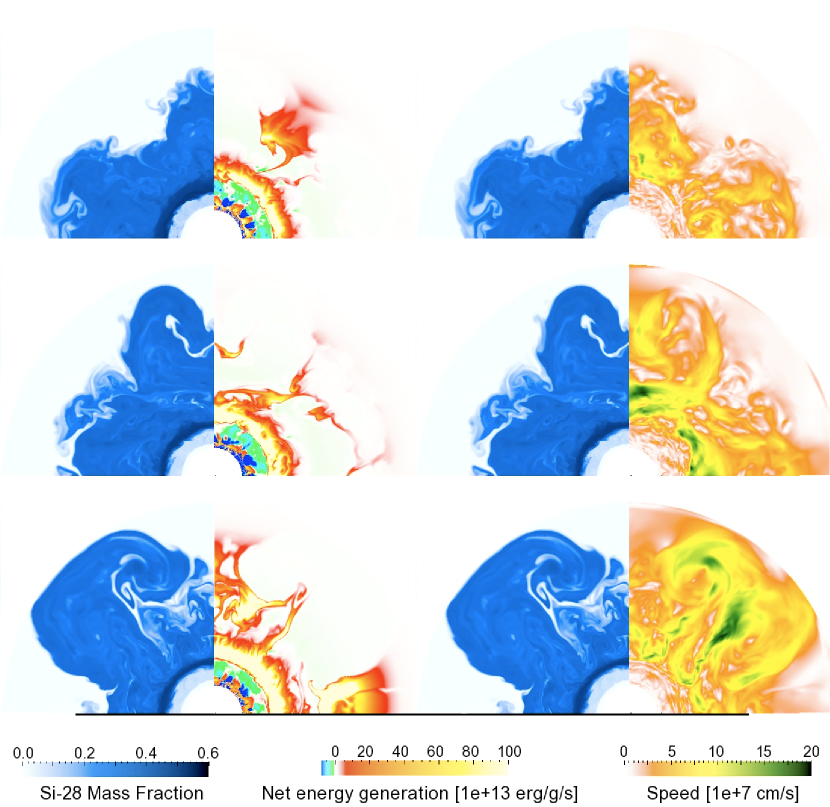
Figure 4: Structure of C, Ne, O, and Si shells surrounding the Fe-core of a pre-collapse progenitor of 23 $M_{\odot}$  star. Snapshots at times $t_{f}$ = 115, 247, and 307 seconds (top to bottom) after our fiducial model (see text). The format is the same as in Figure 3. The eruption has become strongly non-linear, as the bottom panels show.

Figure 4 shows the same variables at t = 115, 247, and 307 seconds, after several, increasingly vigorous “sloshes”. The distortion in the O shell has grown, with large amplitude motions whose wave-form is characteristic of $g$-modes. Entrainment of C and Ne increases. Fluctuations in Si burning become more vigorous and distort the Si layer although quasi-equilibrium damps explosive excursions. The Si shell burning occurs in dynamically forming and disrupting cells, qualitatively similar in nature to the 3D cell studied in Arnett & Meakin (2011b). A pink tinge indicates weak but widespread burning of carbon in the outer layers of the computational domain.

At $t_{f}=307$ seconds what is best described as an “eruption” is occurring. The distortion in the O shell (medium blue bulge) continues to grow; it is due to strong wave motion, powered by the nuclear burning. In the bottom panel, the thickness of the O shell convective layer varies by more than a factor of three as a function of angle; it is thin at the equator and thick at a 45 degree angle. This corresponds to an eruption at that angle. Entrainment is correspondingly increased, with consequent burning. Waves ”slosh” back and forth. The computational domain and boundary conditions restrict the lowest order modes. The Si burning shell is affected by the behavior of the O shell. There appears to be no evidence of a slacking in growth of the dynamic behavior, and extensive mixing is occurring. We ended the simulation because the extent of mixing is so great that it reaches the grid boundaries, and the simulation domain becomes inadequate. The assumption of spherically symmetric structure has clearly failed, as has the assumption of quasi-hydrostatic structure.

4 Implications

Figures 3-4 show the breakdown of the assumption of spherical symmetry, which has been the basis of supernova progenitor models, and much of the interpretation of observational data of supernovae and young supernova remnants. The $\ell=4$ spherical harmonic is dominant because the computational domain had only one quadrant and periodic boundaries; a full hemisphere would have allowed the $\ell=1$ mode to appear.

These simulations, of a stage only one hour before core collapse, show more violent behavior than previous 2D simulations of multiple (CNeO) shells (Meakin & Arnett, 2006), or 3D simulations with a single burning shell (Meakin & Arnett, 2007b). They become more violent in less time; compare durations in Table 1. There are several reasons for this behavior. (1) This stage is late, only an hour prior to collapse. (2) The 3D O shell simulations had a smaller computational domain, so that low order modes were restricted by periodic boundary conditions. (3) The difference between the 2D three shell (CNeO) and four shell (CNeOSi) simulations seems to be due to an additional interaction between the O and the Si shells, which are both active.

Entrainment of new fuel causes mixing, which is countered by heating from burning, which changes entropy deficits in down-flows to entropy excesses, and halts the down-flow motion. This gives a natural layering mechanism for the highly dynamic system, a dynamic layering. Obviously the compositional structure, and the predicted yields, depend upon this effect, which has been ignored (or treated in a diffusion rather than advection algorithm) in all 1D models of progenitor evolution. Inter-zonal mixing also would have an impact on yields.

Strong wave generation is observed. Such waves may become compressional (mixed mode, Meakin & Arnett (2006)) as they propagate into the strong density gradient. The waves will dissipate in non-convective regions, causing heating and slow mixing there, and to the extent that the wave heating is faster than radiative diffusion (which is very slow), expansion will occur. These effects are large enough to be seen in the simulations, but need further quantification to determine their relative importance.

The Fe core (here a static boundary condition) will contract, giving increasingly dynamic behavior. Such a dynamic approach to core-collapse has not been investigated in multi-dimensional, multi-shell simulations, but may have interesting consequences (see below). The duration of the 2D CNeOSi simulation was $\sim 600$ seconds, while the time for core collapse, neutrino trapping, and rebound shock are together a few seconds (Arnett, 1996). The observed diffusion time for neutrinos from SN1987A was comparable, also a few seconds. Because time for core collapse is fast in comparison to the period associated with O shell dynamics, the shell structure may be caught in a distorted state by the explosion shock, giving a non-spherical remnant even if the explosion shock were perfectly spherical (which it is unlikely to be; Kifonidis, et al. (2003, 2006)).

The 2D simulations show much more active dynamical behavior than suggested by linear perturbation analysis (Murphy, Burrows & Heger, 2004). In §2.2 this was traced back to the treatment of turbulent convection in the linear analysis. Lorenz (1963) showed that convection has an intrinsic nonlinear instability; it arises from advection, which gives product terms (XY and XZ in his notation); these are products of the velocity amplitude with the horizontal and vertical temperature fluctuations respectively (Arnett & Meakin, 2011b). This provides an explicit example in which linear perturbative methods for pulsations (Cox, 1980; Unno, et al., 1989) require modification when turbulent convection is present. Study of low order dynamical models, such as Lorenz (1963), will provide insight into the nature of this general problem.

It is unlikely that 1D progenitor models are realistic; in addition to unlikely geometry, they ignore the vigorous dynamic behavior, which becomes manifest in 2D and 3D simulations, in which it is not forbidden as it is in 1D. There may be eruptions prior to core collapse, there will be large amplitude distortions away from spherical, “onion”-skin structure, and there may be modifications of the supernova shock by explosive oxygen burning. Not only can explosion shocks be non-spherical, but the progenitor mass they propagate through can be asymmetric as well. The distortions in the progenitor and those induced by the explosion shock may leave an imprint on the abundances in the supernova and its ejecta. Of course, rotation will have its own effects which we will have to disentangle.

5 Some Issues to Reconsider

Progenitor Structure and Fall-back. Mechanisms of explosion and fall-back are all predicated upon the validity of the detailed structure of the 1D progenitor models. The old problem of non-explosion of supernova models (Arnett, 1996) has been alleviated by multi-dimensional simulations of collapsing cores (e.g., Burrows, Livne, Dessart, Ott, & Murphy (2006); Bruen, et al. (2009); Wongwathanarat, Janka, & Müller (2010)). More realistic initial models will bring further changes. For example, the explosion and remnant formation could be modified if an eruption occurred prior to and during core collapse. Similarly, expansion of the mantle surrounding the Fe core could be caused by dynamic burning such as that illustrated in Figures 3-4. It would reduce the ram pressure of infall and the mass to be photo-dissociated, making it easier to eject matter for a given core explosion mechanism. See Brown, Bethe & Baym (1982); Bethe (1990); Arnett (1996).

Changes in the mass and entropy of the collapsing core will affect its dynamics. It has long been apparent that rotational effects too should play a role (Hoyle, 1946, 1955). The historical focus on non-rotating collapse was merely because the non-rotating problem was feasible with computing resources then available. All of these characteristics of the progenitor model might be modified significantly by the use of 3D initial models. The asymmetry and the rotational structure of the progenitor can be significantly modified by burning shell interactions, as can the rate of fallback, which depends upon the mantle structure and rotation around the Fe core. See Fryer (1999); Fryer, Benz, & Herant (1996); Fryer, Young & Hungerford (2006) for a discussion of fallback and black hole formation.

Core collapse is a converging flow (density increases); explosion is a diverging one (density decreases). Asymmetries in convergent flow grow, which is a problem for inertial-confinement fusion efforts (Lindl, 1998). In divergent slow, asymmetries decrease in importance, and the flow tends toward the spherically symmetric similarity solutions (Sedov, 1997). Because of the growth of asymmetry during collapse, it is important to have realistic estimates of the asymmetry in initial models of progenitors; 1D models are spherical, so that the seeds of asymmetry are introduced numerically or arbitrarily (e.g., Wongwathanarat, Janka, & Müller (2010); Bruen, et al. (2009); Nordhaus, et al. (2010)).

The 2D simulations above suggest that progenitors prior to collapse develop large asymmetries in the O shell. What about the Fe core, which is what collapses? Si burning is active is a layer of convective cells, so that the asymmetries will tend to average out (Arnett & Meakin, 2011b). Simply scaling from Figure 4 suggests asymmetries in the Si shell of order of a few percent or more. In the absence of simulations including the Fe core in a dynamical way, we have no plausible quantitative estimates of asymmetries in the Fe core itself prior to collapse. Turbulence in O and Si shells will drive fluctuations (Arnett & Meakin, 2011b); the resulting motion will induce fluctuations in the URCA shells in the core, and affect the change of entropy and electron fraction there (see (Arnett, 1996), §11 and §12). This in turn will affect the mass of the core at collapse, and thus the parameters of the collapse mechanism. Our understanding of the coupled physics of the dynamics of the core as it approaches collapse is still uncomfortably vague.

Neutron Star Kicks. For core collapse progenitors, solitary or in binaries, the internal structure becomes increasingly inhomogeneous in radial density as evolution procedes, and evolves toward a condensed core and extended mantle structure (Fig. 10.4 in Arnett (1996)). As the core plus mantle mass of these objects approaches the Chandrasekhar mass from above, this tendency increases. Supernovae of type SNIb and SNIc have light curves which require that they have such masses just prior to collapse. Consider a simple model in which there is a point-like core inside an extended mantle. If the core is not located at the center of mass, then the mantle must be displaced from the center of mass in the opposite direction. More of the mantle mass lies to one side of the core, so there is a net gravitational force which pulls the core back toward the center of mass (which does not move). Similarly the core exerts an equal and opposite pull on the mantle to bring the mantle back toward the center of mass. With no dissipation, an oscillation would ensue. The motion of the core relative to the fluid in the mantle generates waves in the mantle material, providing a means for dissipation, so that in the absence of driving, the oscillation of the core and mantle about the center of mass would be damped, and settle to a state in which both the core and mantle are centered on the center of mass.

If there were a driving mechanism for core-mantle oscillation, there would be an asymmetry due to the displacement of core and mantle relative to the center of mass. The core collapse would give an off-center explosion within the mantle, even if the core collapse gave a perfectly spherical explosion shock relative to the center of mass of the core.

Figures 3-4 above suggest that multiple shell burning may provide a driving mechanism for core-mantle oscillation; a computational domain containing an entire hemisphere would have allowed an $\ell=1$ mode to develop, which is even more suitable for driving such oscillations. Moreover, there will be a difference in the strength of driving depending upon the mass of the O burning shell; low mass shells will be less effective at driving the heavier core. Slow accretion onto an ONeMg white dwarf, or evolution to collapse by electron-capture, would occur by O burning in a low mass shell. However, evolution to core collapse by the instability of a more massive Fe core generally occurs concurrently with more massive O burning shells, such as described above. van den Heuvel (2010) has suggested, on the basis of data on double neutron stars in the galaxy, that formation of neutron stars from the collapse of ONeMg cores might occur with almost no kick velocity at birth, while neutron stars formed by Fe core collapse would receive a large space velocity at birth. See the review by Kalogera, Valsecchi & Willems (2008) for background and references. The discussion above provides a physical mechanism for the empirical suggestion of van den Heuvel; the size of the kick velocity at collapse will depend upon the mass of the oxygen shell surrounding the core, and is driven by the dynamics of multiple shell burning.

Wongwathanarat, Janka, & Müller (2010) find more vigorous kicks from collapse of Fe cores because the explosion develops sooner in ONeMg core, and the longer term instability in the post bounce behavior has less time to be effective. However, the collapse simulations to date have used small seed perturbations which may be unrealistic (they are much smaller than those found in Figures 3-4).

In addition, the simulations shown in Figures 3-4 assume a static Fe core, and thus underestimate the total effect: asymmetry in the Fe core itself should have an important effect on the collapse and bounce, as mentioned above. A relatively massive mantle may itself affect the post-bounce behavior of the explosion by setting the initial condition which results in symmetry breaking (see below), which in the long term gives the hydrodynamical kick (Wongwathanarat, Janka, & Müller, 2010). Either way, the higher kick velocity is associated with a more massive mantle, which provides the mechanism for symmetry breaking, and a complete picture needs to be developed.

Early $\gamma$-rays. Gamma rays from the decay of $\rm Ni^{56}$ were observed in SN1987A before they were expected, based upon 1D progenitor models (Arnett, Bahcall, Kirshner & Woosley, 1989). A strong O shell eruption, if hot enough to produce some Ni, followed by convective buoyancy and penetrative convection prior to collapse, would explain the early detection of gamma-rays, with no new hypotheses. Alternatively, explosive burning during the passage of the ejection shock would give an uneven distribution of fresh $\rm Ni^{56}$. Either way, some $\rm Ni^{56}$ would be moved out further than in a spherically symmetric model, allowing earlier escape of $\gamma$-rays.

Young SN Remnants. Young SN remnants have not yet mixed with the interstellar medium, and contain abundance information about the progenitor. The dynamic nature of pre-collapse evolution adds a new consideration to attempts to connect progenitor models to observations of young supernova remnants, such as Cas A (Young, et al., 2008). For example, the puzzling inversion of Fe relative to Si found by Hughes, et al. (2000) in Cas A could easily be explained by vigorous dynamics of the O shell prior to core collapse. The spherical 1D models are likely to be an inadequate basis for interpreting observational data (e.g., Fesen, Becker & Goodrich (1988); Smith, J. D., et al. (2009)), which may now be reanalyzed with a broader insight. Aspherical shock waves from the collapsed core become more spherical as they propagate outward (Wongwathanarat, Janka, & Müller, 2010), so that even a very non-spherical collapse may be ineffective at producing asymmetries in the O shell. However, pre-existing asymmetries in the O shell, already significant, will be enhanced by explosive burning as the shock passes.

6 Summary

The evolution of core-collapse progenitors is likely to be strongly dynamic, non-spherical, and may have extensive inter-shell mixing. These effects are ignored in existing progenitor models.

The cyclonic patterns typical of 2D simulations are unstable in 3D, breaking apart and becoming the turbulent cascade of Richardson and Kolmogorov. This enhances damping, and results in the lower velocities seen in 3D relative to 2D simulations. However, simulations in 3D will have essentially the same driving mechanisms as in 2D. Based upon existing simulations (e.g., Meakin & Arnett (2007b)), it is unlikely that the increased damping will eliminate dynamic behavior entirely. The increased damping may be able to moderate the eruptions seen in 2D, so that a set of quasi-steady dynamic pulses develops and continues until the core collapses. Alternatively, the increased damping may be inadequate to prevent continued growth of the instability, so that eruptions such as seen in Figure 4 will develop anyway, at a later time. The ultimate behavior would then be decided well into the non-linear regime. An extreme case would be an explosion powered by O burning prior to collapse of the Fe core. The observed light curve would depend upon the mass, kinetic energy and amount of ejected $\rm Ni^{56}$ (Arnett, 1996).

We need full 3D simulations to determine the quantitative impact of these new phenomena. From the discussion above it is possible to determine the features needed for such simulations:

• Full $4\pi$ steradians, including the whole core, to get the lowest order fluid modes ($\ell=1$), rotation, and low order MHD modes,

• Real EOS, to capture effect of electron-positron pairs and relativistic partial degeneracy,

• Network, for realistic burning of C, Ne, O and especially Si with e-capture in a dynamic environment,

• Multiple shells, (C, Ne, O, Si) to get shell interactions,

• Sufficient resolution, to get turbulence and to calculate coherent structures (ILES), and

• Compressible fluid dynamics, to get mixed mode waves, and possible eruptions.

Low Mach number solvers such as MAESTRO (Nonaka, et al., 2010) may be useful, if generalized to include a dynamic background (the core evolution accelerates), or applied to earlier stages of neutrino cooled evolution (which may be strongly subsonic).

This is a challenging combination of constraints, but such computations are becoming feasible. If we scale from the Meakin & Arnett (2007b) 3D simulation, the increased solid angle gives a factor of 85, the increase in radius a factor of 2, for a total increase of 170. A further increase in the radius of another factor of 2 would increase the computational load by a factor of 340, and would allow investigation of eruptions further into the strongly nonlinear regime than shown here. However that simulation was done on a small Beowulf cluster ($\sim 100$ cpus, which were slower than available now). This factor of 340 from the increased computational domain is more than balanced by the increased computational power available with top level machines. Doing an equivalent simulation, but in 3D, is feasible. More difficult is including the Fe core, which requires a different grid near the origin, but this has already been solved in different ways by several groups (see Woodward, Porter, & Jacobs (2003); Dearborn, Lattanzio, & Eggleton (2006); Wongwathanarat, Janka, & Müller (2010)). The computational demands, of a 3D simulation of the evolution of a progenitor into hydrodynamic core collapse, seems to be no worse than the computational demands of a single 3D core collapse calculation through bounce.

References

- Arnett (1968) Arnett, W. D., 1968, GISS conference on Supernovae, ed. P. Brancazio and A. G. W. Cameron, Gordon and Breach, New York; also Orange-Aid preprint OAP-132
- Arnett (1972a) Arnett, W. D., 1972, ApJ, 173, 393
- Arnett (1977) Arnett, W. D., 1977, ApJS, 35, 145
- Arnett (1994) Arnett, D., 1994, ApJ, 427, 932
- Arnett (1996) Arnett, D., 1996, Supernovae and Nucleosynthesis, Princeton University Press, Princeton NJ
- Arnett & Meakin (2009) Arnett, W. D., & Meakin, C., 2009, in Chemical Abundances in the Universe: Connecting First Stars to Planets, IAU Symposium 265, ed. K. Cunha, M. Spite, & B. Barbuy,
- Arnett, Meakin, & Young (2009) Arnett, W. D., Meakin, C., & Young, P. A., 2009, ApJ, 690, 1715
- Arnett, Meakin, & Young (2010) Arnett, W. D., Meakin, C., & Young, P. A., 2010, ApJ, 710, 1619
- Arnett & Meakin (2011a) Arnett, D., & Meakin, C., 2011a, Astrophysical Dynamics: From Galaxies to Stars, IAUS 271, ed. N. Brummell & S. Brun.
- Arnett & Meakin (2011b) Arnett, D., & Meakin, C., 2011b, ApJ, submitted; also 2010arXiv1012.1848A
- Arnett, Bahcall, Kirshner & Woosley (1989) Arnett, W. D., Bahcall, J. N., Kirshner, R. P., & Woosley, S. E., 1989, ARA&A, 27, 629
- Asida & Arnett (2000) Asida, S. M., & Arnett, D., 2000, ApJ, 545, 435
- Balbus (2009) Balbus, S. A., 2009, MNRAS, 395, 2056
- Balbus & Weiss (2010) Balbus, S. A. & Weiss, N. O., 2010, MNRAS, 404, 1263
- Bazàn & Arnett (1994) Bazàn, G., & Arnett, D., 1994, ApJ, 433, L41
- Bazàn & Arnett (1997a) Bazàn, G., & Arnett, D., 1997, Science, 276, 1359
- Bazàn & Arnett (1997b) Bazàn, G., & Arnett, D., 1997b, Nucl. Phys. A, 621, 607
- Bazàn & Arnett (1998) Bazàn, G., & Arnett, D. 1998, ApJ, 494, 316
- Bethe (1990) Bethe, H. A., 1990, Rev. Mod. Phys., 62, 801
- Bodansky, Clayton & Fowler (1968) Bodansky, D., Clayton, D. D., & Fowler, W. A., 1968, ApJS, 16, 299
- Boris (2007) Boris, J., 2007, in Implicit Large Eddy Simulations, ed. F. F. Grinstein, L. G. Margolin, & W. J. Rider, Cambridge University Press, p. 9
- Böhm-Vitense (1958) Böhm-Vitense, E., 1958, ZAp, 46, 108
- Brown, et al. (2010) Brown, B. P., Browning, M. K., Brun, A. S., Miesch, M. S., & Toomre, J., 2010, ApJ, 711, 424
- Brown, Bethe & Baym (1982) Brown, G. E., Bethe, H. A., & Baym, G., 1982, Nuc. Phys. A, 375, 481
- Browning (2008) Browning, M. K., 2008, ApJ, 676, 1262
- Bruen, et al. (2009) Bruen, S. W., Mezzacappa, A., Hix, W. R., Blondin, J. M., Marronetti, P., Messer, O. E. B., Dirk, C. J., Yoshida, S., 2009, J. Phys. Comp. Sci., 180, 2018
- Brun & Palacios (2009) Brun, A. S., & Palacios, A., 2009, ApJ, 702, 1078
- Burrows, Livne, Dessart, Ott, & Murphy (2006) Burrows, A., Livne, E., Dessart, L., Ott, C. D., & Murphy, J., 2006, ApJ, 640, 878
- Chaboyer, Demarque, & Pinsonneault (1995) Chaboyer, B. Demarque, P., & Pinsonneault, M. H. 1995, ApJ, 441, 865
- Clayton (1983) Clayton, D. D. 1983, Principles of Stellar Evolution and Nucleosynthesis, University of Chicago Press, Chicago
- Cox (1980) Cox, J. P., 1980, Theory of Stellar Pulsations, Princeton University Press, Princeton NJ
- Damköhler (1940) Damköhler, G., 1940, Z. Elektrochem. Angew. Chem., 46, 601
- Dearborn, Lattanzio, & Eggleton (2006) Dearborn, D. S. P., Lattanzio, J. C., Eggleton, P. P., 2006, ApJ, 639, 405
- Deupree (1984) Deupree, R. G., 1984, ApJ, 287, 368
- Deupree (1996) Deupree, R. G., 1996, ApJ, 471, 377
- Deupree (2003) Deupree, R. G., 2003, Proc. of IAUS215, ed. A. Maeder & P. Eenens, 378
- Fesen, Becker & Goodrich (1988) Fesen, R. A., Becker, R. H., Goodrich, R. W., 1988, ApJ, 329, L89
- Fryer (1999) Fryer, C. L., 1999, ApJ, 522, 413
- Fryer, Benz, & Herant (1996) Fryer, C. L., Benz, W., & Herant, M., 1996, ApJ, 460, 801
- Fryer, Young & Hungerford (2006) Fryer, C. L., Young, P. A., & Hungerford, A. L., 2006, ApJ, 650, 1028
- Fryer, Young, et al. (2008) Fryer, C. L., Young, P. A., Bennet, M., Diehl, S., Herwig, F., Hirschi, R., Magkotsios, G., Rokefeller, G., & Timmes, F. X., 2008, 2008arXiv0811.4648F, to appear in Proceedings of “Tenth Symposium on Nuclei in the Cosmos (NIC X)”
- Fryxell, Müller, & Arnett (1989) Fryxell, B., Müller, E., & Arnett, D., 1989, ApJ367, 619
- Glatzmaier (1984) Glatzmaier, G. A., 1984, J. Comp. Phys., 55, 461
- Goldreich, Lai & Sahrling (1997) Goldreich, P., Lai, D., & Sahrling, M., 1997, in Unsolved Problems in Astrophysics, ed. J. N. Bahcall, & J. Ostriker (Princeton: Princeton Univ. Press), 269
- Holmes, Lumley, & Berkooz (1996) Holmes, P., Lumley, J. L., & Berkooz, G., 1996, Turbulence, Coherent Structures, Dynamical Systems, and Symmetry, Cambridge University Press
- Hoyle (1946) Hoyle, F., 1946, MNRAS, 106, 343
- Hoyle (1954) Hoyle, F., 1954, ApJS, 1, 121
- Hoyle (1955) Hoyle, F., 1955, Frontiers of Astronomy, Harper & Brothers, New York
- Hughes, et al. (2000) Hughes, J. P., Rakowski, C. E., Burrows, D. N., & Slane, P. O., ApJ, 528, 109
- Kalogera, Valsecchi & Willems (2008) Kalogera, V., Valsecchi, F., & Willems, B., 2008, in 40 Years of Pulsars, Magnetars, and More, AIP Conference Proceedings, 983, 433.
- Kifonidis, et al. (2003) Kifonidis, K., Plewa, T., Janka, H.-Th., Müller, E., 2003, A&A, 408, 621
- Kifonidis, et al. (2006) Kifonidis, K., Plewa, T., Scheck, L., Janka, H.-Th., Müller, E., 2006, A&A, 453, 661