Edwards thermodynamics of the jamming transition for frictionless packings: ergodicity test and role of angoricity and compactivity

Abstract

This paper illustrates how the tools of equilibrium statistical mechanics can help to explain a far-from-equilibrium problem: the jamming transition in frictionless granular materials. Edwards’ ideas consist of proposing a statistical ensemble of volume and stress fluctuations through the thermodynamic notion of entropy, compactivity, $X$, and angoricity, $A$ (two temperature-like variables). We find that Edwards’ thermodynamics is able to describe the jamming transition (J-point). Using the ensemble formalism we elucidate the following: (i) We test the combined volume-stress ensemble by comparing the statistical properties of jammed configurations obtained by dynamics with those averaged over the ensemble of minima in the potential energy landscape as a test of ergodicity. Agreement between both methods supports the idea of “thermalization” at a given angoricity and compactivity. (ii) A microcanonical ensemble analysis supports the idea of maximum entropy principle for grains. (iii) The intensive variables describe the approach to jamming through a series of scaling relations as $A\to 0^{+}$ and $X\to 0^{-}$. Due to the force-volume coupling, the jamming transition can be probed thermodynamically by a “jamming temperature” $T_{\rm J}$ comprised of contributions from $A$ and $X$. (iv) The thermodynamic framework reveals the order of the jamming phase transition by showing the absence of critical fluctuations at jamming in observables like pressure and volume. (v) Finally, we elaborate on a comparison with relevant studies showing a breakdown of equiprobability of microstates.

The application of concepts from equilibrium statistical mechanics to out of equilibrium systems has a long history of describing diverse systems ranging from glasses to granular materials coniglio ; behringer ; edwardsbook1 . For dissipative jammed systems— particulate grains or droplets— the key concept proposed by Edwards is to replace the energy ensemble describing conservative systems by the volume ensemble edwardsbook1 . However, this approach alone is not able to describe the jamming point (J-point) for deformable particles like emulsions and droplets notcool ; jpoint ; powerlaw ; mode2 , whose geometric configurations are influenced by the applied external stress. Therefore, the volume ensemble requires augmentation by the ensemble of stresses angoricity ; forcebalance1 ; forcechain ; forcemap . Just as volume fluctuations can be described by compactivity, the stress fluctuations give rise to an angoricity, another analogue of temperature in equilibrium systems.

In the past 20 years since the publication of Edwards’ work there has been many attempts to understand and test the foundations of the thermodynamics of powders and grains. Three approaches are relevant to the present study:

• Experimental studies of reversibility.— Starting with the experiments of Chicago which were reproduced by other groups chicago1 ; bideau ; swinney ; sdr , a well-defined experimental protocol has been introduced to achieve reversible states in granular matter. These experiments indicate that systematically shaken granular materials show reversible behavior and therefore are amenable to a statistical mechanics approach, despite the frictional and dissipative character of the material. These results are complemented by direct measurements of compactivity and effective temperatures in granular media chicago1 ; swinney ; danna ; song-pnas ; wang-pre .

• Numerical test of ergodicity.— Numerical simulations compare the ensemble average of observables with those obtained from direct dynamical measures in granular matter and glasses. These studies nicodemi ; mod1 ; barrat ; mod2 ; mk ; ciamarra find general agreement between both measures and, together with the experimental studies of reversibility chicago1 ; bideau ; swinney ; sdr , suggest that ergodicity might work in granular media.

• Numerical and experimental studies of equiprobability of jammed states.— Exhaustive searches of all jammed states are conducted in small systems to test the equiprobability of jammed states, as a foundation of the microcanonical ensemble of grains. Numerical simulations and experiments indicate that jammed states are not equiprobable ohern ; manypackings ; shattuck . These results suggest that a hidden extra variable leche might be needed to describe jammed granular matter in contrast with the work in 1 and 2.

The current situation can be summarized as following: When directly tested or exploited in practical applications, Edwards ensemble seems to work well. These include studies where ensemble and dynamical measurements are directly compared, and recent applications of the formalism to predict random close packing of monodisperse spherical particles compactivity ; briscoe , polydisperse systems max , and two meyer and high dimensional systems yin . However, a direct count of microstates reveals problems at the foundation of the framework manifested in the breakdown of the flat average assumption in the microcanonical ensemble ohern ; manypackings ; shattuck ; leche .

In this paper we investigate the Edwards ensemble of granular matter focusing on describing the jamming transition notcool ; jpoint ; powerlaw ; mode2 . A short version of this study has been recently published in wang-epl . We employ a strategy that mixes the approaches 2 and 3 above. We first perform an exhaustive search of all jammed configurations in the Potential Energy Landscape (PEL) of small frictionless systems in the spirit of ohern ; manypackings ; shattuck ; leche . We then use this information to perform a direct test of ergodicity in the spirit of nicodemi ; mod1 ; barrat ; mod2 ; mk ; ciamarra . Our results indicate: (i) The dynamical and ensemble measurements of presure, coordination number, volume, and distribution of forces agree well, supporting ergodicity. A microcanonical ensemble analysis supports also a maximum entropy principle for grains. (ii) Intensive variables like angoricity, $A$, and compactivity, $X$, describe the approach to jamming through a series of scaling relations. Due to the force-volume coupling, the jamming transition can be probed thermodynamically by a “jamming temperature” $T_{\rm J}$ comprised of contributions from $A$ and $X$. (iii) These intensive variables elucidate the thermodynamic order of the jamming phase transition by showing the absence of critical fluctuations above jamming in static observables like pressure and volume. That is, the jamming transition is not critical and there is no critical correlation length arising from a thermodynamic n-point correlation function. We discuss other possible correlation lengths. (iv) Surprisingly, we reproduce the results of ohern regarding the failure of equiprobability of microstates while obtaining the correct dynamics measurements as in nicodemi ; mod1 ; barrat ; mod2 ; mk ; ciamarra . We then offer a possible solution to this conundrum to elucidate why the microstates seems to be not equiprobable while the ensemble averages produce the correct results.

The paper is organized as follows. Section I discusses the Edwards thermodynamics of the jamming transition. Section II describes the ensemble calculations in the Potential Energy Landscape formalism. Section III describes the Hertzian system to be studied. Section IV describes the ensemble measurements to be compared with the MD measures of Section V. Section VI explains how to calculate $A$ from the data. The ergodicity test is made in Section VII. Section VIII describes the calculation in the microcanonical ensemble where the principle of maximum entropy is verified and the coupled jamming temperature is obtained. Section IX compares our results with those of O’ Hern et al. ohern and Section X summarizes the work. Appendix A includes “de yapa” a study of coordination number fluctuations in the Edwards theory for random close packings of hard spheres.

I Edwards thermodynamics and the jamming transition

The process typically referred to as the jamming transition occurs at a critical volume fraction $\rm{\phi_{c}}$ where the granular system compresses into a mechanically stable configuration in response to the application of an external strain coniglio ; behringer ; notcool . The application of a subsequent external pressure with the concomitant particle rearrangements and compression results in a set of configurations characterized by the system volume $V=NV_{g}/\phi$ ($\phi$ is the volume fraction of $N$ particles of volume $V_{g}$) and applied external stress or pressure $p$ (for simplicity we assume isotropic states).

It has been long argued whether the jamming transition is a first-order transition at the discontinuity in the average coordination number, $Z$, or a second-order transition with the power-law scaling of the system’s pressure as the system approaches jamming with $\phi-\phi_{c}\to 0^{+}$ jpoint ; powerlaw ; hmlaw2 ; mode2 . Previous work forcemap ; gama ; canonicaljam has proposed to explain the jamming transition by a field theory in the pressure ensemble. Here, we use the idea of “thermalization” of an ensemble of mechanically stable granular materials at a given volume and pressure to study the jamming transition from a thermodynamic viewpoint.

For a fixed number of grains, there exist many jammed states ohern ; manypackings confined by the external pressure $p$ in a volume $V$. In an effort to describe the nature of this nonequilibrium system from a statistical mechanics perspective, a statistical ensemble angoricity ; forcechain ; forcemap was introduced for jammed matter. In the canonical ensemble of pressure and volume, the probability of a state is given by $\exp[-{\cal W}(\partial S/\partial V)-\Gamma(\partial S/\partial\Gamma)]$, where $S$ is the entropy of the system, $\cal W$ is the volume function measuring the volume of the system as a function of the particle coordinates and $\Gamma\equiv pV$ is the boundary stress (or internal virial) gama of the system. Just as $\partial E/\partial S=T$ is the temperature in equilibrium system, the temperature-like variables in jammed systems are the compactivity edwardsbook1

$$X=\partial V/\partial S,$$ (1)

and the angoricity angoricity ,

$$A=\partial\Gamma/\partial S.$$ (2)

In a recent series of papers compactivity ; briscoe ; max ; meyer ; yin the compactivity was used to describe frictional and frictionless hard spheres in the volume ensemble. Here, we test the validity of the statistical approach in the combined pressure-volume ensemble to describe deformable, frictionless particles, such as emulsion systems jammed under osmotic pressure near the jamming transition forcedist ; six .

In general, if the density of states $g(\Gamma,\phi)$ in the space of jammed configurations (defined as the probability of finding a jammed state at a given $(\Gamma,\phi)$ at $A=\infty$) is known, then calculations of macroscopic observables, like pressure $p$ and average coordination number $Z$ as a function of $\phi$, can be performed by the canonical ensemble average gama ; canonicaljam at a given volume:

$$\langle p(\alpha,\phi)\rangle_{\rm ens}=\frac{1}{\mathcal{Z}}\int_{0}^{\infty}p\,\,g(\Gamma,\phi)\,\,e^{-\alpha\Gamma}\,\,{\rm d}\Gamma,$$ (3)

and

$$\langle Z(\alpha,\phi)\rangle_{\rm ens}=\frac{1}{\mathcal{Z}}\int_{0}^{\infty}Z\,\,g(\Gamma,\phi)\,\,e^{-\alpha\Gamma}\,\,{\rm d}\Gamma,$$ (4)

where the canonical partition function is

$$\mathcal{Z}=\int_{0}^{\infty}g(\Gamma,\phi)e^{-\alpha\Gamma}{\rm d}\Gamma,$$ (5)

and the density of states is normalized as $\int_{0}^{\infty}g(\Gamma,\phi){\rm d}\Gamma=1$. The inverse angoricity is defined as

$$\alpha\equiv 1/A=\partial S/\partial\Gamma.$$ (6)

At the jamming transition the system reaches isostatic equilibrium, such that the stresses are exactly balanced in the resulting configuration, and there exists a unique solution to the interparticle force equations satisfying mechanical equilibrium. It is well known that observables present power-law scaling jpoint ; powerlaw ; mode2 :

$$\langle p\rangle_{\rm dyn}\sim(\phi-\phi_{c})^{a}\,,$$ (7)

$$\langle Z\rangle_{\rm dyn}-Z_{c}\sim(\phi-\phi_{c})^{b},$$ (8)

where $a=3/2$ and $b=1/2$ for Hertzian spheres and $Z_{c}=6$ is the coordination number at the frictionless isostatic point (J-point) clarification . The average $\langle\cdots\rangle_{\rm dyn}$ indicates that these quantities are obtained by averaging over packings generated dynamically in either simulations or experiments as opposed to the ensemble average over configurations $\langle\cdots\rangle_{\rm ens}$ of Eqs. (3)–(4). Comparing the ensemble calculations, Eqs. (3)–(4), with the direct dynamical measurements, Eqs. (7)–(8), provides a basic test of the ergodic hypothesis for the statistical ensemble.

Our approach is the following: We first perform an exhaustive enumeration of configurations to calculate $g(\Gamma,\phi)$ and obtain $\langle p(\alpha,\phi)\rangle_{\rm ens}$ as a function of $\alpha$ for a given $\phi$ using Eq. (3). Then, we obtain the angoricity by comparing the pressure in the ensemble average with the one obtained following the dynamical evolution with Molecular Dynamics (MD) simulations. By setting $\langle p(\alpha,\phi)\rangle_{\rm ens}=\langle p\rangle_{\rm dyn}$, we obtain the angoricity as a function of $\phi$. By virtue of obtaining $\alpha(\phi)$, all the other observables can be calculated in the ensemble formulation. The ultimate test of ergodicity is realized by comparing the remaining ensemble observables with the corresponding direct dynamical measures.

II Potential Energy Landscape approach: Ensemble calculations

II.1 Features of the Potential Energy Landscape

An appealing approach for understanding out-of-equilibrium systems is to study the properties of the system’s “potential energy landscape” (PEL) Wales1 , described by the $3N$-coordinates of all particles in the multi-dimensional configuration space, or landscape, of the potential energy of the system ($N$ is the number of particles). Characterizing such potential energy landscapes has become an important approach to study the behaviour of out-of-equilibrium systems. For example, this approach has provided important new insights into the origin of the unusual properties of supercooled liquids, such as the distinction between “strong” and “fragile” liquids Stillinger1 .

In frictionless granular matter, the potential energy is well-defined and each jammed configuration corresponds to one local minimum in the PEL. For small systems ($N\lessapprox 14$), it is possible to find all the minima with current computational power ohern . For somewhat larger systems $N\approx 30$, it is possible to obtain a representative ensemble, without exhaustively sampling all the states. Based on these stationary points, we test the combined volume-stress ensemble. The following work is only valid for frictionless systems where the potential energy of interaction is well defined. Frictional grains are path dependent due to Coulomb friction between particles and therefore not amenable to a PEL study since there is no well defined energy of interaction.

The formalism introduced by Goldstein Goldstein1 consists of partitioning the potential energy surface into a set of basins as illustrated in Fig. 1. The dynamics on the potential energy surface can be separated into two types: the vibrational motion inside each basin and the transitional motion between the local minima. Stillinger and coworkers Weber1 developed the method of inherent structure to characterize the PEL. In this method, a local minimum in the PEL is located by following the steepest-descent pathway from any point surrounding the minimum. The inherent structure formalism simplifies the energy landscape into local minima and ignores the vibrational motion around them. The dynamics between the inherent structures is introduced with the transition states identified with the saddle points in the PEL. The transition states are stationary points like the local minima but they have at least one maximum eigendirection.

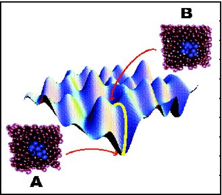
Figure 1: A model two-dimensional potential energy surface. The energy landscape is divided into basins of attraction, where the minima are the jammed states connected by pathways through saddle points. States A and B are typical packing configurations of 30 particles (in blue) with their periodic boundary systems.

II.2 Finding Stationary States

For the simplest system of $N$ structureless frictionless particles possessing no internal orientational and vibrational degrees of freedom, the potential energy function of this N-body system is $E(r_{1},\ldots,r_{N})$, where the vectors $r_{i}$ comprise position coordinates. As mentioned above, the most interesting points of a potential energy surface are the stationary points, where the gradient vanishes. Here we explain how to locate these stationary points. The algorithm follows well established methods in computational chemistry Wales1 . The procedure is analogous to finding the inherent structures wales0 of glassy systems. The algorithm employed, LBFGS algorithm, is also similar to the conjugate gradient method employed by O’ Hern ohern ; jpoint ; manypackings , differing in the fact that it does not require the calculation of the Hessian matrix at every time step. We make the source code in C$++$ available at http://www.jamlab.org and free to use together with all the packings generated in this study. The algorithm has been used in the short version of this article wang-epl and in a study of the PEL in Lennard-Jones glasses to reconstruct a network of stationary states and apply a percolation picture of the glass transition carmi .

II.3 General Method – Newton-Raphson Method

Consider the Taylor expansion of the potential energy, $E$, around a general point in configuration space, $r$,

$$E(r+h)=E(r)+g^{T}h+\frac{1}{2}h^{T}Hh+O(h^{3}),$$ (9)

where $g$ is the gradient, $g_{i}=\partial_{i}E$, $H$ is the Hessian matrix, $H_{ij}=\partial_{i}\partial_{j}E$, and $h$ is a small step vector that gives the displacement away from $r$.

By Eq. (9), the calculation of energy difference for a given step $h$ from the initial point $r$ is complicated. By selecting the eigenvectors of the Hessian matrix $e_{\alpha}$ as our local coordinates, we can simplify the Taylor expansion of Eq. (9) as:

$$\triangle E=E(r+h)-E(r)\approx\sum_{\alpha}(g_{\alpha}h_{\alpha}+\frac{\lambda_{\alpha}}{2}h_{\alpha}^{2}),$$ (10)

where $g=\sum_{\alpha}g_{\alpha}e_{\alpha}$, $h=\sum_{\alpha}h_{\alpha}e_{\alpha}$, $He_{\alpha}=\lambda_{\alpha}e_{\alpha}$, and $\lambda_{\alpha}$ is the eigenvalue of the Hessian matrix for component $\alpha$.

From Eq. (10), it is easy to see that the total change of energy could simply be the sum of the changes in each directions. This may help us to raise the energy in some directions and reduce the energy at others, and finally reach a stationary point. The length of each step components can be selected as the maximum change of energy:

$$h_{\alpha}=S_{\alpha}\frac{g_{\alpha}}{\lambda_{\alpha}},$$ (11)

as shown in Fig.2. The sign $S_{\alpha}=\pm 1$ in this formula depends on the choice of uphill or downhill direction. In fact, for $\lambda_{\alpha}>0$, it is possible to choose another step for the uphill case, since $\triangle E_{\alpha}$ increases as $|h_{\alpha}|$, but for large steps, the Taylor expansion Eq. (9) may breakdown. Therefore, it is important to control the step length. For $\lambda_{\alpha}<0$, we reach the opposite conclusion.

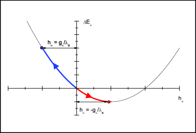
Figure 2: A schematic energy change curve for one component with $\lambda_{\alpha}>0$. We can select the downhill step as $h_{\alpha}=-\frac{g_{\alpha}}{\lambda_{\alpha}}$ to obtain a maximum energy change. The uphill step can not be too large since the Taylor expansion will not be accurate enough for the calculation. Here, the uphill step is chosen as $h_{\alpha}=\frac{g_{\alpha}}{\lambda_{\alpha}}$.

The stationary points can be separated into local minima and saddle points. Based on the eigenvalues of the Hessian matrix for the stationary point, the local minima are ordered as:

$$0\leq\lambda_{1}\leq\lambda_{2}\cdots\leq\lambda_{3N},$$ (12)

and for a saddle point of order $\alpha$:

$$\lambda_{1}\leq\cdots\leq\lambda_{\alpha}\leq 0\leq\lambda_{\alpha+1}\leq\cdots\leq\lambda_{3N}.$$ (13)

Generally, this algorithm searches for the nearest stationary point on the surface by following the opposite $(\lambda_{\alpha}\geq 0)$ and along $(\lambda_{\alpha}\leq 0)$ the various gradient directions.

II.4 Finding local minima – LBFGS algorithm

It is much easier to locate local minima than saddle points because, for the first, we only need to search downhill in every direction. At present one of the most efficient methods to search the local minima for large system is Nocedal’s limited memory Broyden-Fletcher-Goldfarb-Shanno algorithm (LBFGS) Nocedal1 ; wales0 . The LBFGS algorithm constructs an approximate inverse Hessian matrix from the gradients (first derivatives) which are calculated from previous points. Since it is only necessary to calculate the gradients at each searching step, the LBFGS algorithm increases the computational speed of the algorithm enormously.

In the Newton-Raphson method discussed above, the Hessian matrix of second derivatives is needed to be evaluated directly. Instead, the Hessian matrix used in LBFGS method is approximated using updates specified by gradient evaluations. The LBFGS algorithm code can be obtained from http://www.netlib.org/opt/index.html. Here we present a brief explanation of the algorithm

From an initial random point $r_{0}$ and an approximate Hessian matrix $H_{0}$ (in practice, $H_{0}$ can be initialized with $H_{0}=I$), the following steps are repeated until $r$ converges to the local minimum.

• Obtain a direction $h_{k}$ by solving: $H_{k}h_{k}=-\nabla E(r_{k})$.

• Perform a line search to find an acceptable step size $\gamma_{k}$ in the direction found in the first step, then update $r_{k+1}=r_{k}+\gamma_{k}h_{k}$.

• Set $s_{k}=\alpha_{k}h_{k}$.

• Set $y_{k}=\nabla E(r_{k+1})-\nabla E(r_{k})$.

• Set the new Hessian, $H_{k+1}=H_{k}+\frac{y_{k}y^{T}_{k}}{y^{T}_{k}s_{k}}-\frac{H_{k}s_{k}(H_{k}s_{k})^{T}}{s^{T}_{k}H_{k}s_{k}}$.

II.5 Finding saddles – Eigenvector following method

In the present study we do not make use of the saddle points. However, other studies using network theory to represent the PEL necessitate the links between minima through the saddle points carmi . For completeness, below we explain how to search for saddles. A particular powerful method for locating saddle points is the eigenvector following method Wales1 .

The eigenvector-following method, developed by Cerjan, Miller and others Miller1 ; Wales1 ; Grigera1 ; Doye1 ; Wales2 ; Walsh1 , consists of locating a saddle point from a local minimum. At each searching step towards a saddle point with $\alpha$ order, the directions are separated into two types: $\alpha$ uphill directions to maximization and $3N-\alpha$ downhill directions to minimization.

We follow the implementation of the eigenvector-following method by Grigera Grigera1 . We give a general description: at each searching step, a step size $h$ is calculated by the diagonalized Hessian matrix Grigera1 ; Wales2 ; Walsh1 :

$$h_{\alpha}=S_{\alpha}{2g_{\alpha}\over|\lambda_{\alpha}|\left(1+\sqrt{1+4g^{2}_{\alpha}/\lambda^{2}_{\alpha}}\right)},$$ (14)

where $\lambda_{\alpha}$ are the eigenvalues of the Hessian matrix and $g_{\alpha}$ are the components of the gradient in the diagonal base ($h_{\alpha}$ is set to 0 for the directions where $\lambda_{\alpha}=0$). The sign $S_{\alpha}=\pm 1$ is chosen by the order of the saddle point. For a saddle point of order $n$, the algorithm will set $S_{\alpha}=-1$ for $1\leq\alpha\leq n$ and $S_{\alpha}=1$ for $\alpha>n$.

When $g_{\alpha}\to 0$, the step size $h_{\alpha}$ converges to the Newton-Raphson step as Eq. (11):

$$h_{\alpha}=S_{\alpha}{g_{\alpha}\over\lambda_{\alpha}}+O(g_{\alpha}^{2}).$$ (15)

II.6 An Example

We generate a two dimensional soft-ball system in circular boundary, which contains 31 particles of equal radius, to illustrate the method of finding stationary and saddle points in the PEL. The interaction between particles (also the interaction between particles and wall) follows the Hertzian law powerlaw :

$$V(r_{i},r_{j})=\epsilon|r_{i}-r_{j}|^{\frac{5}{2}}$$ (16)

Here, $\epsilon$ is the interaction strength between particles $i$ and $j$. The volume fraction is $\phi=0.80$, which is closed to the jamming transition of $2d$ hard disks.

We first generate a random configuration, which is the initial point of the search of the minima. With the LBFGS method, we search the local minimum $A$ nearby this initial point. After the minimum $A$ is obtained, we apply the eigenvector following method to walk from the point $A$ on the potential energy surface to locate the transition state $C$ (here the transition state is a first order saddle). Finally, the minimum $B$ is located by applying LBFGS method again. Figure 3 shows configurations of two local minima (marked as red) and the transition state (marked as blue) between them.

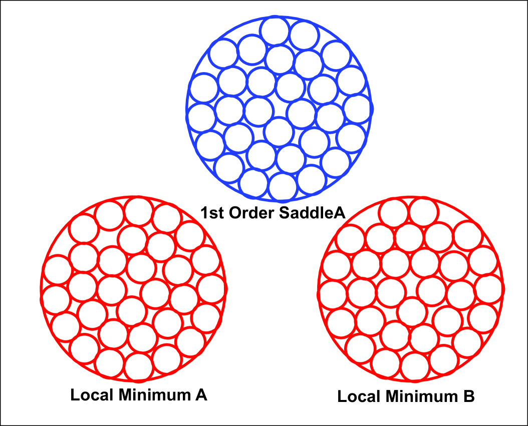
Figure 3: A two dimensional 31 particle system in a circular boundary. Three different configurations in this system are generated with different algorithms. The LBFGS method is applied to locate minima A and B. For saddle C which connects A and B, the eigenvector following method is used.

The pathway from minimum A to minimum B, passing by transition state C, is shown in Fig. 4. The pathway distance is the Euclidean distance,

$$d=\sqrt{(r^{\prime}-r)\dot{(}r^{\prime}-r)}=\sqrt{\sum_{i,\alpha}(r^{\prime}_{i,\alpha}-r_{i,\alpha})^{2}},$$ (17)

where $i=1,2,3$, $\alpha=1\cdots 3N$, $r^{\prime}$ is the coordinate of configuration passing along the searching method and $r$ is the coordinate of saddle $C$.

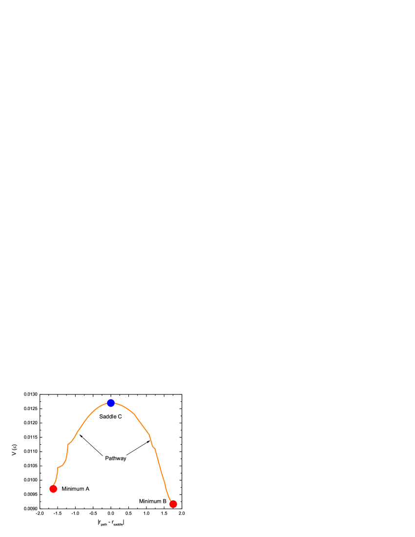
Figure 4: The pathway from minimum A to minimum B, passing by the saddle C, the x-coordinate is the distance from saddle C, the y-coordinate is the potential energy of the packing.

The dynamics from minimum to minimum can be represented as a walk on a network whose nodes correspond to the minima and where edges link those minima which are directly connected by a transition state. The work of Doye Doye2 provides an illustration of such a landscape network for a LJ energy surface. To characterize the topology of the landscape network, Doye Doye2 study small Lennard-Jones clusters to locate nearly all the minima and transition states on the potential energy landscape. The inherent structure network of such a system has a scale-free and small-world properties. In a companion study carmi we repeated the main results as Doye studied. The numbers of minima and transition states are expected to increase roughly as $N_{min}\sim e^{\alpha N}$ and $N_{st}\sim Ne^{\alpha N}$ respectively, where $N$ is the number of atoms in the cluster. Therefore, the largest network that we are able to consider is for a 14-atom cluster for which we have located 4158 minima and 90 738 transition states in agreement with the results of Doye. In the next Section we apply the above formalism to find the stationary states for a 3d granular system of Hertz spheres in a periodic boundary.

III System Information. Hertzian system of spheres

Next we calculate the density of jammed states $g(\Gamma,\phi)$ in the framework of the PEL formulation for a system of Hertz spheres. In the case of frictionless jammed systems, the mechanically stable configurations are defined as the local minima of the PEL jpoint ; manypackings .

The systems used for both, ensemble generation and molecular dynamic simulation, are the same. They are composed of 30 spherical particles in a periodic boundary box. The particles have same radius $R=5\mu m$ and interact via a Hertz normal repulsive force without friction. The normal force interaction is defined as powerlaw ; hmlaw1 ; hmlaw2 :

$$F_{n}=\frac{2}{3}~{}k_{n}R^{1/2}(\delta r)^{\delta},$$ (18)

where $\delta=3/2$ is the Hertz exponent, $\delta r=(1/2)[2R-|\vec{x}_{1}-\vec{x}_{2}|]>0$ is the normal overlap between the spheres and $k_{n}=4G/(1-\nu)$ is defined in terms of the shear modulus $G$ and the Poisson’s ratio $\nu$ of the material from which the grains are made. We use typical values for glass: $G=29$ GPa and $\nu=0.2$ and the density of the particles, $\rho=2\times 10^{3}$ kg/m³ powerlaw ; hmlaw2 . The interparticle potential energy is

$$E=\frac{2}{3}~{}\frac{k_{n}}{\delta+1}R^{1/2}(\delta r)^{\delta+1}.$$ (19)

The Hertz potential is chosen for its general applicability to granular materials. The results are expected to be independent of the form of the potential. Below, we apply the LBFGS algorithms Nocedal1 ; wales0 to find the local minima of the PES (zero-order saddles).

IV Ensemble Generation

In this section, we first explain the method to obtain geometrically distinct minima in the PEL to calculate the density of states. Then we show that the density of the states, $g(\Gamma,\phi)$, does not change significantly after sufficient searching time for the configurations.

In principle, if all local minima corresponding to the mechanically stable configurations of the PEL are obtained, the density of states $g(\Gamma,\phi)$ can be calculated. Such an exhaustive enumeration of all the jammed states requires that $N$ not be too large due to computational limits. On the other hand, in order to obtain a precise average pressure in the MD simulation, $\langle p\rangle_{\rm dyn}$, $N$ cannot be too small such that boundary effects are minimized. Considering these constraints, we choose a $30$ particle system.

In order to enumerate the jammed states at a given volume fraction $\phi$, we start by generating initial unjammed packings (not mechanically stable) performing a Monte Carlo (MC) simulation at a high, fixed temperature. The MC part of the method applied to the initial packings assumes a flat exploration of the whole PEL. Every MC unjammed configuration is in the basin of attraction of a jammed state which is defined as a local minimum in the PES with a positive definite Hessian matrix, that is a zero-order saddle. In order to find such a minimum, we apply the LBFGS algorithm provided by Nocedal and Liu Nocedal1 explained above. The PEL for each fixed $\phi$ likely includes millions of geometrically distinct minima by our simulation results. Therefore, an exhaustive search of configurations is computationally long; for a system of 30 particles it is impossible to find all the configurations with the current available computational power. However, we notice that it not crucial to find all the states, but rather a sufficiently accurate density of states. Therefore, we check that the number of found configurations has saturated after sufficient trials and that the density of states $g(\Gamma,\phi)$ has converged to a final shape under a prescribed approximation.

It is also important to determine if the local minima are distinct. Usually, the eigenvalues of the Hessian matrix at each local minimum can be used to distinguish these mechanically stable packings. Here, we follow this idea to compare minima to filter the symmetric packings. However, instead of calculating the eigenvalues of each packing, which is time consuming, we calculate a function of the distance between any two particles in the packing to improve search efficiency (for the LBFGS algorithm, we do not need to calculate the Hessian matrix). For each packing, we assign the function $Q_{i}$ for each particle:

$$Q_{i}=\sideset{}{}{\sum}_{1\leq j\leq N,\;\ j\neq i}{\tan}^{2}(\frac{\pi r_{ij}^{2}}{3L^{2}}),$$ (20)

where $r_{ij}$ is the distance between particles $i$ and $j$, $L$ is the system size and $N=30$. We list the $Q_{i}$ for each packing from minimum to maximum $\{Q_{i}\}(1\leq i\leq N)$. Since $Q_{i}$ is a higher order nonlinear function, we can assume that two packings are the same if they have the same list. The tolerance is defined as:

$$T=\sqrt{\frac{\sum_{\begin{subarray}{c}1\leq i\leq N\end{subarray}}(Q_{i}-Q^{{}^{\prime}}_{i})^{2}}{N^{2}}},$$ (21)

where $Q_{i}$ and $Q^{{}^{\prime}}_{i}$ are the corresponding values from the lists of two packings.

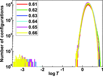
Figure 5: The distribution of the tolerance $T$ between any two packings at the given $\phi$. From the graph, the value of $T$ for which any two different packings are considered to be same is chosen to be $10^{-1}$, which is above the noise threshold and below the distribution of $T$.

Figure 5 shows the distributions of the tolerance $T$ for packings at different volume fractions. This figure suggests that two packings can be considered the same if $T\leq 10^{-1}$, which defines the noise level.

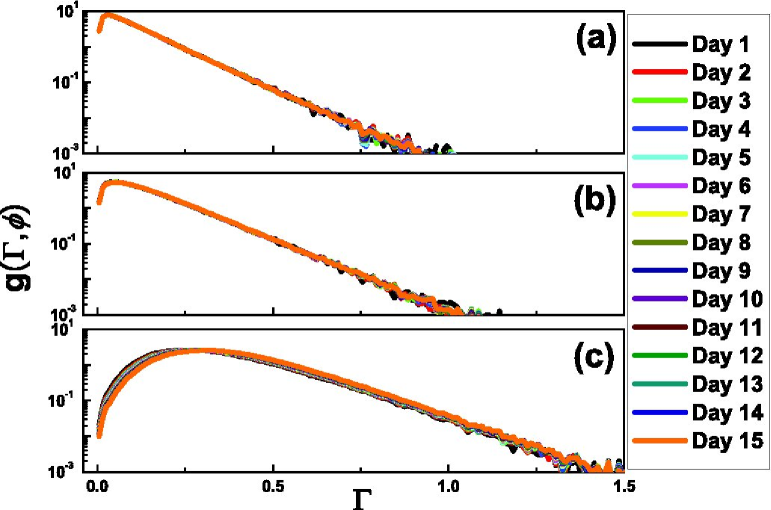
Figure 6: Log-log plot of the distribution of $g(\Gamma,\phi)$ for 15 searching days (a) at $\phi=0.609$, (b) at $\phi=0.614$, (c) at $\phi=0.625$. Different color in (a), (b), (c) corresponds to the different day. We find that after 15 days the distributions have converged.

From Fig. 6, we see that after one week of searching, $g(\Gamma,\phi)$ does not change significantly, since the initial packings are generated by a completely random protocol. We also calculate the probability of finding new mechanically stable states for different searching days, defined as $N_{\rm new}(i)/N_{\rm total}(i)$, where $N_{\rm new}(i)$ is the number of new configurations found on the $i$-th day and $N_{\rm total}(i)$ is the total number of configurations found in $i$ days. From Fig. 7, we see that, after one week searching, the probability of finding new configurations at different volume fractions seems to have converged in the linear plot. Figure 7b shows a detail of the actual number of new configurations found and $g(\Gamma,\phi)$ versus searching time in days suggesting convergence. However, the log-log plot of the inset in Fig. 7a indicates that the algorithm is still searching for new configurations; the power-law relation in the inset suggesting a neverending story. However, the main question is whether the observables have converged. A further test of convergence is obtained below in Fig. 14 where the value of the inverse angoricity is measured as a function of the searching time in days. This plot suggests that enough ensemble packings have been obtained to capture the features of $g(\Gamma,\phi)$ that give rise to the correct observables. We conclude that we have obtained an accurate enough density of states for this particular system size. Regarding system size dependence, the presented results are still $N$ dependent, although they started to converge for $N\sim 35$ and above, Fig. 8. More accurate calculations for large values of $N$ remain computationally impossible, but in our treatment the exact choice of $N$ is not as important as the consistency of the results between ensemble and MD, for a given $N$ value.

Figure 9 shows $g(\Gamma,\phi)$ versus $\Gamma$ for different volume fractions.

(a)

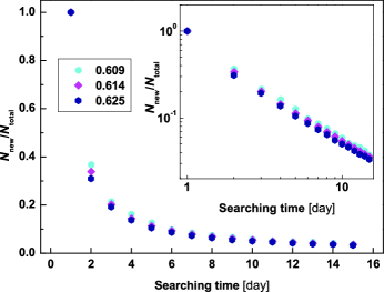
(b)

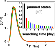
Figure 7: (a) The probability to find new configurations as a function of searching time. (b) Linear plot of the density of states as a function of searching time. Different colors indicate different days according to the inset. Inset shows the actual number of new configurations.

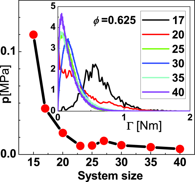
Figure 8: Dependence of the results on the system size. The average value of $p$ converges as early as $N\sim 25$ particles. The distribution $g(\Gamma,\phi)$ (inset) has not fully converged yet but its shape has converged after $N=35$ and the first moment does not change as indicated by the average $p$.

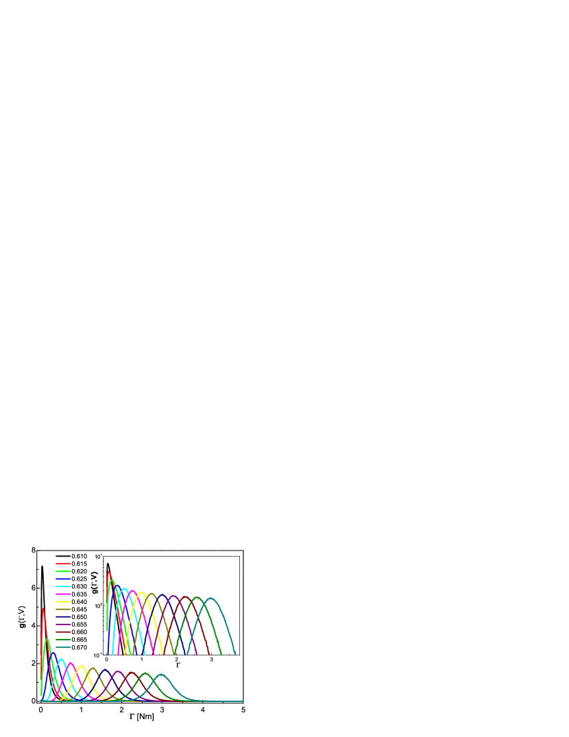
Figure 9: The density of states $g(\Gamma,\phi)$ as a function of internal virial $\Gamma$ for different volume fraction, $\phi$, ranging from 0.610 to 0.670. The inset shows the logarithmic distribution of $g(\Gamma,\phi)$. At low volume fraction ($\phi\lesssim 0.625$), the distributions are sharp and the tails of the distributions are exponential. At high volume fraction ($\phi\gtrsim 0.640$), the distributions are much broader and the tails are Gaussian.

V MD calculations

In order to analyze numerical results, we perform MD simulations to obtain $Z_{\rm dyn}$ and $\phi_{\rm dyn}$, which are herein considered real dynamics. The algorithm is described in detail in hmlaw2 ; compactivity ; forcebalance2 . Here, a general description is given: A gas of non-interacting particles at an initial volume fraction is generated in a periodically repeated cubic box. Then, an extremely slow isotropic compression is applied to the system. The compression rate is $\Gamma_{0}=5.9t_{0}^{-1}$, where the time is in units of $t_{0}=R\sqrt{\rho/G}$. After obtaining a state for which the pressure $p$ is a slightly higher than the prefixed pressure we choose, the compression is stopped and the system is allowed to relax to mechanical equilibrium following Newton’s equations. Then the system is compressed and relaxed repeatedly until the system can be mechanically stable at the predetermined pressure. To obtain the statical average of $Z_{\rm dyn}$ and $\phi_{\rm dyn}$, we repeat the simulation to get enough packing samples having statistically independent random initial particle positions. Here, 250 independent packings are obtained for each fixed pressure (see Fig. 10). $\phi=\langle\phi\rangle_{\rm dyn}$ and $\langle Z\rangle_{\rm dyn}$ are flat averages of these $250$ packings by

$$\langle\phi\rangle_{\rm dyn}=\frac{\sum_{1\leq i\leq 250}\phi_{i}}{250},$$ (22)

and

$$\langle Z\rangle_{\rm dyn}=\frac{\sum_{1\leq i\leq 250}Z_{i}}{250}.$$ (23)

(a)

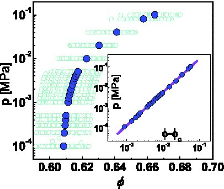
(b)

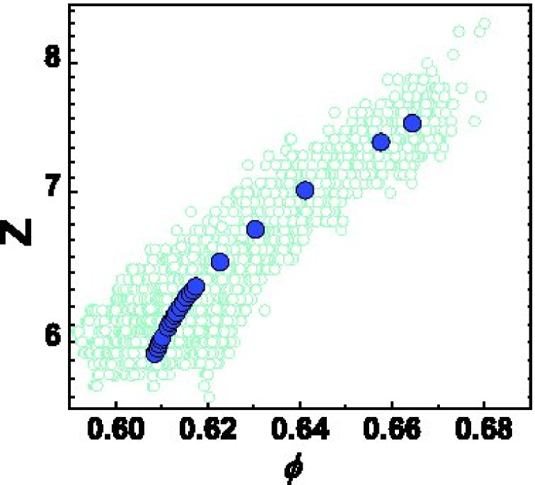
Figure 10: The cyan $\bigcirc$ is (a) $\phi_{\rm dyn}$ and (b) $Z_{\rm dyn}$ for every single packing obtained with MD and the blue $\bigcirc$ is $\langle\phi\rangle_{\rm dyn}$ and $\langle Z\rangle_{\rm dyn}$ average over the single packings for the system which are shown in the text of the paper.

From previous studies, it has been observed the pressure $p$ vanishes as power-law of $\phi$ when approaching the jamming transition as seen in Eq. (7) jpoint ; powerlaw . We obtain (Fig. 11)

$$\langle p\rangle_{\rm dyn}=p_{0}\,\,(\phi-\phi_{c})^{1.65}\,\,,$$ (24)

where $\phi_{c}=0.6077$ is the volume fraction corresponding to the isostatic point J jpoint ; powerlaw following Eq. (8) and $p_{0}=10.8{\rm MPa}$. This critical value $\phi_{c}$ and the exponent, $a=1.65$, are slightly different from the values obtained for larger systems ($a=\delta$) jpoint ; powerlaw . However, our purpose is to use the same system in the dynamical calculation and the exact enumeration for a proper comparison.

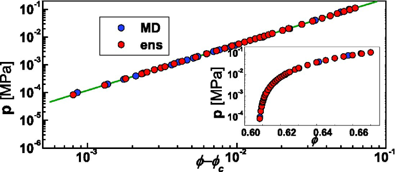
Figure 11: Scaling of pressure. The blue $\bigcirc$ shows the power-law relation for $\langle p\rangle_{\rm dyn}$ vs $\langle\phi\rangle_{\rm dyn}-\phi_{c}$ for the 30-particle system. Here, the pressure $\langle p\rangle_{\rm dyn}$ are average values obtained by 250 independent MD simulations. The red $\bigcirc$ is the pressure used to obtain the inverse angoricity $\alpha$ predicted by Eq. (24). The relatively small system size results in large fluctuations of the observables. In order to predict a precise relation for the system ($N=30$), sufficient independent samples of the packings are generated to calculate the precise average for observables. We prepare 250 independent packings for each $\phi$ to get enough statistical samples to obtain $\langle p\rangle_{\rm dyn}$ and $\langle Z\rangle_{\rm dyn}$ by statistical average. The inset shows a semi-log plot.

VI Angoricity Calculation

Since we obtain $g(\Gamma,\phi)$ and $\langle p\rangle_{\rm dyn}$ for each volume fraction $\phi$, we can calculate the inverse angoricity $\alpha$ by Eq. (3). The pressure $\langle p(\alpha,\phi)\rangle_{\rm ens}$ for a given $\phi$ is a function depending on $\alpha$ as:

$$\langle p(\alpha,\phi)\rangle_{\rm ens}=\frac{\int_{0}^{\infty}pg(\Gamma,\phi)e^{-\alpha\Gamma}{\rm d}\Gamma}{\int_{0}^{\infty}g(\Gamma,\phi)e^{-\alpha\Gamma}{\rm d}\Gamma}=\frac{\sum pe^{-\alpha\Gamma}}{\sum e^{-\alpha\Gamma}}.$$ (25)

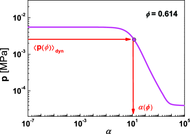
Figure 12: The numerical integration of Eq. (25) for $\phi=0.614$ is shown as the pink curve. We input the $\langle p\rangle_{\rm dyn}$ (pink $\bigcirc$ in the plot) and obtain the corresponding inverse angoricity $\alpha$.

Figure 12 shows the result of the numerical integration of Eq. (25) for a particular $\phi=0.614$ as a function of $\alpha$ using the numerically obtained $g(\Gamma,\phi)$ from Fig. 9. To obtain the value of $\alpha$ for this $\phi$, we input the corresponding measure of the pressure obtained dynamically $\langle p(\phi)\rangle_{\rm dyn}$ and obtain the value of $\alpha$ as schematically depicted in Fig. 12. The same procedure is followed for every $\phi$ (see Fig. 13) and the dependence $\alpha(\phi)$ is obtained.

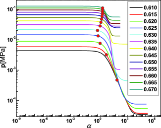
Figure 13: Calculation of $\alpha$ for several volume fractions $\phi$ as explained in detail in Fig. 12

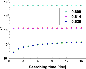
Figure 14: Calculation of inverse angoricity $\alpha$ as a function of searching time.

We also check the inverse angoricity $\alpha(\phi)$ using $g(\Gamma,\phi)$ for different searching days. to ensure the accuracy and convergence to the proper value. From Fig. 14, we can see that, after 10 days searching, $\alpha(\phi)$ is stable due to the fact that the density of state, $g(\Gamma,\phi)$, does not change significantly.

For each $\phi$ we use $g(\Gamma,\phi)$ to calculate $\langle p(\alpha)\rangle_{\rm ens}$ by Eq. (3). Then, we obtain $\alpha(\phi)$ by setting $\langle p(\alpha,\phi)\rangle_{\rm ens}=\langle p\rangle_{\rm dyn}$ for every $\phi$. The resulting equation of state $\alpha(\phi)$ is plotted in Fig. 15 and shows that the angoricity follows a power-law, near $\phi_{c}$, of the form:

$$A\propto(\phi-\phi_{c})^{\gamma},$$ (26)

with $\gamma=2.5$. The result is consistent with $\gamma=\delta+1.0$, suggesting that $A\propto\Gamma\propto F_{n}r$. For volume fraction much larger than $\phi_{c}$, the system’s input pressure $\langle p(\phi)\rangle_{\rm dyn}$ reaches the plateau at low $\alpha$ of the function $\langle p(\alpha,\phi)\rangle_{\rm ens}$ (see Fig. 13) and the corresponding $\alpha(\phi)$ becomes much smaller (the angoricity $A(\phi)$ becomes much larger), leading to large errors in the value of $A$ as $\phi$ becomes large. This might explain the plateau found in $A$ when $(\phi-\phi_{c})>2\times 10^{-2}$ as shown in Fig. 15.

Angoricity is a measure of the number of ways the stress can be distributed in a given volume. Since the stresses have a unique solution for a given configuration at the isostatic point, $\phi_{c}$, the corresponding angoricity vanishes. At higher pressure, the system is determined by multiple degrees of freedom satisfying mechanical equilibrium, leading to a higher stress temperature, $A$. The angoricity can also be viewed as a scale of stability for the system at different volume fractions. Systems jammed at larger volume fractions require higher angoricity (higher driving force) to rearrange.

(a)

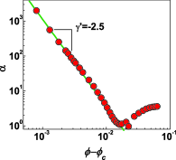
(b)

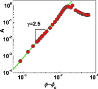
Figure 15: (a) Inverse angoricity $\alpha$ as a function of $\phi$-$\phi_{c}$. We find a power-law relation for system’s volume fraction $\phi$ near $\phi_{c}$. The solid line has a slope of -2.5. (b) The angoricity $A(=1/\alpha)$ vs $\phi$-$\phi_{c}$. To find $A$ accurately for system’s volume fraction $\phi$ much larger than $\phi_{c}$, becomes difficult due to the large fluctuations and finite size effects. In principle, we expect that the plateau of $A$ for large volume fraction $\phi$ might be related to the finite size of the sample. Indeed it is very difficult to estimate $\alpha$ since it falls in the plateau in Fig. 13.

VII Test of ergodicity

In principle, using the inverse angoricity, $\alpha$, from Eq. (26) we can calculate any macroscopic statistical observable $\langle B\rangle_{\rm ens}$ at a given volume by performing the ensemble average canonicaljam :

$$\langle B(\phi)\rangle_{\rm ens}=\frac{1}{{\mathcal{Z}}}\int_{0}^{\infty}B\,\,g(\Gamma,\phi)\,\,e^{-\alpha\Gamma}\,\,{\rm d}\Gamma.$$ (27)

We test the ergodic hypothesis in the Edwards’s ensemble by comparing Eq. (27) with the corresponding value obtained with MD simulations averaged over ($250$) sample packings, $B_{i}$, generated dynamically:

$$\langle B(\phi)\rangle_{\rm dyn}=\frac{1}{250}\sum_{i=1}^{250}B_{i}.$$ (28)

The comparison is realized by measuring the average coordination number, $\langle Z\rangle$, the average force and the distribution of interparticle forces. We calculate $\langle Z\rangle_{\rm ens}$ by Eq. (4) and $\langle Z\rangle_{\rm dyn}$ as in Eq. (28). Using $\alpha(\phi)$ for each volume fraction, we calculate $\langle Z\rangle_{\rm ens}$ by:

$$\langle Z(\phi)\rangle_{\rm ens}=\frac{\int_{0}^{\infty}Zg(\Gamma,\phi)e^{-\alpha\Gamma}{\rm d}\Gamma}{\int_{0}^{\infty}g(\Gamma,\phi)e^{-\alpha\Gamma}{\rm d}\Gamma}=\frac{\sum Ze^{-\alpha\Gamma}}{\sum e^{-\alpha\Gamma}}.$$ (29)

The average force $\langle\overline{F}\rangle_{\rm ens}$ is given by:

$$\langle\overline{F}(\phi)\rangle_{\rm ens}=\frac{\int_{0}^{\infty}\overline{F}g(\Gamma,\phi)e^{-\alpha\Gamma}{\rm d}\Gamma}{\int_{0}^{\infty}g(\Gamma,\phi)e^{-\alpha\Gamma}{\rm d}\Gamma}=\frac{\sum\overline{F}e^{-\alpha\Gamma}}{\sum e^{-\alpha\Gamma}},$$ (30)

where $\overline{F}$ is the average force for each ensemble packing. Finally, the force distribution $P_{\rm ens}(F/\overline{F})$ is given by:

$$P_{\rm ens}(F/\overline{F})=\frac{\int_{0}^{\infty}P(F/\overline{F})g(\Gamma,\phi)e^{-\alpha\Gamma}{\rm d}\Gamma}{\int_{0}^{\infty}g(\Gamma,\phi)e^{-\alpha\Gamma}{\rm d}\Gamma}=\frac{\sum P(F/\overline{F})e^{-\alpha\Gamma}}{\sum e^{-\alpha\Gamma}}.$$ (31)

Equations (29)–(31) are then compared with the dynamical measures for a test of ergodicity in Figs. 16 and 17.

(a)

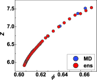
(b)

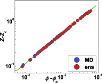
Figure 16: Test of ergodicity. (a) The blue $\bigcirc$ is the average coordination number $\langle Z\rangle_{\rm dyn}$ obtained by 250 independent MD simulations. The red $\bigcirc$ is the coordination number $\langle Z\rangle_{\rm ens}$ calculated by the ensemble for different volume fractions. Agreement between both measures supports the concept of ergodicity in the system. (b)The same as (a) but in a log-log plot. The blue $\bigcirc$ shows the power-law relations for $\langle Z\rangle_{\rm dyn}$-$Z_{c}$ vs $\langle\phi\rangle_{\rm dyn}$ -$\phi_{c}$ for 30-particle system with $\phi_{c}=0.6077$ and $Z_{c}=5.82$.

Figure 16a and 16b show that the two independent estimations of the coordination number agree very well: $\langle Z\rangle_{\rm ens}=\langle Z\rangle_{\rm dyn}$. The average inter-particle force $\overline{F}$ for a jammed packing is proportional to the pressure of the packing. We calculate $\langle\overline{F}\rangle_{\rm ens}$ and $\langle\overline{F}\rangle_{\rm dyn}$ and find that they coincide very closely (see Fig. 17a). The full distribution of inter-particle forces for jammed systems is also an important observable which has been extensively studied in previous works jpoint ; forcedist1 ; forcedist2 . The force distribution is calculated in the ensemble $P_{\rm ens}(F/\overline{F})$ by averaging the force distribution for every configuration in the PES. Figure 17b shows the distribution functions. The peak of the distribution shown in Fig. 17b indicates that the systems are jammed jpoint ; forcedist1 ; forcedist2 . Besides the exact shape of the distribution, the similarity between the ensemble and the dynamical calculations shown in Fig. 17b is significant. The study of $\langle Z\rangle$, $\langle\overline{F}\rangle$ and $P(F/\overline{F})$ reveals that the statistical ensemble can predict the macroscopic observables obtained in MD. We conclude that the idea of “thermalization” at an angoricity is able to describe the jamming system very well.

(a)

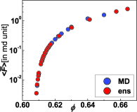
(b)

Figure 17: Test of ergodicity. (a) Comparison of $\langle\overline{F}\rangle_{\rm dyn}$ and $\langle\overline{F}\rangle_{\rm ens}$ for different volume fractions. (b) The comparison of selected distribution of force $P_{\rm dyn}(F/\overline{F})$ and $P_{\rm ens}(F/\overline{F})$ for different volume fractions.

The MD simulations performed so far are at a predetermined pressure $p$. For this case there is no difference between the force distribution $P(F/\overline{F})$ and $P(F/\langle\overline{F}\rangle)$ jpoint . On the other hand, a MD simulation at a given fixed volume fraction $\phi$, gives rise to different distributions. For each system with fixed $\phi$, the packings can have various pressure. This suggests that the force distribution for each packing scaled by the average force over all packings, $P(F/\langle\overline{F}\rangle)$, should be different from the force distribution scaled by the average force of that particular packing $P(F/\overline{F})$ ohern . We now proceed to investigate a constant volume MD, vMD simulation.

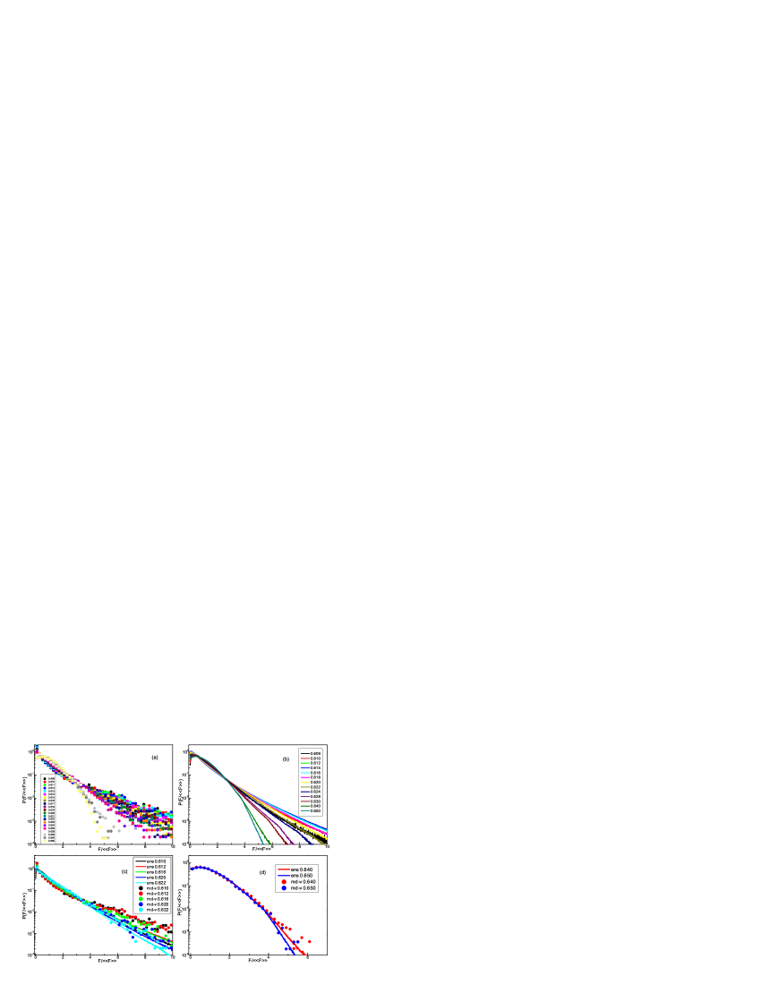
Figure 18: (a) The distribution of force $P_{\rm vMD}(F/\langle\overline{F}\rangle_{\rm vMD})$. (b) The distribution of force $P_{\rm ens}(F/\langle\overline{F}\rangle_{\rm ens})$. (c) and (d) The comparison of selected $P(F/\langle\overline{F}\rangle)$ between vMD and ensemble predicted by angoricity.

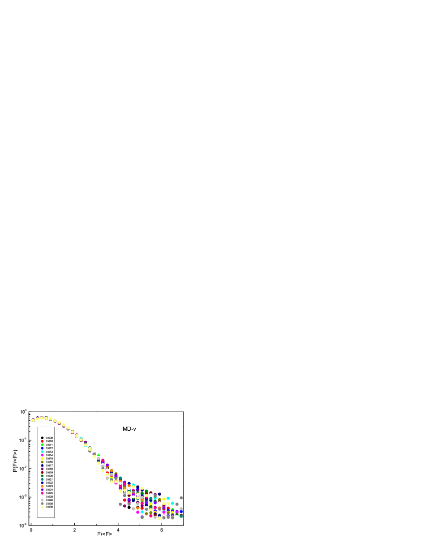
Figure 19: The distribution of forces, $P(F/\langle F\rangle)_{\rm vMD}$

The force distribution for vMD ensemble, $P_{\rm dyn}(F/\langle\overline{F}\rangle_{\rm dyn})$ is shown in Fig. 18a. From Fig. 18a, we find that the force distribution $P_{\rm dyn}(F/\langle\overline{F}\rangle_{\rm dyn})$ as a function of different volume fraction $\phi$ no longer collapse. At $\phi$ close to $\phi_{c}$, the average system force $\overline{F}$ for each packing changes dramatically. While at $\phi$ is much above $\phi_{c}$, the fluctuations of the average system force $\overline{F}$ decrease, then the force distribution $P_{\rm dyn}(F/\langle\overline{F}\rangle_{\rm dyn})$ changes continuously.

We can also calculate the force distribution $P_{\rm ens}(F/\langle\overline{F}\rangle_{\rm ens})$ in the ensemble average:

$$P_{\rm ens}(F/\langle\overline{F}\rangle_{\rm ens}=\frac{\int_{0}^{\infty}P(F/\langle\overline{F}\rangle_{\rm ens})g(\Gamma,\phi)e^{-\alpha\Gamma}{\rm d}\Gamma}{\int_{0}^{\infty}g(\Gamma,\phi)e^{-\alpha\Gamma}{\rm d}\Gamma},$$ (32)

where $\langle\overline{F}\rangle_{\rm ens}$ is the overall average $\overline{F}$ of the ensemble.

From Fig. 18b, we find the same tendency as obtained in MD simulation. Furthermore, we check the distribution of force $P(F/\langle F\rangle)$ for our vMD system (see Fig. 19). We see that $P(F/\langle F\rangle)$ for different volume fraction $\phi$ collapses very well similarly to those obtained from the predetermined pressure system. This result suggests that $P(F/\langle F\rangle)$ is a global quantity that can be used to verify if the system is jammed or not ohern .

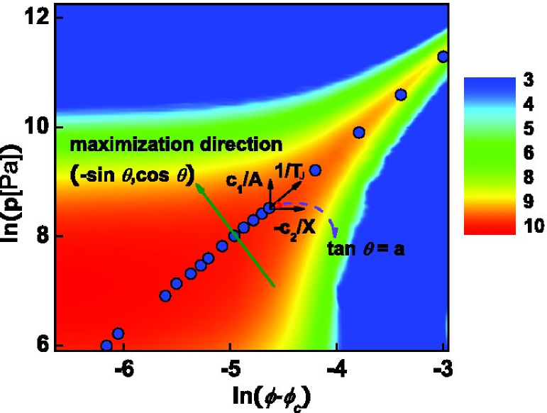
Figure 20: Microcanonical calculations. The entropy surface $S(\ln(\phi-\phi_{c}),\ln p)$. The color bar indicates the value of the entropy. The superimposed blue $\bigcirc$ is $\langle p(\phi)\rangle_{\rm dyn}$ from MD calculations as in Fig. 11. The olive arrow line indicates the maximization direction of the entropy $(-\sin\theta,\cos\theta)$. Following this direction, the entropy is maximum at the point $(\ln(\langle\phi\rangle_{\rm dyn}-\phi_{c}),\ln\langle p\rangle_{\rm dyn})$, corroborating the maximum entropy principle.

VIII Thermodynamic analysis of the jamming transition

So far we have considered how the angoricity determines the pressure fluctuations in a jammed packing at a fixed $\phi$. The role of the compactivity in the jamming transition can be analyzed in terms of the entropy which is easily calculated in the microcanonical ensemble from the density of states. Figure 20 shows the entropy of the system as a function of $(p,\phi)$ in phase space:

$$S=\ln(\Omega(p,\phi)).$$ (33)

Here $\Omega$ is the number of states which is the unnormalized version of $g(\Gamma,\phi)$. It is important to note that Fig. 20 shows the non-equilibrium entropy, in the Edwards sense. At the Edwards equilibrium, the entropy is maximum respect to changes in $\phi$ and $\Gamma$. We will now see how the jammed system verifies the principle of maximum entropy.

We analyze the entropy surface $S(\ln(\phi-\phi_{c}),\ln p)$ plotted versus $(\ln(\phi-\phi_{c}),\ln p)$ in Fig. 20. When we plot superimposed the MD-obtained curve $\langle p(\phi)\rangle_{\rm dyn}$ we see that the MD values pass along the maximum of the entropy surface constrained by the coupling between $p$ and $\phi$, Eq. (8) (such a curve is superimposed to the entropy surface in Fig. 20). Due to the coupling through the contact force law, the maximization of entropy is not on $p$ or $\phi$ alone but on a combination of both. The entropy $S$ reaches a maximum at the point $S(\ln(\langle\phi\rangle_{\rm dyn}-\phi_{c}),\ln\langle p\rangle_{\rm dyn})$ when we move along the direction perpendicular to the jamming curve $\langle p(\phi)\rangle_{\rm dyn}$ (see the maximization direction in Fig. 20). This is a direct verification of the second-law of thermodynamics: the dynamical measures maximize the entropy of the system.

We can use this result to obtain a relation between angoricity and compactivity and show how a new “jamming temperature” $T_{\rm J}$ and the corresponding jamming “heat” capacity $C_{\rm J}$ can describe the jamming transition.

From the power-law relation $p=\Gamma/V\propto(\phi-\phi_{c})^{a}$, we have:

$$\ln p=\ln p_{0}+a\ln(\phi-\phi_{c}),$$ (34)

where $p_{0}$ is the constant depending on the system.

Figure 20 indicates that the jammed system always remain at the positions of maximal entropy,

$$\delta S=0,$$ (35)

in the direction ($-\sin\theta$,$\cos\theta$), perpendicular to the jamming power-law curve and the slope

$$\tan\theta=a.$$ (36)

In order to further analyze this result, we plot the entropy distribution along the direction ($-\sin\theta$,$\cos\theta$) in Fig. 21. We see that the entropy of the corresponding jammed states remains at the peak of the distributions along ($-\sin\theta$,$\cos\theta$). This is clear when we plot the value of $(p,\phi)$ from MD simulations in the plot of $S$ in Fig. 21, blue dot. Except for volumes very close to jamming, the MD coincides with the maximum of $S$ when taken along ($-\sin\theta$,$\cos\theta$). We notice that the maximization is quite accurate for large volume fractions. For $\phi$ close to jamming deviations are seen. We cannot rule out that these deviations are finite size effects. The deviations for small $\phi$ (Fig. 21) remains to be studied. They could be due to finite size effects or due to the fact that the value of $\phi_{c}$ is different for the MD results and the microcanonical ensemble $S$ due to the small size of the system. In general, this plot verifies the maximum entropy principle in this particular direction. An analogous plot where the entropy is shown as a function of $\phi$ but along the horizontal direction (or along the vertical direction, $\Gamma$) shows that the MD entropy is not maximal along these two directions.

Thus, the maximization of entropy is not on $\Gamma$ or $V$ alone, but on a combination of both. This means that the entropy $S(\ln(\langle\phi\rangle_{\rm dyn}-\phi_{c}),\ln\langle p\rangle_{\rm dyn})$ is maximum along the direction of ($-\sin\theta$,$\cos\theta$) and the slope for the entropy of the jamming power-law curve along this direction ($-\sin\theta$,$\cos\theta$) is $0$ (see Fig. 22), that is,

$$\frac{\partial S}{\partial\ln(\phi-\phi_{c})}\sin\theta=\frac{\partial S}{\partial\ln p}\cos\theta.$$ (37)

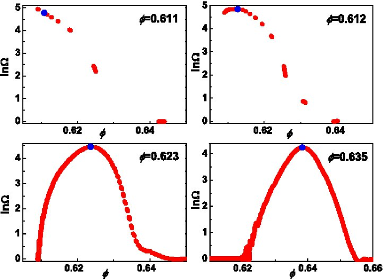
Figure 21: The non-equilibrium entropy $S(\ln p,\ln(\phi-\phi_{c}))$ along the direction $(-\sin\theta,\cos\theta)$ for different jamming ensemble points. The blue $\bigcirc$ represents the entropy of the jammed system obtained from MD. We see that closely follows the maximum of $S$ for all the volume fractions except very close to the jamming point where the blue point does not coincide with the maximum of $S$. It remains to be studied if this deviation is a finite size effect, or it could be due to a different value of $\phi_{c}$ between simulations and microcanonical ensemble.

Figure 22: The representation of the maximization analysis $\delta S=0$ along the direction $(-\sin\theta,\cos\theta)$ for one point in the jamming power-law curve. Here $c_{1}=\Gamma$ and $c_{2}=(\phi-\phi_{c})(NV_{g}/\phi^{2})$.

By the definition of angoricity $A=\partial\Gamma/\partial S$ and compactivity $X=\partial V/\partial S$, we have:

$$\frac{\partial S}{\partial\ln p}=p\frac{\partial S}{\partial p}=\Gamma\frac{\partial S}{\partial\Gamma}=\frac{\Gamma}{A}=\frac{c_{1}}{A},$$ (38)

$$\begin{split}\frac{\partial S}{\partial\ln(\phi-\phi_{c})}=&(\phi-\phi_{c})\frac{\partial S}{\partial\phi}=(\phi-\phi_{c})\frac{\partial V}{\partial\phi}\frac{1}{X}=\\ =&-(\phi-\phi_{c})\frac{NV_{g}}{\phi^{2}}\frac{1}{X}=-\frac{c_{2}}{X},\end{split}$$ (39)

where $\phi=NV_{g}/V$, $c_{1}=\Gamma$ and $c_{2}=(\phi-\phi_{c})(NV_{g}/\phi^{2})$.

By Eq. (38) and Eq. (39), we can simplify Eq. (37):

$$\frac{c_{1}}{A}+a\frac{c_{2}}{X}=0.$$ (40)

The relation between $X$ and $A$ can be obtained then (Fig. 22):

$$X=-a\frac{c_{2}}{c_{1}}A=-a\frac{\phi-\phi_{c}}{p\phi}A.$$ (41)

From Eq. (41) we obtain that: $X\propto-(\phi-\phi_{c})^{1+a-\gamma}/\phi$ and near $\phi_{c}$:

$$X\sim-(\phi-\phi_{c})^{2}.$$ (42)

We notice that the compactivity is negative near the jamming transition. A negative temperature is a general property of systems with bounded energy like spins fluctuation : the system attains the larger volume (or energy in spins) at $\phi_{c}$ when $X\to 0^{-}$ and not $X\to+\infty$ [The bounds $\phi_{c}\leq\phi\leq 1$ imply that the jamming point at $X\to 0^{-}$ is “hotter” than $X\to+\infty$. At the same time $A\to 0^{+}$ since the pressure vanishes].

We conclude that, $A$ and $X$ alone cannot play the role of temperature, but a combination of both determined by entropy maximization satisfying the coupling between stress and strain. Instead, there is an actual “jamming temperature” $T_{\rm J}$ that determines the direction $(-\sin\theta,\cos\theta)$ in the $\log-\log$ plot of Fig. 20 along the jamming equation of state (see Fig. 22). By maximizing the entropy along this direction we obtain the “jamming temperature” $T_{\rm J}$ as a function of $A$ and $X$:

$$\frac{1}{T_{\rm J}}=\frac{c_{1}}{A}\sin\theta-\frac{c_{2}}{X}\cos\theta=\cos\theta(a\frac{c_{1}}{A}-\frac{c_{2}}{X}).$$ (43)

That is:

$$\begin{split}T_{\rm J}=&\frac{A\sin\theta}{c_{1}}=-\frac{X\cos\theta}{c_{2}}=\frac{\sin\theta}{\Gamma}A=\\ =&\frac{a}{\sqrt{1+a^{2}}}\frac{A}{\Gamma}\sim(\phi-\phi_{c})^{\gamma-a}\sim(\phi-\phi_{c}).\end{split}$$ (44)

Thus, the temperature vanishes at the jamming transition.

Furthermore, the “jamming energy” $E_{\rm J}$, corresponding to the “jamming temperature” $T_{\rm J}$ in Eq. (43), has the relation as below:

$$\begin{split}{\rm d}E_{\rm J}&=T_{\rm J}{\rm d}S\\ &=T_{\rm J}\frac{\partial S}{\partial\ln(\phi-\phi_{c})}{\rm d}\ln(\phi-\phi_{c})+T_{\rm J}\frac{\partial S}{\partial\ln p}{\rm d}\ln p\\ &=(-\frac{X\cos\theta}{c_{2}})(-\frac{c_{2}}{X}){\rm d}\ln(\phi-\phi_{c})+\frac{A\sin\theta}{c_{1}}\frac{c_{1}}{A}{\rm d}\ln p\\ &=\cos\theta{\rm d}\ln(\phi-\phi_{c})+\sin\theta{\rm d}\ln p\\ &=(\cos\theta+\sin\theta\tan\theta){\rm d}\ln(\phi-\phi_{c})\\ &=\frac{{\rm d}\ln(\phi-\phi_{c})}{\cos\theta}.\end{split}$$ (45)

That is,

$${\rm d}E_{\rm J}=\sqrt{a^{2}+1}{\rm d}\ln(\phi-\phi_{c}),$$ (46)

and

$$E_{\rm J}=(\sqrt{a^{2}+1})\ln(\phi-\phi_{c}).$$ (47)

By the definition of “heat” capacity, we obtain two jamming capacities as the response to changes in $A$ and $X$:

$$\begin{array}[]{rl}C_{\rm\Gamma}\equiv&\partial\Gamma/\partial A\sim(\phi-\phi_{c})^{-1}\sim A^{-2/5},\\ C_{\rm V}\equiv&\partial V/\partial X\sim(\phi-\phi_{c})^{-1}\sim|X|^{-1/2}.\end{array}$$ (48)

The jamming capacity $C_{\rm J}$ can be obtained as:

$$C_{\rm J}=T_{\rm J}\frac{\partial S}{\partial T_{\rm J}}=T_{\rm J}\frac{\partial S}{\partial\ln p}\frac{\partial\ln p}{\partial T_{\rm J}}+T_{\rm J}\frac{\partial S}{\partial\ln(\phi-\phi_{c})}\frac{\partial\ln(\phi-\phi_{c})}{\partial T_{\rm J}}.$$ (49)

Finally, with Eq. (37)–(39), the capacity $C_{\rm J}$ can be calculated:

$$C_{\rm J}=T_{\rm J}(\frac{c_{1}}{A}-\frac{c_{2}}{aX})\frac{\partial\ln p}{\partial T_{\rm J}}=T_{\rm J}\frac{1+a^{2}}{a^{2}}\frac{c_{1}}{A}\frac{\partial\ln p}{\partial T_{\rm J}}.$$ (50)

Since $T_{\rm J}\sim(\phi-\phi_{c})$ and $p\sim(\phi-\phi_{c})^{1.5}$, we obtain

$$C_{\rm J}\sim(\phi-\phi_{c})^{-1}.$$ (51)

From Eq. (48), the jamming capacities diverge at the jamming transition as $A\to 0^{+}$ and $X\to 0^{-}$. However, this result does not imply that the transition is critical since from fluctuation theory of pressure and volume fluctuation we obtain:

$$\begin{split}\langle(\Delta\Gamma)^{2}\rangle=A^{2}C_{\rm\Gamma}\sim A^{1.6},\\ \langle(\Delta V)^{2}\rangle=X^{2}C_{\rm V}\sim|X|^{1.5}.\end{split}$$ (52)

Thus, the pressure and volume fluctuations near the jamming transition do not diverge, but instead vanish when $A\rightarrow 0^{+}$ and $X\rightarrow 0^{-}$. From a thermodynamical point of view, the transition is not of second order due to the lack of critical fluctuations. As a consequence, no diverging static correlation length from a correlation function can be found at the jamming point. However, other correlation lengths of dynamic origin may still exist in the response of the jammed system to perturbations, such as those imposed by a shear strain or in vibrating modes mode1 ; mode2 . Such a dynamic correlation length would not appear in a purely thermodynamic static treatment as developed here. We note that static anisotropic packings can be treated in the present formalism by allowing the inverse angoricity to be tensorial canonicaljam .

The intensive jamming temperature Eq. (44) gives use to a jamming effective energy $E_{\rm J}$ as the extensive variable satisfying $T_{\rm J}=\partial E_{\rm J}/\partial S$ and a full jamming capacity $C_{\rm J}\sim(\phi-\phi_{c})^{-1}$, which also diverges at jamming. However, the fluctuations of $E_{\rm J}$ defined as $\langle(\Delta E_{\rm J})^{2}\rangle=T_{\rm J}^{2}C_{\rm J}\sim T_{\rm J}$ has the same behavior as the fluctuations of volume and pressure, vanishing at the jamming transition $T_{\rm J}\to 0^{+}$ [$A\to 0^{+}$ in Eq. (44)].

IX Comparison with O’Hern et al.

The results so far show a general agreement between MD and the ensemble average. These include the maximum entropy principle and ergodicity. We now turn to a comparison with similar simulations done by O’Hern et al. ohern ; manypackings . These studies perform an exhaustive search of all configurations in the PEL of frictionless particles similarly as in the present paper. However, they find that the microstates are not equiprobable, i.e., microstates with the same pressure and volume fraction (pressure is fixed at zero since only hard sphere states are of interest) do not have the same probability when sampled by a given algorithm. Furthermore, experimental studies of equilibration between two systems leche , suggests that a hidden variable is necessary to describe the microstates, further supporting the results of ohern . The applicability of the microcanonical ensemble is based on the fact that the microstates are defined by $(\Gamma,\phi)$. Thus, the fact that the states are not equiprobable implies that there must be an extra variable needed to describe their probabilities. Therefore, ergodicity and the maximum entropy principle, which are downstream from equiprobability, are not supposed to hold, in disagreement with the results shown in the present paper.

To investigate this situation, we repeat the same calculations as in ohern with our algorithms. We first rule out subtleties related to algorithmic dependent results in sampling the space of configurations. We use our 30 particles system and use $\phi=0.61$ very close to jamming and $\Gamma=0$ to look for the hard sphere packings. We search for the jammed configurations as above. We recall that the sampling of the space of configurations is not complete due to the relatively large system size but represent a good sampling as discussed above. Ref. ohern uses a different system of 14 particles in 2d for which 248,900 configurations are found exhaustively sampling the phase space (which is estimated to have $\sim 371,500$ states). These simulations correspond to a system with periodic boundary conditions for which a larger space is expected than the close boundary-system of Section II.6. However, these differences do not affect the conclusions below.

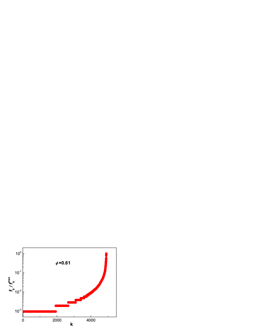
Figure 23: Sampling probability of each microstate $f_{k}$ identified by its rank $k$ fro low to high. Results are for a system of 30 particles at $\phi=0.61$ and a narrow set of pressures around 0.

We start by measuring $f_{k}$ which is the probability to find a given microstate $k$ as defined by ohern : each packing can be obtained many times during a search and therefore $f_{k}$ measures the probability for which each packing occurs. The main result of ohern is that $f_{k}$ differs by many orders of magnitude for states with fixed $(\Gamma,\phi)$. Indeed, even configurations which are visually very similar can be $10^{6}$ more frequent, see Fig. 1 of ohern .

Figure 23 shows $f_{k}$ sorted as a function of $k$, the rank, as in ohern . This plot reproduces the results of ohern in our system. For a fixed pressure and volume there are many states with a large difference in their probability. The least probable states are 10^-3 less probable than the most probable state showing a breakdown of equiprobability. The question is how to interpret the results of ergodicity in the light of the failure of equiprobability and whether there is a need for an extra variable to describe the microstates.

We first mention the issue of the small system size. It is quite possible that the low probability states will completely disappear in the thermodynamic limit and the ones remaining are the most probable ones with equal probability. Indeed, the flat average assumption is only valid in the thermodynamic limit and simply says that even if there exists less probable states ($10^{-3}$ less probable) then they will be irrelevant in the ensemble average, thus only the most probable and flat states are important.

(a)

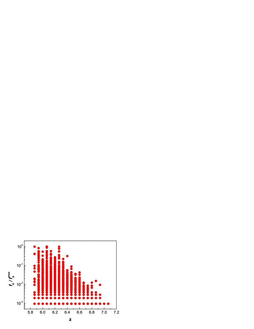
(b)

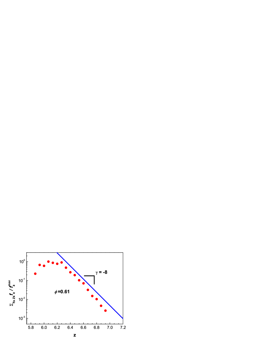
Figure 24: (a) Sampling probability of each microstate $f_{k}$ as a function of the coordination number $Z_{k}$ of each microstate. (b) Plot of $\ln(\sum_{{\rm fix}Z_{k}}f_{k}/f_{k}^{max})$ versus $Z_{k}$ showing an exponential decay consistent with the density of states proposed in compactivity .

We have done simulations with $N=$14 particles and found that the least probable states are $10^{-5}$ less probable than the most probable states. Comparing with the factor $10^{-3}$ for $N=30$, may indicate that the system size may take care of the non-equiprobability problem. However, calculations for larger system to fully test this assertion are out of the range of current and near future computational power.

Second, we notice that the coordination number is also important to define the jammed states. Figure 24 plots the same states as Fig. 23 but as a function of $Z_{k}$, the coordination number of microstate $k$. The most probable states satisfy:

$$f_{k}(Z_{k})\sim e^{-8Z_{k}}.$$ (53)

Furthermore, if we sum up all the states for a given $Z_{k}$ and plot $\log(\sum_{{\rm fix}Z_{k}}f_{k})$ vs $Z_{k}$ we obtain Eq. (53) as seen in Fig. 24b. This result does not mean that $Z_{k}$ is the hidden variable but rather Eq. (53) provides the density of states proposed in compactivity in the thermodynamics calculation of the random close packing of spheres. Indeed, we have predicted that the density of states $g(z)=h_{z}^{z}$, with $h_{z}$ playing the role of a Planck constant defining the minimum size in the volume landscape. According to Eq. (53), this prediction is satisfied in average with $h_{z}=e^{-8}$ which is a small number as expected.

This result indicates that some variability in the probabilities of the microstates is expected from the fluctuations in the coordination number of each microstate. In Appendix A we elaborate an extension of the framework of compactivity to incorporate fluctuations in $Z$ that are neglected in compactivity . The purpose is to test whether the RCP and jamming transition are affected by these fluctuations. We find that the results are consistent with those found in compactivity .

We notice that for a fix $Z_{k}$ there are still many marginal states with very small probabilities as seen in Fig. 24a. If these states do not completely disappear in the thermodynamic limit, then they need to be explained. We end this discussion by providing a possible explanation for the existence of these states.

The numerical breakdown of equiprobability might be related to the fact that the found packings are not indistinguishable. Indeed, we ignore the rotation and translation symmetries of the packing in order to make the numerical search possible. However, for the Edwards flat hypothesis, these packings should be assumed different. Once we breakdown the rotational symmetry, there would be many similar packings. The high degeneracy of the high symmetric packings may be responsible for the uneven distribution, which would be, in this case, simply artificial.

For instance, consider two packings with 4 particles: (a) a square packing with each particle on the corner and (b) a triangle with each particle in each corner plus one in the center.

For both packings there are 4! = 24 different permutations, which should be considered as 24 different packings, in principle. However, since we can rotate the square packing by 90 degree and obtain the same one, there are only 24/4 = 6 distinguishable packings. Similarly, for the triangle, there are 24/3 = 8 distinguishable packings. The probability between (a) and (b) is uneven (6:8) if we assume that each distinguishable packing is equal-probable. Therefore, different symmetries of the packings may contribute to the unequal probabilities that we measure in the algorithms.

Therefore, if the Edwards assumption is correct, $f_{k}$ should be proportional to $S_{k}$, where $S_{k}$ is the order of the symmetry group (point group) of the packing $k$, since there are $S_{k}$ degenerations (same packing if particles are identical). This conjecture needs extra evaluation of the symmetry of each packing. For instance, the translation invariance is important, and for cubic periodic boundary, it is also important to include the symmetry of cubic point group C_3h.

We do not investigate this conjecture but rather provide the codes and packings in http://jamlab.org to do that. Since the 3d case is complicated, one might try the 2d system first to easily visualize different packings. A simple question is: given two packings with different frequencies, how do they look like ohern ? Would be the high symmetric one visited more, or inversely?

X Conclusion

We have demonstrated that the concept of “ thermalization ” at a compactivity and angoricity in jammed systems is reasonable by the direct test of ergodicity. The numerical results indicate that the full canonical ensemble of pressure and volume describes the observables near the jamming transition quite well. From a static thermodynamic viewpoint, the jamming phase transition does not present critical fluctuations characteristic of second-order transitions since the fluctuations of several observables vanish approaching jamming. The lack of critical fluctuations is respect to the angoricity and compactivity in the jammed phase $\phi\to\phi_{c}^{+}$, which does not preclude the existence of critical fluctuations when accounting for the full range of fluctuations in the liquid to jammed transition below $\phi_{c}$. Thus, a critical diverging length scale might still appear as $\phi\to\phi_{c}^{-}$ glass0 , which has been recently observed by experiment glass1 .

In conclusion, our results suggest an ensemble treatment of the jamming transition. One possible analytical route to use this formalism would be to incorporate the coupling between volume and coordination number at the particle level found in compactivity ; j1 together with similar dependence for the stress to solve the partition function. This treatment would allow analytical solutions for the observables with the goal of characterizing the scaling laws near the jamming transition.

Acknowledgements: We thank NSF-CMMT and DOE-Geosciences Division for financial support and L. Gallos for discussions.

Appendix A Microstates and Fluctuations in coordination number

Here, we develop a $Z$-ensemble for hard spheres in the limit of zero angoricity. In the main test we found that fluctuations in $Z$ may account for certain variability in the probability of microstates. Here we investigate whether this variability affect the existence of RCP and the jamming point. We develop a partition function in Edwards ensemble to study the dependence of RCP on this type of fluctuations.

The partition function is

$$\mathcal{Z}=\int\ldots\int_{Nz_{min}<\sum z_{i}<Nz_{max}}\prod_{i}e^{-(z_{i}/z^{*}+\beta\kappa/z_{i})}dz_{i},$$ (54)

where $z_{min}=Z$ and $z_{max}=6$, $\beta=1/X$, and $\kappa=2\sqrt{3}$. We follow the notation and concepts from compactivity ; j1 ; j2 ; j3 . We define $x=(\sum_{i}z_{i})/N$, thus:

$$\mathcal{Z}=\int_{z_{min}}^{z_{max}}P(x)dx,$$ (55)

where

$$P(x)\equiv\int_{0}^{\infty}\ldots\int_{0}^{\infty}\prod_{i}e^{-(z_{i}/z^{*}+\beta\kappa/z_{i})}\delta\left(x-\frac{1}{N}\sum_{i}z_{i}\right)dz_{i},$$ (56)

where $z^{*}=1/8$ according to Fig. 24b. We consider the inverse Fourier transform of $P_{x}(f)$:

$$\begin{split}\mathcal{F}_{f}^{-1}[P_{x}(f)]\equiv\int_{-\infty}^{\infty}e^{2\pi ifX}P(x)dx=\int_{0}^{\infty}\ldots\int_{0}^{\infty}\prod_{i}e^{-(z_{i}/z^{*}+\beta\kappa/z_{i})}e^{2\pi if\sum z_{i}/N}dz_{i}=\\ =\left[\int_{0}^{\infty}e^{-(z/z^{*}+\beta\kappa/z)}e^{2\pi ifz/N}dz\right]^{N}=\left\{\int_{0}^{\infty}\left[1+\left(\frac{2\pi ifz}{N}\right)+\frac{1}{2}\left(\frac{2\pi ifz}{N}\right)^{2}+\ldots\right]e^{-(z/z^{*}+\beta\kappa/z)}\right\}^{N}.\end{split}$$ (57)

Since

$$\int_{0}^{\infty}x^{n}e^{-\frac{a}{2}(x+1/x)}dx=2K_{n}(a),$$ (58)

where $K_{n}(a)$ is the modified Bessel function of the second kind. By taking the coupling constant

$$\begin{split}B\equiv\beta\kappa/z^{*},\\ a\equiv 2B^{1/2},\\ z=B^{1/2}z^{*}x.\end{split}$$ (59)

Then:

$$\int_{0}^{\infty}z^{n}e^{-(z/z^{*}+\beta\kappa/z)}dz=2{z^{*}}^{n+1}B^{(n+1)/2}K_{n}(2B^{1/2}).$$ (60)

Thus,

$$\begin{split}\mathcal{F}_{f}^{-1}[P_{X}(f)]&=(2z^{*})^{N}\left[B^{1/2}K_{0}(2B^{1/2})+\left(\frac{2\pi ifz^{*}}{N}\right)BK_{1}(2B^{1/2})+\frac{1}{2}\left(\frac{2\pi ifz^{*}}{N}\right)^{2}B^{3/2}K_{2}(2B^{1/2})+O(N^{-3})\right]^{N}\\ &=(2z^{*})^{N}\exp\left\{N\ln\left[B^{1/2}K_{0}(2B^{1/2})+\left(\frac{2\pi ifz^{*}}{N}\right)BK_{1}(2B^{1/2})+\frac{1}{2}\left(\frac{2\pi ifz^{*}}{N}\right)^{2}B^{3/2}K_{2}(2B^{1/2})+O(N^{-3})\right]\right\}\\ &=(2z^{*}B^{1/2}K_{0}(2B^{1/2}))^{N}\exp\left\{N\ln\left[1+\left(\frac{2\pi ifz^{*}}{N}\right)\frac{K_{1}(2B^{1/2})}{K_{0}(2B^{1/2})}B^{1/2}+\frac{1}{2}\left(\frac{2\pi ifz^{*}}{N}\right)^{2}\frac{K_{2}(2B^{1/2})}{K_{0}(2B^{1/2})}B+O(N^{-3})\right]\right\}\end{split}$$ (61)

Now, we expand

$$\ln(1+x)=x-\frac{1}{2}x^{2}+\frac{1}{3}x^{3}+\ldots$$ (62)

and

$$\begin{split}&\exp\left\{N\ln\left[1+\left(\frac{2\pi ifz^{*}}{N}\right)\frac{K_{1}(2B^{1/2})}{K_{0}(2B^{1/2})}B^{1/2}+\frac{1}{2}\left(\frac{2\pi ifz^{*}}{N}\right)^{2}\frac{K_{2}(2B^{1/2})}{K_{0}(2B^{1/2})}B+O(N^{-3})\right]\right\}\\ =&\exp\left\{N\left[\left(\frac{2\pi ifz^{*}}{N}\right)\frac{K_{1}(2B^{1/2})}{K_{0}(2B^{1/2})}B^{1/2}+\frac{1}{2}\left(\frac{2\pi ifz^{*}}{N}\right)^{2}\frac{K_{2}(2B^{1/2})}{K_{0}(2B^{1/2})}B-\frac{1}{2}\left(\frac{2\pi ifz^{*}}{N}\frac{K_{1}(2B^{1/2})}{K_{0}(2B^{1/2})}\right)^{2}B+O(N^{-3})\right]\right\}\\ \approx&\exp\left[2\pi if\left(z^{*}B^{1/2}\frac{K_{1}(2B^{1/2})}{K_{0}(2B^{1/2})}\right)-\frac{(2\pi f)^{2}}{2N}{z^{*}}^{2}B\left(\frac{K_{2}(2B^{1/2})}{K_{0}(2B^{1/2})}-\frac{K_{1}(2B^{1/2})^{2}}{K_{0}(2B^{1/2})^{2}}\right)\right],\end{split}$$ (63)

is just a Gaussian distribution with the mean

$$\mu=z^{*}B^{1/2}\frac{K_{1}(2B^{1/2})}{K_{0}(2B^{1/2})},$$ (64)

and the mean square deviation

$$\sigma_{N}=\frac{\sigma}{\sqrt{N}},$$ (65)

where

$$\sigma^{2}\equiv{z^{*}}^{2}B\left(\frac{K_{2}(2B^{1/2})}{K_{0}(2B^{1/2})}-\frac{K_{1}(2B^{1/2})^{2}}{K_{0}(2B^{1/2})^{2}}\right).$$ (66)

Thus, by using the saddle point approximation, we obtain the free energy density $f$:

$$\begin{split}\beta f\equiv&-\lim_{N\rightarrow\infty}\frac{\ln(\mathcal{Z})}{N}=\\ -\ln(B^{1/2}K_{0}(2B^{1/2}))+&\frac{1}{2\sigma^{2}}[(\mu-z_{max})^{2}\Theta(\mu-z_{max})+\\ &(z_{min}-\mu)^{2}\Theta(z_{min}-\mu)].\end{split}$$ (67)

We also obtain the energy density, or volume density in the context of Edwards:

$$\begin{split}\frac{z^{*}}{\kappa}w=\frac{d(\beta f)}{dB}=-\frac{1}{2B}+B^{-1/2}\frac{K_{1}(2B^{1/2})}{K_{0}(2B^{1/2})}+\\ \frac{1}{2}\frac{d}{dB}\left[\frac{(\mu-z_{max})^{2}}{\sigma^{2}}\right]\Theta(\mu-z_{max})+\\ \frac{1}{2}\frac{d}{dB}\left[\frac{(z_{min}-\mu)^{2}}{\sigma^{2}}\right]\Theta(z_{min}-\mu).\end{split}$$ (68)

$$\frac{(\mu-z_{max})^{2}}{\sigma^{2}}=\frac{(L(B)-Z_{max})^{2}}{B+L(B)-L(B)^{2}},$$ (69)

$$\frac{(\mu-z_{min})^{2}}{\sigma^{2}}=\frac{(L(B)-Z_{min})^{2}}{B+L(B)-L(B)^{2}},$$ (70)

where $Z_{max}\equiv z_{max}/z^{*}$, $Z_{min}\equiv z_{min}/z^{*},$ and

$$L(B)\equiv B^{1/2}\frac{K_{1}(2B^{1/2})}{K_{0}(2B^{1/2})},$$ (71)

because

$$\frac{dL(B)}{dB}=\frac{L(B)^{2}}{B}-1.$$ (72)

Then,

$$\frac{B}{2}\frac{d}{dB}\left[\frac{(\mu-z_{max})^{2}}{\sigma^{2}}\right]\Theta(\mu-z_{max})=\left[\frac{1}{2}\left(\frac{L(B)(L(B)-Z_{max})}{B+L(B)-L(B)^{2}}\right)^{2}-\frac{(B-Z_{max}L(B))(L(B)-Z_{max})}{B+L(B)-L(B)^{2}}\right]\Theta(L(B)-Z_{max}),$$ (73)

and

$$\frac{B}{2}\frac{d}{dB}\left[\frac{(\mu-z_{min})^{2}}{\sigma^{2}}\right]\Theta(\mu-z_{min})=\left[\frac{1}{2}\left(\frac{L(B)(L(B)-Z_{min})}{B+L(B)-L(B)^{2}}\right)^{2}-\frac{(B-Z_{min}L(B))(L(B)-Z_{min})}{B+L(B)-L(B)^{2}}\right]\Theta(Z_{min}-L(B)).$$ (74)

Thus,

$$\begin{split}\beta w=-\frac{1}{2}+L(B)+\left[\frac{1}{2}\left(\frac{L(B)(L(B)-Z_{max})}{B+L(B)-L(B)^{2}}\right)^{2}-\frac{(B-Z_{max}L(B))(L(B)-Z_{max})}{B+L(B)-L(B)^{2}}\right]\Theta(L(B)-Z_{max})\\ +\left[\frac{1}{2}\left(\frac{L(B)(L(B)-Z_{min})}{B+L(B)-L(B)^{2}}\right)^{2}-\frac{(B-Z_{min}L(B))(L(B)-Z_{min})}{B+L(B)-L(B)^{2}}\right]\Theta(Z_{min}-L(B)),\end{split}$$ (75)

and the entropy density:

$$\begin{split}s=\beta(w-f).\end{split}$$ (76)

There are two phase transitions at $L(B)=Z_{min}$ and $L(B)=Z_{max}$. For the jammed phase $Z_{min}<L(B)<Z_{max}$, we have $\beta w=L(B)-1/2$. If $z^{*}$ is a small value, $z^{*}=1/8$ from Fig. 24, then $B$ is relatively large. Thus, $L(B)\approx B^{1/2}$ and $w_{max}\approx L(B)/\beta=\kappa/z^{*}B^{-1/2}=\kappa/(z^{*}Z_{min})=\kappa/z_{min}$. Similarly, $w_{min}\approx\kappa/z_{max}$, which is consistent with the boundaries of the phase diagram obtained in compactivity . Furthermore, $f\approx 2B^{1/2}$ and $s\approx s_{0}-B^{1/2}$, where $s_{0}=Z_{max}$. Or, $s=(z_{max}-\kappa/w)/z^{*}$. Thus, we have verified that the inclusion of fluctuations in the coordination number does not change the shape of the jamming phase diagram obtained in compactivity ; j2 . These fluctuations may affect the probability of the microstates according to the density of states proposed in compactivity . A further application of this generalized $Z$-ensemble is developed in j4 to calculate the probability of coordination numbers in packings, with good agreement with the numerical results for different packings in the phase diagram.

References

- (1) A. Coniglio, A. Fierro, H. J. Herrmann and M. Nicodemi, Unifying Concepts in Granular Media and Glasses (Elsevier, Amsterdam, 2004).
- (2) R. P. Behringer and J. T. Jenkins, Powders and Grains, Vol. 97 (Balkema, Rotterdam, 1997).
- (3) S. F. Edwards and R. B. S. Oakeshott, Physica A 157, 1080 (1989).
- (4) A. J. Liu, and S. R. Nagel, Nature 396, 21 (1998).
- (5) C. S. O’Hern, S. A. Langer, A. J. Liu, and S. R. Nagel, Phys. Rev. Lett. 88, 075507 (2002).
- (6) H. A. Makse, D. L. Johnson, and L. M. Schwartz, Phys. Rev. Lett. 84, 4160 (2000).
- (7) W. G. Ellenbroek, E. Somfai, M. van Hecke, and W. van Saarloos, Phys. Rev. Lett. 97, 258001 (2006).
- (8) S. F. Edwards, Physica A 353, 114 (2005).
- (9) S. F. Edwards and D. V. Grinev, Phys. Rev. Lett 82, 5397 (1999).
- (10) R. C. Ball and R. Blumenfeld, Phys. Rev. Lett. 88, 115505 (2002).
- (11) S. Henkes and B. Chakraborty, Phys. Rev. Lett. 95, 198002 (2005).
- (12) E. R. Nowak, J. B. Knight, E. Ben-Naim, H. M. Jaeger and S. R. Nagel, Phys. Rev. E 57, 1971 (1998).
- (13) P. Philippe and D. Bideau, Europhys. Lett. 60, 677 (2002).
- (14) M. Schroter, D. I. Goldman, H. L. Swinney, Phys. Rev. E 71, 030301(R) (2005).
- (15) J. Brujić, P. Wang, C. Song, D. L. Johnson, O. Sindt, and H. A. Makse, Phys. Rev. Lett. 95, 128001 (2005).
- (16) G. D. Anna and G. Gremaud, Nature 413, 407 (2001).
- (17) C. Song, P. Wang, and H. A. Makse, Proc. Nat. Acad. Sci. 102, 2299 (2005).
- (18) P. Wang, C. Song, C. Briscoe and H. A. Makse, Phys. Rev. E 77, 061309 (2008).
- (19) M. Nicodemi, Phys. Rev. Lett. 82, 3734 (1999).
- (20) J. Brey, A. Prados, and B. Sanchez-Rey, Physica A 275, 310 (2000).
- (21) A. Barrat, J. Kurchan, V. Loreto, M. Sellitto, Phys. Rev. Lett. 85, 5034 (2000).
- (22) D. S. Dean and A. Lefevre, Phys. Rev. Lett. 86, 5639 (2001).
- (23) H. A. Makse and J. Kurchan, Nature 415, 614 (2002).
- (24) M. Pica Ciamarra, A. Coniglio and M. Nicodemi, Phys. Rev. Lett. 97, 158001 (2006).
- (25) G.-J. Gao, J. Blawzdziewicz and C. S. O’Hern, Phys. Rev. E 74, 061304 (2006).
- (26) N. Xu, J. Blawzdziewicz and C. S. O’Hern, Phys. Rev. E 71, 061306 (2005).
- (27) G.-J. Gao, J. Blawzdziewicz, C. S. O’Hern, and M. Shattuck, Phys. Rev. E 80, 061304 (2009).
- (28) F. Lechenault and K. E. Daniels, Soft Matter 6, 3074 (2010).
- (29) C. Song, P. Wang and H. A. Makse, Nature 453, 629 (2008).
- (30) C. Briscoe, C. Song, P. Wang and H. A. Makse, Phys. Rev. Lett. 101, 188001 (2008).
- (31) M. Danisch, Y. Jin and H. A. Makse, Phys. Rev. E 81, 051303 (2010).
- (32) S. Meyer, C. Song, Y. Jin, H. A. Makse, Physica A 389, 5137 (2010).
- (33) Y. Jin, P. Charbonneau, S. Meyer, C. Song, and F. Zamponi, Phys. Rev. E 82, 051126 (2010).
- (34) K. Wang, C. Song, P. Wang and H. A. Makse, Europhys. Lett. 91, 68001 (2010).
- (35) H. A. Makse, N. Gland, D. L. Johnson and L. M. Schwartz, Phys. Rev. E 70, 061302 (2004).
- (36) S. Henkes, C. S. O’Hern and B. Chakraborty, Phys. Rev. Lett. 99, 038002 (2007).
- (37) S. Henkes and B. Chakraborty, Phys. Rev. E 79, 061301 (2009).
- (38) J. Bruji, S. F. Edwards, I. Hopkinson, and H. A. Makse, Physica A 327, 201 (2003).
- (39) J. Bruji, C. Song, P. Wang, C. Briscoe, G. Marty, and H. A. Makse, Phys. Rev. Lett. 98, 248001 (2007).
- (40) It is worth the clarification. In the study of powerlaw a different exponent in frictionless packings was reported. The reason might be due to the protocol employed which uses a servo mechanism hmlaw2 to constantly adjust the strain to achieved a predetermined pressure. We think that at unrealistic low pressures (below 100 KPa) the protocol may not equilibrate the packings properly for the parameters used. In fact, there is an excess of small forces (noticeable in the force distribution which shows a full exponential rather than the plateau at low forces) probably arising from some particles which were not fully equilibrated. In a later study forcebalance2 a different protocol was used, called split algorithm in compactivity , with the result .
- (41) D. J. Wales, Energy Landscapes, (Cambridge University Press, Cambridge, 2003).
- (42) P. G. Debenedetti and F. H. Stillinger, Nature 410, 259 (2001).
- (43) M. Goldstein, J. Chem. Phys. 51, 3728 (1969).
- (44) F. H. Stillinger and T. A. Weber, Science 225, 983 (1984).
- (45) J. P. K. Doye and D. J. Wales, J. Chem. Phys. 116, 3777 (1994).
- (46) S. Carmi, S. Havlin, C. Song, K. Wang, H. A. Makse, J. Phys. A: Math. Theor. 42, 105101 (2009).
- (47) D. C. Liu and J. Nocedal, Mathematical Programming B 45, 503 (1989).
- (48) C. J. Cerjan and W. H. Miller, J. Chem. Phys. 75, 2800 (1981).
- (49) T. S. Grigera, http://arxiv.org/abs/cond-mat/0509301.
- (50) D. J. Wales and J. P. K. Doye, J. Chem. Phys. 119, 12409 (2003).
- (51) D. J. Wales, J. Chem. Phys. 101, 3750 (1994).
- (52) D. J. Wales and T. R. Walsh, J. Chem. Phys. 105, 6957 (1996).
- (53) J. P. K. Doye, Phys. Rev. Lett. 88, 238701 (2002).
- (54) L. D. Landau and E. M. Lifshitz, Theory of Elasticity (Pergamon, NY, 1970).
- (55) H. P. Zhang and H. A. Makse, Phys. Rev. E 72, 011301 (2005).
- (56) C. S. O’Hern, S. A. Langer, A. J. Liu and S. R. Nagel, Phys. Rev. Lett. 86, 111 (2001).
- (57) J. H. Snoeijer, T. J. H. Vlugt, M. van Hecke and W. van Saarloos, Phys. Rev. Lett. 92, 054302 (2004).
- (58) L. D. Landau and E. M. Lifshitz, Statistical Physics (Pergamon, New York, 3rd edition 1980).
- (59) M. Wyart, S. R. Nagel and T. A. Witten, Europhys. Lett. 72, 486 (2005).
- (60) M. Pica Ciamarra and A. Coniglio, Phys. Rev. Lett. 103, 235701 (2009)
- (61) O. Dauchot, G. Marty and G. Biroli, Phys. Rev. Lett. 95, 265701 (2005).
- (62) C. Song, P. Wang, Y. Jin, H. A. Makse, Physica A 389, 4497 (2010).
- (63) P. Wang, C. Song, Y. Jin, H. A. Makse, Physica A 390, 427 (2010).
- (64) C. Briscoe, C. Song, P. Wang, H. A. Makse, Physica A 389, 3978 (2010).
- (65) P. Wang, C. Song, Y. Jin, H. A. Makse, J. Stat. Mech. P12005 (2010).