Self-energy and Fermi surface of the 2-dimensional Hubbard model

Abstract

We present an exact diagonalization study of the self-energy of the two-dimensional Hubbard model. To increase the range of available cluster sizes we use a corrected t-J model to compute approximate Greens functions for the Hubbard model. This allows to obtain spectra for clusters with 18 and 20 sites. The self-energy has several ‘bands’ of poles with strong dispersion and extended incoherent continua with k-dependent intensity. We fit the self-energy by a minimal model and use this to extrapolate the cluster results to the infinite lattice. The resulting Fermi surface shows a transition from hole pockets in the underdoped regime to a large Fermi surface in the overdoped regime. We demonstrate that hole pockets can be completely consistent with the Luttinger theorem. Introduction of next-nearest neighbor hopping changes the self-energy stronlgy and the spectral function with nonvanishing next-nearest-neighbor hopping in the underdoped region is in good agreement with angle resolved photoelectron spectroscopy.

I Introduction

Experiments on cuprate superconductors have shown a nontrivial evolution of their Fermi surface with hole doping $\delta$. In the overdoped compound Tl₂Ba₂CuO_6+δ magnetoresistance measurementsHussey , angle-resolved photoemission spectroscopy (ARPES)Plate and quantum oscillation experimentsVignolle show a fairly conventional Fermi surface which is consistent with LDA band structure calculations that take the Cu3d electrons as itinerant and which covers a fraction of the Brillouin zone of $\approx(1-\delta)/2$. In the underdoped compounds the situation is more involved. ARPES shows ‘Fermi arcs’Damascelli which however are probably just the intense part of hole pockets centered near $(\frac{\pi}{2},\frac{\pi}{2})$. This is plausible because the sharp drop of the ARPES weight of the quasiparticle band upon crossing the noninteracting Fermi surface which must be invoked to reconcile the ‘Fermi arcs’ with the hole pocket scenario is actually well established in insulating cuprates such as Sr₂Cu₂O₂Cl₂Wells and Ca₂CuO₂Cl₂Ronning where this phenomenon has been termed the ’remnant Fermi surface’. Moreover both the Drude weight in La_2-xSr_xCuO₄Uchida ; Padilla and YBa₂Cu₃O_yPadilla as well as the inverse low temperature Hall constant in La_2-xSr_xCuO₄Ong ; Takagi ; Ando ; Padilla and YBa₂Cu₃O_yPadilla scale with $\delta$ and the inferred band mass is constant troughout the underdoped regime and in fact even the antiferromagnetic phasePadilla . This would be a exactly the behaviour expected for hole pockets. On the other hand, for $\delta\geq 0.15$ the Hall constant in La_2-xSr_xCuO₄ changes rapidly, which suggests a change from hole pockets to a large Fermi surfaceOng . Quantum-oscillation experiments on underdoped YBa₂Cu₃O_6.5Doiron ; Sebastian_1 ; Jaudet ; Audouard and YBa₂Cu₄O₈Yelland ; Bangura show that the Fermi surface has a cross section that is comparable to $\delta/2$ rather than $(1-\delta)/2$. Thereby the mere validity of the Fermi liquid description as evidenced by the quantum oscillations is clear evidence against the notion of ‘Fermi arcs’: the defining property of a Fermi liquid is the one-to-one correspondence of its low-lying states to those of a fictitious system of weakly interacting Fermionic quasiparticles and the Fermi surface of these quasiparticles is a constant energy contour of their dispersion and therefore necessarily a closed curve in ${\bf k}$-space. On the other hand the quantum oscillations cannot be viewed as evidence for hole pockets either in that both the Hall constantLeBoeuf and thermopowerChang have a sign that would indicate electron pockets in the normal state induced by the high magnetic fields used in the quantum oscillation experiments. Thereby both, the Hall constant and the thermopower, show a strong temperature dependence and in fact a sign change as a function of temperature. At the same time neutron scattering experiments on detwinned YBa₂Cu₃O_6.6 in the superconducting state show anisotropy in the spin excitations spectrum below $30\;meV$ and at low temperaturesHinkov . This indicates a rather complicated reconstruction to take place, possibly to a ‘nematic’ state with inequivalent $x$- and $y$-direction in the CuO₂ plane. Such a nematicity which is also apparent in scanning tunneling microscopyLawler must modify the Fermi surface in some way which may explain the unexpected sign. All in all the data may be interpreted as showing a change of the Fermi surface volume at around optimal doping from a small Fermi surface with a volume $\propto\delta/2$ to a large one with volume $\propto(1-\delta)/2$.
Exact diagonalization studies of the t-J model have shown that the Fermi surface at hole dopings $\leq 15\%$ takes the form of hole pocketspoc1 ; poc2 ; poc3 , that the quasiparticles have the character of strongly renormalized spin polarons throughout this doping ranger1 ; r2 ; r3 and that the low energy spectrum at these doping levels can be described as a Fermi liquid of spin $1/2$ quasiparticles corresponding to the doped holeslan . A comparison of the dynamical spin and density correlation function at lowden1 ; den ($\delta<15\%$) and intermediate and high ($\delta=30-50\%$) hole doping moreover indicatesintermediate that around optimal doping a phase transition takes place. In the underdoped regime spin and density correlation function differ strongly, with magnon-like spin excitations and extended incoherent continua in the density correlation functionden1 ; den which can be explained quantitatively by a calculation in the spin-polaron formalismbeckervoijta . At higher doping, spin and density correlation function become more and more similar and both approach the self-convolution of the single-particle Green’s function, whereby deviations from the self-convolution form can be explained as particle-hole excitations across a free electron-like Fermi surfaceintermediate . We thus expect a transition between a low-doping phase with a hole-pocket Fermi surface and quasiparticles which resemble the spin polarons realized at half-filling and a high doping phase with a free electron-like large Fermi surface. Here we want to further elucidate the issue of the Fermi surface and the possible transition between the large and small Fermi surfaces. To that end we study the electronic self-energy $\Sigma({\bf k},\omega)$ of the 2D Hubbard model by exact diagonalization.

II Model and Method of calculation

We study the Hubbard model on a two dimensional square lattice, defined by the Hamiltonian

$$H=-t\sum_{\langle i,j\rangle}\sum_{\sigma}\;\left(c_{i,\sigma}^{\dagger}c_{j,\sigma}+H.c.\right)+U\sum_{i}n_{i,\uparrow}n_{i,\downarrow}.$$ (1)

Here $c_{i,\sigma}^{\dagger}$ creates an electron with $z$-spin $\sigma$ in the orbital at lattice site $i$ and $\langle i,j\rangle$ denotes a summation over all nearest neighbor pairs. We set $t=1$ and unless otherwise stated $U/t=10$. The self-energy $\Sigma({\bf k},\omega)$ is defined by the Dyson equation

$$G^{-1}({\bf k},\omega)=\omega-\epsilon_{\bf k}-\Sigma({\bf k},\omega)$$ (2)

where $\epsilon_{\bf k}=-2t(\cos(k_{x})+\cos(k_{y}))$ is the free dispersion and

$$G({\bf k},\omega) = \langle\Psi_{0}^{(N)}|c_{{\bf k},\sigma}^{\dagger}\frac{1}{\omega-E_{0}^{(N)}+H}c_{{\bf k},\sigma}+$$ (3)

$$\;\;\;\;\;\;\;c_{{\bf k},\sigma}\frac{1}{\omega-H+E_{0}^{(N)}}c_{{\bf k},\sigma}^{\dagger}|\Psi_{0}^{(N)}\rangle$$

is the single particle Green’s function at zero temperatureLuttinger . Here $|\Psi_{0}^{(N)}\rangle$ and $E_{0}^{(N)}$ denote the ground state wave function and energy with $N$ electrons. In the present study the Green’s function for finite clusters is evaluated numerically by means of the Lanczos algorithmdagoreview .
LuttingerLuttinger has derived the following spectral representation of the self-energy:

$$\Sigma({\bf k},\omega)=g_{\bf k}+\sum_{\nu}\frac{\sigma_{{\bf k},\nu}}{\omega-\zeta_{{\bf k},\nu}}.$$ (4)

In other words $\Sigma({\bf k},\omega)$ is the sum of a real constant $g_{\bf k}$ (which is equal to the Hartree-Fock potential, see Appendix A) and a sum of poles on the real axis. In the thermodynamical limit there may be both isolated poles and continua of poles $\zeta_{{\bf k},\nu}$. In a finite system, however, the poles $\zeta_{{\bf k},\nu}$ in principle always are discrete. Since the real part of $\Sigma({\bf k},\omega)$ assumes any value in $[-\infty:\infty]$ in between two successive poles, $\zeta_{{\bf k},\nu}$ and $\zeta_{{\bf k},\nu+1}$ it follows that the equation

$$\Re\;G^{-1}({\bf k},\omega)=0$$ (5)

has exactly one solution in the interval $[\zeta_{{\bf k},\nu},\zeta_{{\bf k},\nu+1}]$. If there is an energy interval with zero spectral weight - i.e. a gap - in the single particle spectral function it follows that there must be precisely one pole of the self-energy within in this gap. For example, the Hubbard-I approximationHubbard for a nonmagnetic ground state corresponds to

$$\Sigma({\bf k},\omega)=nU+\frac{n(1-n)U^{2}}{\omega-(1-n)U}$$ (6)

where $n$ is the density of electrons/spin. This is a single ${\bf k}$-independent pole of strength $\propto U^{2}$ at approximately the center of the Hubbard gap. In the neighborhood of a pole of $\Sigma({\bf k},\omega)$ the real part of the self-energy takes the form

$$\Sigma_{r}(\omega)+\frac{\sigma_{{\bf k},\nu}}{\omega-\zeta_{{\bf k},\nu}}.$$

on the real axis, where $\Sigma_{r}(\omega)$ is slowly varying. If the residuum $\sigma_{{\bf k},\nu}$ is large, the real part is large as well and no solution of $\omega-\epsilon_{\bf k}=\Re\;\Sigma({\bf k},\omega)$ exists close to the pole. An isolated pole with large residuum thus ’pushes open’ a gap of the spectral density in its neighborhood. On the other hand, if $\sigma_{{\bf k},\nu}$ is small the real part will deviate from $\Sigma_{r}(\omega)$ only in the immediate neighborhood of $\zeta_{{\bf k},\nu}$. This implies that the corresponding solution of $\omega-\epsilon_{\bf k}=\Re\;\Sigma({\bf k},\omega)$ is pinned near $\zeta_{{\bf k},\nu}$. Moreover, close to $\zeta_{{\bf k},\nu}$ the slope of the real part of the self-energy is large and negative, so that the spectral weight $(1-\partial\Sigma({\bf k},\omega)/\partial\omega)^{-1}$ is small. This rule will be seen frequently in the numerical spectra: an isolated pole with large residuum opens a gap in the single-particle spectral function around itself, a pole with small residuum has a pole of the single-particle Green’s function with small weight in its immediate neighborhood. Finally, we note that a ‘band’ of poles of the self energy, i.e. $\zeta_{{\bf k},\nu}$ with $\nu$ fixed, can never be crossed by a band of poles of the Green’s function. Therefore, bands of isolated poles of $\Sigma({\bf k},\omega)$ define surfaces in the three-dimensional $(k_{x},k_{y},\omega)$-space which cannot be crossed by quasiparticle bands in the Green’s function. The only exception would be a zero of the residuum, $\sigma_{{\bf k},\nu}$.
As already mentioned we study the self-energy by computing the Green’s function of finite clusters by means of the Lanczos algorithm. Thereby we encounter a technical problem concerning the dimension of the Hilbert space. In a $4\times 4$ cluster the dimension of the Hilbert space at half-filling (i.e. with $8$ electrons of either spin direction in the cluster) is $65636900$, in the half-filled 18-site cluster it is already $2363904400$. Such large Hilbert space dimensions make numerical calculations very difficult. By contrast, the dimension of the Hilbert space of the Heisenberg model - which is equivalent to the Hubbard model for large $U/t$ - in the $4\times 4$ cluster is only $12870$, in the $18$-site cluster it is $48620$. The Heisenberg model - and in the doped case the t-J model - thus are much easier to study numerically and in fact the largest cluster for which exact diagonalization studies for the Hubbard model have been performedortolani ; leung is $4\times 4$, whereas larger clusters are possible for the t-J model. For a study of the self energy, however, the t-J model cannot be used due to its ‘projected’ nature which for example implies the absence of the upper Hubbard band.
On the other hand, various authors have derived effective Hamiltonians which operate in the projected Hilbert space of the t-J model but reproduce physical quantities of the Hubbard model to order $t/U$HarrisLange ; Chao ; MacDo ; Eskesetal . This is achieved by performing a canonical transformation which eliminates the part of the hopping term which creates/annihilates double occupancies. The crucial point thereby is that not only the Hamiltonian itself, but all operators whose expectation values or correlation functions are to be calculated, have to be subject to this canonical transformation as well, which usually leads to correction terms of order $t/U$ in all operatorsEskesetal ; EskesOles ; EskesEder . If this is done consistently, however, very accurate approximate spectra for the Hubbard model can be calculated using ‘t-J-sized’ Hilbert spaces which allows to treat more clusters and thus obtain additional informationEskesEder . So far this procedure has been performed only for the lower Hubbard band, because the study of the upper Hubbard band in the doped case requires a considerable number of additional terms in the Hamiltonian which describe the interaction between the doped holes and the double occupancy created in the inverse photoemission processEskesetal . For the present study, however, the complete Hamiltonian as given by Eskes et al.Eskesetal has been implemented as computer code. A brief outline of the procedure and expressions for the corrected photoemission and inverse photoemission operators are given in Appendix B. This procedure allows to calculate approximate Green’s function for the Hubbard model over the entire doping range and on all clusters for which t-J model calculations are possible. For all these systems we evaluated the single particle Greens function (3) by the Lanczos method and obtained the self-energy from (2).

Figure 1: Spectral density $A({\bf k},\omega)$ for a $4\times 4$ cluster with 2 holes computed with the true Hubbard model and with the strong coupling model. The ratio $U/t=10$, $\eta=0.1$.

To illustrate the accuracy that can be expected Fig. 1 compares the single particle spectral function

$$A({\bf k},\omega)=\frac{1}{\pi}\;\Im\;G({\bf k},\omega-i\eta)$$ (7)

for the true Hubbard model and the strong coupling Hamiltonian. While there are clearly some small differences the strong coupling model reproduces the spectral function of the Hubbard model quite well. The deviations between the spectra calculated with the strong coupling model and the true Hubbard model are of order $t^{3}/U^{2}$ for energies and $t^{2}/U^{2}$ for the weights. This property in fact can be used to check the correctness of the strong-coupling-code be comparing energies and weights of peaks at diferent $U/t$. The agreement thus improves rapidly with decreasing $t/U$ and already for $U/t=20$ the spectra become essentially indistinguishable. It is therefore a useful check whether certain features of the spectra are robust with decreasing $t/U$.
Lastly we mention that for the sake of analysis and extrapolation to the infinite lattice the energies $\zeta_{{\bf k},\nu}$ and residua $\sigma_{{\bf k},\nu}$ of some poles will frequently be expanded in terms of tight-binding harmonics of ${\bf k}$ e.g.

$$\zeta_{{\bf k},\nu} = \sum_{j=0}^{3}\zeta_{j,\nu}\gamma_{j}({\bf k})$$

$$\gamma_{0}({\bf k}) = 1$$

$$\gamma_{1}({\bf k}) = 2\cos(k_{x})+2\cos(k_{y})$$

$$\gamma_{2}({\bf k}) = 4\cos(k_{x})\cos(k_{y})$$

$$\gamma_{3}({\bf k}) = 2\cos(2k_{x})+2\cos(2k_{y})$$ (8)

and similarly for the residua with coefficients $\sigma_{j,\nu}$ .

III Results for the Green’s function and Self-energy

Figures 2 and 3 show the single particle spectral function $A({\bf k},\omega)$ and the imaginary part $\frac{1}{\pi}\;\Im\;\Sigma({\bf k},\omega-i\eta)$ at half-filling. Particle-hole symmetry fixes the chemical potential at $\mu=U/2$. Figure 2 shows the entire energy range of the lower and upper Hubbard band whereas Fig. 3 shows a closeup of the lower Hubbard band. Both Figures combine spectra from the $16$ and $18$ site cluster, which produces several ${\bf k}$-points along each high-symmetry line.
As expected $\Sigma({\bf k},\omega)$ shows an intense peak within the Hubbard gap which has a quite substantial dispersion. With the exception of the peaks at $(\pi,\pi)$ and $(0,0)$ the dispersion of this peak is remarkably consistent with an inverted nearest neighbor dispersion, i.e. $\zeta_{\bf k}-\mu=-\epsilon_{\bf k}=2t(\cos(k_{x})+\cos(k_{y}))$ which is indicated in Fig. 2.

Figure 2: Spectral density $A({\bf k},\omega)$ and imaginary part of the self-energy $\Sigma({\bf k},\omega)$ at half-filling. The figure combines spectra from the $16$- and $18$-site clusters, momenta from the $16$-site cluster are marked by asterisks. The spectra are computed with $\eta=0.1$, $\Sigma({\bf k},\omega)$ is multiplied by $1/50$. Dots indicate the position of $\zeta_{\bf k}=\mu+2t(\cos(k_{x})+\cos(k_{y}))$ for the respective momentum.

There are two possible interpreatations for the deviating behaviour at $(\pi,\pi)$ and $(0,0)$. It may be that the dominant pole has a very rapid dispersion of its energy $\zeta_{{\bf k},\nu}$ in the neighborhood of these momenta. A second possibility is that there are two poles with a smooth dispersion $\zeta_{{\bf k},\nu}$ but rapidly varying $\sigma_{{\bf k},\nu}$. The peak at $(\pi,\pi)$ and $\omega\approx-6t$ would then belong to a second band of poles, which has appreciable residuum only near $(\pi,\pi)$, whereas the residuum of the pole in the gap would suddenly drop to zero at $(\pi,\pi)$. A calculation at $U/t=20$ shows, however, that the dispersion of the central pole including $(\pi,\pi)$ and $(0,0)$ is almost exactly the same, which makes the interpretation in terms of a single central pole with rapid dispersion near these momenta more plausible.
To understand the meaning of this form of the self-energy let us consider a self energy with a single dispersive pole

$$\Sigma({\bf k},\omega)=\frac{U}{2}+\frac{\eta}{\omega-\frac{U}{2}+\epsilon_{\bf k}}.$$ (9)

where the first term $U/2$ is the Hartree potential at half-filling. This yields the quasiparticle dispersion

$$E_{\pm,{\bf k}}=\frac{U}{2}\pm\sqrt{\eta+\epsilon_{\bf k}^{2}}.$$ (10)

This is similar to spin density-wave mean-field theory which would be obtained by setting $\eta=m^{2}U^{2}/4$. An expansion of the type (8) gives the constant term $\sigma_{0}=13.2$ for $U/t=10$ and $\sigma_{0}=84.1$ for $U/t=20$ so that we would obtain $m=0.53$ for $U/t=10$ and $m=0.84$ for $U/t=20$. On the other hand it is known from experiment that the dispersion of the spectral weight of the quasiparticle band at half-filling is not consistent with spin density-wave theory in that the spectral weight drops sharply in the outer part of the zoneWells ; Ronning . This is due to additional features in $\Sigma({\bf k},\omega)$.

Figure 3: Spectral density $A({\bf k},\omega)$ and imaginary part of the self-energy $\Sigma({\bf k},\omega)$ at half-filling. The figure combines spectra from the $16$- and $18$-site clusters, momenta from the $16$-site cluster are marked by asterisks. The spectra are computed with $\eta=0.05$, $\Sigma({\bf k},\omega)$ is multiplied by $1/5$ and at $(\pi,\pi)$ by an extra factor of $0.25$.

The closeup of the lower Hubbard band in Fig. 3 reveals additional structure in $\Sigma({\bf k},\omega)$. For most momenta there are two essentially dispersionless ‘humps’ at $-4t$ and $-8.5t$ with a broad continuum in between them. The upper peak at $-4t$ shows some oscillation. It turns out, however, that the reason for this oscillation is that all peaks obtained in the $16$-site cluster are shifted by $\approx-0.3t$ relative to those from the $18$-site cluster. This shift and hence the entire oscillation may therefore be a finite-size effect. Together with the dominant peak within the Hubbard gap the peak - or group of peaks - at $\approx-4t$ encloses the quasiparticle band at the top of the photoemission spectrum. The intensity of the continuum is minimal at $(0,0)$ and increases towards the zone boundary. Right at $(\pi,\pi)$, however, the continuum is more or less absent. Also on this smaller scale $\Sigma({\bf k},\omega)$ thus shows a very rapid ${\bf k}$-dependence in the neighborhood of $(\pi,\pi)$. This behaviour is seen consistently in all clusters studied and is not an artefact of one specific cluster geometry. The ‘band’ of poles at $\approx-4t$ is the reason for the deviation from the simple spin-density wave form of the dispersion, Eq. (10). As can be seen in Fig. 3 the quasiparticle peak at $(0,0)$ is located immediately above the respective pole of the self-energy which has relatively small residuum. As discussed above, this implies a small weight of the quasiparticle peak itself. The dispersionless band of poles at $\approx-4t$ thus reduces the bandwidth - because it cannot be crossed by the quasiparticle band - and also the spectral weight near $(0,0)$ and $(\pi,\pi)$.
We proceed to the hole doped case and consider the spectra for the cluster ground state with 2 holes, corresponding to $\delta=0.125$ in $16$ sites and $\delta=0.11$ in $18$ sites. The dominant pole within the gap still has a strong dispersion although the bandwidth is reduced as compared to half-filling and the dispersion deviates from the simple inverted nearest-neighbor-hopping dispersion.

Figure 4: Dispersion of the central peak of $\Sigma({\bf k},\omega)$ in the Hubbard gap for various doped systems. The lines are fits to tight binding harmonics with coefficients given in Table 1. The value $U/t=10$ for all systems.

	$\zeta_{0}$	$\zeta_{1}$	$\zeta_{2}$	$\zeta_{3}$
2 hole, U/t=10	4.479	0.461	0.087	0.066
2 hole, U/t=101	4.302	0.511	0.152	0.079
2 hole, U/t=20	9.600	0.697	0.023	0.028
2 hole, U/t=201	9.290	0.747	0.065	0.029
2 hole, U/t=40	20.536	0.686	-0.022	-0.001
4 hole, U/t=10	6.093	0.320	0.120	0.040
4 hole, U/t=20	12.004	0.446	0.028	0.013
2 hole, U/t=102	4.328	0.273	0.135	-0.010
	$\sigma_{0}$	$\sigma_{1}$	$\sigma_{2}$	$\sigma_{3}$
2 hole, U/t=10	10.055	0.243	-0.981	-0.467
2 hole, U/t=101	9.580	0.171	-1.034	-0.526
2 hole, U/t=20	81.686	0.634	-0.174	0.045
2 hole, U/t=201	81.367	0.910	-0.235	0.053
2 hole, U/t=40	376.799	0.396	0.302	0.396
4 hole, U/t=10	9.625	-0.023	-0.428	-0.420
4 hole, U/t=20	80.216	-0.312	0.081	0.094
2 hole, U/t=102	8.489	-0.139	-0.762	-0.438

Table 1: Expansion coefficients of the dispersion and residuum of the central pole in the gap for different systems.
¹: Data from the $20$-site cluster. ²: Data with $t^{\prime}/t=-0.4$.

This can be seen in Fig. 4 which shows the dispersion of this central peak for a few systems and in Table 1 which gives the corresponding parameters $\zeta_{i}$ and $\sigma_{i}$ for a variety of clusters. The following trends can be realized in Table 1: for two holes the reduction of the bandwidth of the pole saturates at approximately $0.7$ for large $U/t$. The deviations from the simple inverted nearest-neighbor-hopping dispersion seem to vanish in that limit. For $4$ holes the same holds true, but the saturation value for the reduction of the bandwidth is $0.4$. The bandwidth of the central pole thus decreases with doping, the deviations from the inverted nearest-neighbor hopping dispersion vanish with increasing $U/t$.
The average residuum $\sigma_{0}$ increases roughly as $U^{2}$. Unlike the width of the dispersion, the weight of the central pole seems to be rather independent on doping. Figure 4 moreover shows that already for two holes the peaks at $(0,0)$ and $(\pi,\pi)$ fit in smoothly into the dispersion and this holds true for all doped systems.
In addition to this large peak for two holes a second band of less intense poles of $\Sigma({\bf k},\omega)$ appears in the neighborhood of $(\pi,\pi)$. This can be seen in Fig. 5 which shows the spectral function and the self-energy for the lower Hubbard band. The pole in question starts out with the intense peak at $\omega\approx\mu-2t$ at $(\pi,\pi)$ and then rapidly disperses upwards. The respective peaks are very pronounced at $(\frac{2\pi}{3},\frac{2\pi}{3})$ and $(\pi,\frac{\pi}{3})$, somewhat less clear at $(\pi,\frac{\pi}{2})$. This new band of poles can also be seen in Fig. 6 which shows the corresponding spectra for the $20$-site cluster with 2 holes. At $(\pi,\pi)$ itself the large peak is again at approximately $\omega=\mu-2t$ and at the two momenta $(\frac{3\pi}{5},\frac{4\pi}{5})$ and $(\frac{4\pi}{5},\frac{2\pi}{5})$ near $(\pi,\pi)$ the intense peak is present as well. Since this upward dispersing band of poles can be identified only near $(\pi,\pi)$ the residuum $\sigma_{{\bf k},\nu}$ of this pole must have a strong ${\bf k}$-dependence and decrease rapidly with increasing distance from $(\pi,\pi)$.

Figure 5: Spectral density $A({\bf k},\omega)$ and imaginary part of the self-energy $\Sigma({\bf k},\omega)$ for the $16$-site and $18$-site cluster with $2$ holes. The spectra are computed with $\eta=0.05$, $\Sigma({\bf k},\omega)$ is multiplied by $1/5$.

At $(\pi,\pi)$ itself there is now also a broad incoherent continuum and the large peak at $\omega\approx\mu-2t$ seems to have merged with this continuum. As was the case for half-filling the intensity of the continuum increases from the center to the edge of the Brillouin zone. Accordingly, the remnant of the free-electron band can still be seen at $(0,0)$ - this is the broad hump at $\approx-4.5t$ in both, Fig. 5 and 6 - but is damped out for all other momenta. There is actually one difference between the $20$-site cluster and the $16$- and $18$-site cluster: one might assign a third band of poles at the top of the incoherent continuum at $\omega\approx-t$ in Fig. 5 - this band is completely absent in the spectra for $20$-site cluster in Fig. 6. Figure 7 shows the spectral function and self-energy for the $20$-site cluster with two holes and $U/t=20$. This is qualitatively the same as in Fig. 6 but the bandwidth of the upward dispersing peak is reduced by approximately a factor of $2$. The dispersion of this peak thus obviously scales with $J=4t^{2}/U$ and this is confirmed by other systems.
The presence of an upward-dispersing band of poles of $\Sigma({\bf k},\omega)$ near $(\pi,\pi)$ and $\mu$ would be of crucial importance for the Fermi surface topology. Since the quasiparticle band cannot cross a band of isolated poles of $\Sigma({\bf k},\omega)$ this would force the quasiparticle band to bend downwardStanescu ; Imada1 ; Imada2 and thereby cut off the low energy inverse photoemission weight at momenta around $(\pi,\pi)$ in the energy range $0.5t\rightarrow 2t$ in Fig. 5. This is a very plausible interpretation, because - as shown in Ref. inverse - this low energy inverse photoemission weight is not part of a quasiparticle band, but spin-polaron shake-off. The downward bending of the quasiparticle band in turn would lead to a band maximum and hence a hole-pocket-like Fermi surface - as found by exact diagonalization of the t-J modelpoc1 ; poc2 ; poc3 and various version of Cluster Dynamical Mean Field TheoryStanescu ; Imada1 ; Imada2 . As will be seen in a moment, this upward dispersing band of poles in the self-energy is indeed a special feature of the underdoped regime.

Figure 6: Spectral density $A({\bf k},\omega)$ and imaginary part of the self-energy $\Sigma({\bf k},\omega)$ for the $20$-site cluster with $2$ holes. The spectra are computed with $\eta=0.05$, $\Sigma({\bf k},\omega)$ is multiplied by $1/5$.

Figure 7: Same as Fig. 6 but with $U/t=20$.

Figure 8 shows the spectral function and self-energy for $4$ holes, corresponding to $\delta=0.25$ in $16$ sites and $\delta=0.22$ in $18$ sites and reveals a profound change in the self-energy. More precisely, the upward dispersing band of poles around $(\pi,\pi)$ which was present in the underdoped case

Figure 8: Spectral density $A({\bf k},\omega)$ and imaginary part of the self-energy $\Sigma({\bf k},\omega)$ for the $16$-site and $18$-site cluster with $4$ holes. The spectra are calculated with $\eta=0.05$ and $\Sigma({\bf k},\omega)$ is multiplied by $1/5$.

now has disappeared. The small peaks close to $\mu$ which can be seen at $(\frac{\pi}{2},\frac{\pi}{2})$, $(\pi,0)$ and $(\frac{2\pi}{3},0)$ are probably a kind of finite size effect: at these momenta the quasiparticle peak is split between photoemission and inverse photoemission and since there is always a finite-size gap between phtoemission and inverse photoemission spectrum in a finite system this results in a two-peak structure in the Green’s function. This two-peak structure of the Green’s function in turn necessitates a pole of the self-energy in between. In an infinite system, however, there is no splitting of a peak at $\mu$ by a finite amount, so that the respective peak in $\Sigma({\bf k},\omega)$ would be absent. Without these small peaks, however, $\Sigma({\bf k},\omega)$ has no significant peak above $\approx\mu-0.8t$. There are in fact some stronger peaks at the top of the continuum, particularly so at $(\pi,\pi)$ and also at $(\frac{2\pi}{3},\frac{2\pi}{3})$ and $(\frac{\pi}{2},\frac{\pi}{2})$ but if one wanted to assign a band this would rather have a shallow maximum at $(\pi,\pi)$ and then disperse downwards as one moves towards either $(0,0)$ or $(\pi,0)$. The upward dispersing band of poles in $\Sigma({\bf k},\omega)$ around $(\pi,\pi)$ seen in the underdoped clusters thus is definitely absent, which implies a ‘connected’ nearest neighbor hopping band which starts out at $\omega\approx\mu-t$ at $(0,0)$ and reaches $\omega\approx\mu+2t$ at $(\pi,\pi)$. This band will produce a large Fermi surface but with a band mass that is enhanced by a factor of $\approx 2.7$.
The further development with doping then is not really interesting any more: the central peak persists until hole dopings of $50$% and becomes increasingly dispersionless, the lower Hubbard band stays similar to Fig. 8.

IV Extrapolation to the infinite system

Our next objective is to extrapolate the cluster results to the infinite system. It has to be noted beforehand that the results may not be expected to be quantitatively correct - this will become apparent by varios numerical checks - but rather give a qualitative picture. This is simply a consequence of the inavoidable limitations due to the small cluster size.
We represent the self-energy by the following ansatz

$$\Sigma({\bf k},\omega) = nU+\sum_{\nu=1}^{3}\frac{\sigma_{{\bf k},\nu}}{\omega-\zeta_{{\bf k},\nu}}$$ (11)

$$\;\;\;+\sum_{\lambda=1}^{3}\sigma_{c,\lambda}({\bf k})\log\left(\frac{\omega-e_{min,\lambda}}{\omega-e_{max,\lambda}}\right).$$

The first term is the Hartree-Fock potential, the second term describes - for the underdoped case - the three dominant poles: the ‘central pole’ in the gap ($\nu=1$), the upward dispersing pole near ${\bf Q}=(\pi,\pi)$ ($\nu=2$) and the pole at the top of the continuum ($\nu=3$). The last term is the contribution from the incoherent continua which we model by a constant spectral density between ${\bf k}$-independent limits $e_{min}$ and $e_{max}$ but with a ${\bf k}$-dependent intensity $\sigma_{c}({\bf k})$. There are two such continua in the lower Hubbard band, one below $\mu$ and the other above $\mu$, and a third one for the upper Hubbard band. Since pole number 2, the upward dispersing pole near ${\bf Q}$, can be seen only for a few momenta we terminate the expansion (8) after the second term for this pole, i.e. $\zeta_{2,2}$ and $\zeta_{3,2}$ are taken to be zero from the beginning. This pole moreover shows a strong variation of its residuum, $\sigma_{{\bf k},2}$, which rapidly decreases with the distance from $(\pi,\pi)$ so that the pole cannot be identified anymore for more distant momenta. Accordingly we approximate $\sigma_{{\bf k},2}$ as

$$\sigma_{{\bf k},2} = \sigma_{0,2}\;e^{-f({\bf k})/\alpha}$$

$$f({\bf k}) = 4\left(\cos^{2}\left(\frac{k_{x}}{2}\right)+\cos^{2}\left(\frac{k_{y}}{2}\right)\right)$$ (12)

Finally, the amplitude of the incoherent continua is written as

$$\sigma_{c}({\bf k})=\sigma_{c,0}+\sigma_{c,1}\left(1\pm\frac{\gamma_{1}({\bf k})}{4}\right).$$ (13)

where the $-$ ($+$) sign refers to continua in the lower (upper) Hubbard band. For the overdoped regime we use the same ansatz (11) but without the upward dispersing pole. The pole at the top of the continuum ($\nu$=2) has a rapid variation of its residuum as well so we use the expression (12). The coefficients which describe the dispersion of the central pole $\nu=1$ are given in Table 1, the remaining coeffcients are listed in Table 2.

Figure 9: $\Sigma({\bf k},\omega)$ for $U/t=10$ and two holes in the $16$ and $18$-site cluster compared to the fit (11). The spectra are computed with $\eta=0.05$ and $\Sigma({\bf k},\omega)$ is multiplied by $1/5$. The dots indicate the dispersion of the poles $\nu=2$ and $\nu=3$.

	$\zeta_{0,\nu}$	$\zeta_{1,\nu}$	$\zeta_{2,\nu}$	$\zeta_{3,\nu}$	$\sigma_{0,\nu}$	$\alpha$
$\nu=2$	0.670	0.683			3.347	1.777
	$\zeta_{0,\nu}$	$\zeta_{1,\nu}$	$\zeta_{2,\nu}$	$\zeta_{3,\nu}$	$\sigma_{0,\nu}$	$\sigma_{2,\nu}$	$\sigma_{3,\nu}$
$\nu=3$	-1.118	0.013	-0.131	-0.088	0.407	-0.054	-0.051
	$\epsilon_{min}$	$\epsilon_{max}$	$\sigma_{c,0}$	$\sigma_{c,1}$
	-6.0	-1.0	0.035	0.7
	1.4	3.0	0.020	0.4
	7.0	12.0	0.050	1.0
	$\zeta_{0,\nu}$	$\zeta_{1,\nu}$	$\zeta_{2,\nu}$	$\zeta_{3,\nu}$	$\sigma_{0,\nu}$	$\alpha$
$\nu=2$	-1.617	-0.101	0.130	-0.028	2.500	2.000
	$\epsilon_{min}$	$\epsilon_{max}$	$\sigma_{c,0}$	$\sigma_{c,1}$
	-6.0	-1.5	0.36	0.32
	1.0	6.0	0.30	0.0

Table 2: Coefficients of the model self-energy for $\delta\approx 12\%$ (top) and $\delta\approx 24\%$ (bottom). The coefficients for the pole $\nu=1$ are given in Table 1. The constant terms $\zeta_{0,\nu}$ and the edges of the continua are relative to $\mu$.

Figure 9 compares the fitted self-energy in the underdoped case with the cluster spectrum, Fig. 10 shows the same comparison for the overdoped vase. The agreement is not perfect but the fitted self-energy reproduces the essential features. The assignment of ‘bands’ in the self-energy clearly involves some degree of arbitrariness. It should also be noted that the dispersion of the pole $\nu=2$ has no significance in those regions of ${\bf k}$-space where its residuum is small. Those parts which have large residuum, however, appear to be fitted roughly correct. The fact that the band $\nu=2$ crosses the chemical potential leads to additional inaccuracies: in a small cluster there is always an artificial finite gap between the photoemission and inverse photoemission spectrum, because the respective electron densities differ by a finite amount. This artificial gap can be up to $0.5t$ in the clusters studied and necessarily affects the dispersion of any band which crosses $\mu$. This is certainly one reason for the inaccuracies of the fit for the band $\nu=2$. It therefore has to be kept in mind that the fitted self energies may not be expected to be quantitatively correct - rather the purpose of the fit is to illlustrate the consequences of the form of the self-energy in a more qualitative fashion.

Figure 10: Self energy for $U/t=10$ and four holes in the $16$ and $18$-site cluster compared to the fit.

Next, we use the model self-energies to obtain approximate single-particle-spectra for the infinite system. For the underdoped (overdoped) regime we choose the electron density per spin to be $n=(1-\delta)/2$ with $\delta=0.12$ ($\delta=0.24$). We fix the chemical potential $\mu$ by demanding that the integrated spectral weight up to $\mu$ to be equal to $n$:

$$\frac{1}{N}\;\sum_{\bf k}\;\int_{-\infty}^{\mu}A({\bf k},\omega)d\omega=\frac{1-\delta}{2}$$ (14)

It turns out that the $\mu$ values obtained in this way deviate only slightly (deviation $\leq 0.2t$) from the chemical potentials of the cluster spectra. Figure 11 then shows the single-particle spectral density for $\delta=0.12$. The upper Hubbard band has been omitted because we represented the self-energy in this energy range only by a continuum and did not attempt to fit any fine structure.

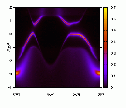
Figure 11: Single particle spectral density $A({\bf k},\omega)$ computed with the fitted self-energy (11) for the underdoped case $\delta=0.12$, the spectra are calculated with $\eta=0.05$.

We note first that the spectral density in Fig. 11 is in very good agreement with the spectral density obtained by Quantum Monte-Carlo (QMC) simulations of the underdoped Hubbard model, see e.g. Fig. 9 of Ref. Carsten . The two-band structure of the valence band, the flat high-intensity part around $(\pi,0)$ and the apparent nearest neighbor hopping band in the energy range $[-t:t]$ are completely consistent with QMC. The intensity of the upper band in the photoemission spectrum is low at $(0,0)$ and increases as the Fermi energy is approached, whereas the lower band at $-3t$ has a high intensity at $(0,0)$ and rapidly looses weight as is moves away from this momentum. This is in agreement with the QMC spectra as well.

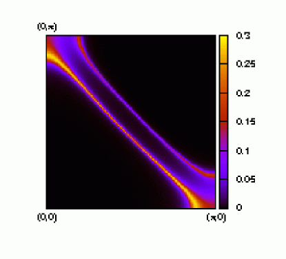
Figure 12: Single particle spectral density at $\mu$ computed with the fitted self-energy (11) for the underdoped case, $\delta=0.12$. The value of $\eta$ is $0.05$.

Figure 12 shows a Brillouin zone map of the spectral weight at $\mu$. The Fermi surface obviously takes the form of a ‘hole ring’ along the surface of the antiferromagnetic Brillouin zone. Since the free dispersion $\epsilon_{\bf k}$ is degenerate along the line $(\pi,0)\rightarrow(0,\pi)$ there is no hole pocket but a ‘hole ring’. Calculations for a single hole in the t-J model usually give - for moderate $J/t$ - a very small dispersion along this line and a shallow maximum at $(\frac{\pi}{2},\frac{\pi}{2})$Trugman ; Shraiman ; Inoue ; Ederbecker . If this band is filled with holes this results in hole pockets centered at $(\frac{\pi}{2},\frac{\pi}{2})$. The reason for the maximum is hole hopping along a spiral path as first discussed by TrugmanTrugman . The present calculation either misses this fine detail or it is not relevant in the doped system so that no maximum exists and the pockets are deformed into a ring. In any way, the Fermi surface clearly is ‘small’ in that it covers only a tiny fraction of the Brillouin zone. This is ultimately the consequence of the upward dispersing pole of $\Sigma({\bf k},\omega)$ near $(\pi,\pi)$. The fraction of the Brillouin zone covered by the ring is $17.3\%$. This is much larger than the value of $\delta/2=6\%$. The latter value would be obtained if the doped holes are modelled by spin-$1/2$ Fermions as suggested by exact diagonalizationlan and as predicted in a recent theory for lightly Mott insulatorsewo . It is quite obvious, however, that small changes in the parameters characterizing the fitted self energy may change this value strongly. The too large area of the ring thus probably simply shows the limited accuracy of the fit. One notable feature is the small spectral weight of the Fermi surface facing $(\pi,\pi)$ - this is very similar to the ‘remnant Fermi surface’.
Next, we consider the overdoped case and set $n=0.38$. Since there are no bands of poles close to $\mu$ and in particular the band of poles near $(\pi,\pi)$ is absent we expect a free-electron-like Fermi surface. This is indeed the case as can be seen from the Fermi surface map in Fig. 13. The fraction of the Brillouin zone covered by the large electron-like Fermi surface around $(0,0)$ is $0.382$, which is in very good agreement with the Luttinger theorem when the carriers are electrons. Taken together the data thus indicate a phase transition in between underdoping and overdoping from a phase with hole pockets - or a ‘hole ring’ in the present case - to one with a large Fermi surface.

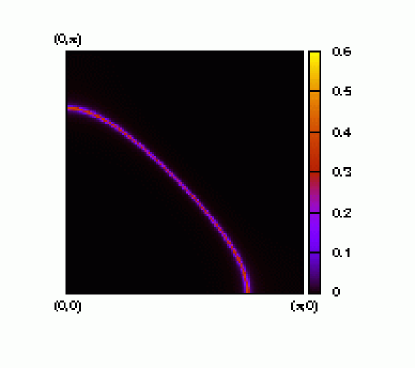
Figure 13: Single particle spectral density at $\mu$ computed with the fitted self-energy for the overdoped case.

V The self-energy in the underdoped regime

We have seen that a key feature of the underdoped system is the presence of an additional upward dispersing band of poles in $\Sigma({\bf k},\omega)$ near $(\pi,\pi)$, i.e. the band $\nu=2$. In the following we discuss some consequences of this band. We set

$$\epsilon_{\bf k}+\Sigma({\bf k},\omega+\mu)=\tilde{\epsilon}_{\bf k}+\frac{\sigma}{\omega-\zeta_{\bf k}}$$ (15)

where the first term on the r.h.s. is the sum of $\epsilon_{\bf k}$, $g_{\bf k}$ and the contribution from the other poles in $\Sigma({\bf k},\omega)$ and the second term represents the upward dispersing band $\nu=2$. We assume that $\tilde{\epsilon}_{\bf k}$ is a smooth function of ${\bf k}$ and for simplicity neglect its frequency dependence. In the absence of the isolated pole $\tilde{\epsilon}_{\bf k}$ therefore would be the quasiparticle dispersion. If additional poles of $\Sigma({\bf k},\omega)$ are sufficiently far away we obtain the two bands

$$\omega_{1,2}=\frac{1}{2}\left(\tilde{\epsilon}_{\bf k}+\zeta_{\bf k}\pm\sqrt{(\tilde{\epsilon}_{\bf k}-\zeta_{\bf k})^{2}+4\sigma}\right)$$ (16)

which are shown in Fig. 14. There is a gap of $2\sqrt{\sigma}$ between these bands. Far from the crossing point $\tilde{\epsilon}_{\bf k}=\zeta_{\bf k}$ the bands take the form

$$\omega_{1,2} = \tilde{\epsilon}_{\bf k}+\frac{\sigma}{\tilde{\epsilon}_{\bf k}-\zeta_{\bf k}}$$

$$\omega_{1,2} = \zeta_{\bf k}-\frac{\sigma}{\tilde{\epsilon}_{\bf k}-\zeta_{\bf k}}$$ (17)

The two resulting bands thus partially trace the quasiparticle band $\tilde{\epsilon}_{\bf k}$ and partially the dispersion of the pole, $\zeta_{\bf k}$. The spectral weight of the respective branches is

$$Z^{-1} = 1-\frac{\partial\tilde{\epsilon}_{\bf k}}{\partial\omega}+\frac{\sigma}{(\tilde{\epsilon}_{\bf k}-\zeta_{\bf k})^{2}}$$

$$Z^{-1} = 1-\frac{\partial\tilde{\epsilon}_{\bf k}}{\partial\omega}+\frac{(\tilde{\epsilon}_{\bf k}-\zeta_{\bf k})^{2}}{\sigma}$$ (18)

where the upper (lower) line refers to the band portion tracing $\tilde{\epsilon}_{\bf k}$ ($\zeta_{\bf k}$). Since far from the crossing point $(\tilde{\epsilon}_{\bf k}-\zeta_{\bf k})^{2}\gg\sigma$ the spectral weight $Z$ assumes its usual value for the band portion tracing $\tilde{\epsilon}_{\bf k}$ but is $\frac{\sigma}{(\tilde{\epsilon}_{\bf k}-\zeta_{\bf k})^{2}}\ll 1$ for the band portion tracing $\zeta_{\bf k}$. This behaviour can be seen along $(0,0)\rightarrow(\pi,\pi)$ and along $(\pi,0)\rightarrow(\pi,\pi)$ in Fig. 11. The upward dispersing band of poles in $\Sigma({\bf k},\omega)$ also has a major significance for the validity of the Luttinger theoremLuttingertheorem . To see this we derive a slightly modified version of the theorem which allows for an appealing physical interpretation. We consider

$$S = \frac{1}{2\pi i}\sum_{\bf k}\;\int_{C}\;d\omega\;G({\bf k},\omega)\;\frac{\partial\Sigma({\bf k},\omega)}{\partial\omega}$$

$$= \frac{1}{2\pi i}\sum_{\bf k}\;\int_{C}\;d\omega\;\left(\;G({\bf k},\omega)+\frac{1}{G({\bf k},\omega)}\;\frac{\partial G({\bf k},\omega)}{\partial\omega}\;\right)$$

where $C$ is a curve in the complex $\omega$-plane which encloses the part of the real axis with $\omega<\mu$ in counterclockwise fashion. All singularities of the integrand are located on the real axis. The first term in the second line will give the total electron number/spin. The second term has two kinds of singularties: poles and zeros of $G({\bf k},\omega)$. Near a pole we have

$$\frac{1}{G({\bf k},\omega)}\;\frac{\partial G({\bf k},\omega)}{\partial\omega} \approx \frac{-\frac{Z_{{\bf k},\nu}}{(\omega-\omega_{{\bf k},\nu})^{2}}}{\frac{Z_{{\bf k},\nu}}{(\omega-\omega_{{\bf k},\nu})}}+\dots$$

$$=-\frac{1}{(\omega-\omega_{{\bf k},\nu})}+\dots$$ (20)

whereas near a zero we have

$$\frac{1}{G({\bf k},\omega)}\;\frac{\partial G({\bf k},\omega)}{\partial\omega} \approx \frac{\sigma_{{\bf k},j}}{\sigma_{{\bf k},j}(\omega-\zeta_{{\bf k},j})}+\dots$$

$$=\frac{1}{(\omega-\zeta_{{\bf k},j})}+\dots$$ (21)

It follows that

$$N_{e} = 2S+2\sum_{\bf k}m_{\bf k}$$

$$m_{\bf k} = \sum_{\nu}\Theta(\mu-\omega_{{\bf k},\nu})-\sum_{j}\Theta(\mu-\zeta_{{\bf k},j}).$$ (22)

If we assume that $S=0$ we find that the number of electrons can be obtained by computing the number of ‘occupied’ poles of the Green’s function and subtracting the number of ‘occupied’ poles of the self-energy. A band of poles of the self-energy which crosses $\mu$ - such as the band $\nu=2$ introduced in the fit of the self-energy in the preceeding section - therefore produces a ‘negative volume Fermi surface’ because the number of momenta within this surface has to be subtracted in the computation of the electron number.
To arrive at the known form of the theorem we note that - as discussed in section II - there is exactly one pole of $G({\bf k},\omega)$ between any two successive poles of $\Sigma({\bf k},\omega)$. Moreover it is easy to see that there is always precisely one pole of $G({\bf k},\omega)$ below the lowest pole of $\Sigma({\bf k},\omega)$. Accordingly $m_{\bf k}=0$ if the topmost singularity below $\mu$ is a pole of the self-energy for the respective ${\bf k}$-point and $m_{\bf k}=1$ if the topmost singularity is a pole of the Green’s function. Since in the first case $\Re\;G({\bf k},\mu)<0$ whereas in the second case $\Re\;G({\bf k},\mu)>0$ we obtain

$$N_{e}=2\sum_{\bf k}\Theta(\Re\;G({\bf k},\mu))$$ (23)

which is the ‘generalized’ Luttinger theorem given by DzyaloshinskiiDzyalo . The equivalence of (22) and (23) has previously been noted by Ortloff et al.Ortloff .

Figure 14: Bare dispersion $\tilde{\epsilon}_{\bf k}$ intersecting with a band of poles of the self-energy, $\zeta_{\bf k}$.

It is then easy to see that - contrary to widespread belief - hole pockets can in fact be completely consistent with the Luttinger theorem. We again consider Fig. 14 which shows a situation where the dispersion $\tilde{\epsilon}_{\bf k}$ is intersected by an upward dispersing band of poles of the self-energy, $\zeta_{\bf k}$, resulting in the two quasiparticle bands $\omega_{1,{\bf k}}$ and $\omega_{2,{\bf k}}$. The lower of these bands, $\omega_{1,{\bf k}}$, crosses the Fermi energy - indicated by the horizontal dashed line - and produces two Fermi level crossings at the points $1$ and $2$ which form the hole pocket. In between $(0,0)\rightarrow 1$ we have $m_{\bf k}=1$ because the topmost pole below $\mu$ is the pole $\omega_{1,{\bf k}}$ of the Greens function. Along $1\rightarrow 2$ $m_{\bf k}=0$ because no pole of either Green’s function nor self-energy is below $\mu$. Additional singularities at lower energies do not change this: since the topmost singularity below $\omega_{1,{\bf k}}$ must be a pole of the self-energy, the total contribution to $m_{\bf k}$ from all singularities including this one is zero. Along the short piece $2\rightarrow 3$ we have again $m_{\bf k}=1$ but along $3\rightarrow(\pi,\pi)$ we have $m_{\bf k}=0$ because the topmost pole below $\mu$ now is one of the self-energy, $\zeta_{\bf k}$. The piece $2\rightarrow 3$ will be very short if the residuum $\sigma$ is small. The piece $3\rightarrow(\pi,\pi)$ corresponds precisely to the ‘negative volume Fermi surface’ discussed above because here the topmost singularity is a pole of the self-energy. Assuming that the total volume of the hole pockets is $V_{BZ}\;\delta/2$ - as suggested by a recent theory of the lightly doped Mott insulatorewo - the fraction of the Brillouin zone outside the pockets is $V_{BZ}\;(1-\delta/2)$. Then, if the ‘negative volume Fermi surface’ is $V_{BZ}/2$ the occupied part of the Brillouin zone in the sense of the Luttinger theorem would be $V_{BZ}(1-\delta)/2)$, i.e. corresponding precisely to the electron density. Hole pockets therefore would be completely consistent with the Luttinger theorem if this is applied correctly. For example, evaluation of (23) with the fitted self-energy for two holes - where the Fermi surface takes the form of a hole ring, see Fig. 12 - gives $N_{e}=1.032N$ whereas the correct value would be $N_{e}=0.88N$. The deviation of $\approx 15\%$ shows the limited accuracy of the fitted self-energy, but is far smaller than the difference in Fermi surface volume.

VI Comparison to ARPES experiments

ARPES experiments on underdoped cuprate superconductors show a number of interesting features and the next point is a comparison of the extrapolated cluster spectra to these experiments. Here an important point is to introduce longer range hopping terms. More precisely, we introduce an additional hopping term which connects next-nearest (i.e. $(1,1)$-like) neighbors. We choose the matrix element for this term to be $t^{\prime}=-0.4t$. This value is somewhat large but we simultaneously omit a hopping term between $(2,0)$-like neighbors because this would lead to a strong increase in the number of three-site terms in the strong coupling Hamiltonian. We performed the calculation only for the $16$- and $18$-site cluster with two holes because introduction of this additional hopping term increases the number of possible three-site combinations in the Hamiltonian considerably, so that the calculations become too difficult for the $20$-site cluster with two holes and the $18$-site cluster with $4$ holes. It turns out that the ground states of the two clusters with the $t^{\prime}$-term in the Hamiltonian have somewhat unusual quantum numbers: the ground state of two holes in the $16$-site cluster has momentum $(\pi,0)$ and spin $S=0$, the ground state of the $18$-site cluster with two holes has momentum $(\frac{2\pi}{3},0)$ and spin $S=1$. This means that the GS of the $16$-site cluster is twofold, that of the $18$-site cluster $12$-fold degenerate. This presents no real problem in that the expression (3) should be viewed as the zero temperature limit of a grand canonical average, so that in the case of GS-degeneracy one simply has to average over all degenerate ground states.

Figure 15: Spectral density $A({\bf k},\omega)$ and imaginary part of the self-energy $\Sigma({\bf k},\omega)$ for the $16$-site and $18$-site cluster with $2$ holes. The value $t^{\prime}=-0.4t$. The spectra are calculated with $\eta=0.05$ and $\Sigma({\bf k},\omega)$ is multiplied by 1/5.

From Fig. 4 and Table 1 it can be seen that the dispersion of the central pole within the gap $(\nu=1)$ is changed somewhat by the presence of $t^{\prime}$. In particular the deviations from the inverted nearest-neighbor-hopping dispersion become stronger. Figure 15 shows the single particle spectrum and self-energy in the presence of the $t^{\prime}$-term. By comparison with Fig. 5 it is obvious that the $t^{\prime}$-term introduces several pronounced changes in $\Sigma({\bf k},\omega)$: The residuum of the pole near $(\pi,\pi)$ ($\nu=2$) has decreased considerably, in fact this pole cannot seen anymore but takes the form of broad humps at the top of the incoherent continua, whose upper edge has moved closer to $\mu$. Instead there are now poles with large residuum at $(\pi,0)$ and $(\pi,\frac{\pi}{3})$. And finally there is no more pole at the top of the incoherent continuum and the intensity of the incoherent continua themselves has increased. To fit the self-energy we use the same ansatz (11) but drop the pole $\nu=3$ at the top of the incoherent continuum. The second difference concerns the strong pole near $(\pi,0)$. We assume that this pole actually belongs to the band $\nu=2$ and to model this we change the residuum of this band of poles by adding a second term:

$$\sigma_{{\bf k},2} = \sigma_{0}\;e^{-f({\bf k})/\alpha}+\sigma_{d}\;e^{\gamma_{d}^{2}/\beta^{2}}\;\gamma_{d}^{2}({\bf k}),$$

$$\gamma_{d}({\bf k}) = \cos(k_{x})-\cos(k_{y}).$$ (24)

The dispersion of this pole is again expanded with respect to only two harmonics, the constant $\gamma_{0}({\bf k})$ and the nearest-neighbor-hopping harmonic $\gamma_{1}({\bf k})$. As already mentioned the poles near $(\pi,\pi)$ cannot really be resolved in the calculated self-energies. Our main justification for keeping this band is the behaviour seen for $t^{\prime}=0$.

	$\zeta_{0,\nu}$	$\zeta_{1,\nu}$	$\sigma_{0}$	$\alpha$	$\sigma_{d}$	$\beta$
$\nu=2$	0.143	0.325	0.400	6.8	0.0184	1.15
	$\epsilon_{min}$	$\epsilon_{max}$	$\sigma_{c,0}$	$\sigma_{c,1}$
	-5.0	-0.5	0.25	0.5
	0.5	3.0	0.020	0.4
	7.0	12.0	0.025	1.0

Table 3: Coefficients of the model self-energy for $U/t=10$, $\delta\approx 10\%$, $t^{\prime}/t=-0.4$. The constant term $\zeta_{0,2}$ and the edges of the continua are relative to $\mu$. A comparison of the model self-energy and the numerical spectrum can be seen in Fig. 13.

Table 3 then gives the respective coefficients and Fig. 13 compares the numerical self-energy and the fit. The coefficient of $\gamma_{1}({\bf k})$ is positive. If only the term $\propto\sigma_{d}$ were kept in (24) the exponential $e^{\gamma_{d}^{2}/\alpha_{2}^{2}}$ replaced by unity and $\zeta_{0,\nu}$ be set to zero in this term, the resulting self-energy would be identical to the phenomenological self-energy introduced by Yang et al.YangRiceZhang . On the other hand the residuum clearly has an extremely strong ${\bf k}$-dependence so that the exponential cannot be neglected in the present fit.

Figure 16: Imaginary part of the self-energy $\Sigma({\bf k},\omega)$ for the $16$-site and $18$-site cluster with $2$ holes and Fit. The value $t^{\prime}=-0.4t$.

Figure 17 then shows the single particle spectral density obtained with the fitted self-energy. Along $(0,0)\rightarrow(\pi,\pi)$ the quasiparticle band disperses towards the Fermi energy. Consistent with experiment, the intensity of the band thereby increases as $\mu$ is approached.

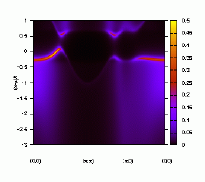
Figure 17: Single particle spectral density $A({\bf k},\omega)$ for $\delta=0.12$, $U/t=10$ and $t^{\prime}/t=-0.4$ obtained by using the interpolated self-energy for the infinite lattice.

After crossing $\mu$ the band turns downward sharply and immediately crosses $\mu$ again whereby its spectral weight drops. This is precisely the situation shown in Fig. 14. Along $(0,0)\rightarrow(\pi,0)$ the band disperses upward as well but does not reach $\mu$. The ARPES spectrum thus shows a ‘pseudogap’ but this is a trivial consequence of the Fermi surface being a hole pocket centered at $(\frac{\pi}{2},\frac{\pi}{2})$ (see below). Roughly at $(\frac{4\pi}{5},0)$ there is a maximum of the dispersion with high spectral weight and the band turns downward and looses weight beyond this point. This behaviour may actually have been observed by Chuang et al.Chuang who interpreted this as indicating a Fermi level crossing at $\approx(\frac{4\pi}{5},0)$. Chuang et al. observed this behaviour in an underdoped compound - see Fig. 2i of Ref. Chuang - but also in overdoped samples where it is unclear if it can be compared to the present calculation. In contrast the spectral weight around $(\pi,0)$ is small. This is consistent with experiment where a quasiparticle band around $(\pi,0)$ is usually not observed in the normal state of underdoped cuprate superconductors. Along the line $(\pi,0)\rightarrow(\pi,\pi)$ the band seems to disperse upward at first, but then again bends sharply and disperses away from $\mu$. At the turning point the spectral weight drops. This is again due to the avoided crossing of the quasiparticle band with the upward dispersing band of poles of $\Sigma({\bf k},\omega)$ near $(\pi,\pi)$, i.e. the band $\nu=2$, in Fig. 14. A very similar behaviour has in fact been observed experimentally in underdoped La_2-xSr_xCuO₄, see Fig. 5 of Ref. Ino . In this compound the quasiparticle band is sufficiently far from $\mu$ at $(\pi,0)$ so that the absence of a Fermi level crossing is obvious for $x=0.05$ and $x=0.10$. A very avoided crossing has been observed as ‘backbending’ of bands in Bi2201 in Ref. Hashimoto . If such an avoided crossing would occur sufficiently close to $\mu$, however, it may look very similar to a true Fermi level crossing. Aparent experimental Fermi level crossings along $(\pi,0)\rightarrow(\pi,\pi)$ thus should be considered with care.
The actual Fermi surface of the underdoped system is shown in Fig. 18 and takes the form of a hole pocket, centered near $(\frac{\pi}{2},\frac{\pi}{2})$. The pocket is shifted slightly towards $(0,0)$ and the part facing $(\pi,\pi)$ has smaller spectral weight and less curvature than the part facing $(0,0)$. The pockets covers $1.86\%$ of the total Brillouin zone which would correspond - assuming twofold spin degeneracy and four equaivalent pockets - to a quasiparticle density of $14.9\%$. This is close to the hole concentration of $12\%$. On the other hand the electron density as computed from the Luttinger theorem (23) is $1.25$ so that the inaccuracies of the self energy clearly are substabtial and the close agreement for the quasiparticle density may be fortuitious.

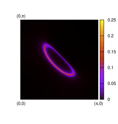
Figure 18: Single particle spectral density at $\mu$ for $\delta=0.12$, $U/t=10$ and $t^{\prime}/t=-0.4$ obtained by using the interpolated self-energy for the infinite lattice.

VII Discussion

In summary we have presented an exact diagonalization study of the self-energy $\Sigma({\bf k},\omega)$ in the 2D Hubbard model. Larger clusters than usual could be used because instead of studying the true Hubbard model we considered its strong-coupling limit which requires much smaller Hilbert spaces. For dopings less than 30% - i.e. the doping region in which cuprate superconductivity takes place - several distinct features can be identified: first, a pole with large residuum $\propto(U/t)^{2}$ and a dispersion of width $\propto t$ in the center of the Hubbard gap, which is present throughout this doping range. Second, a pole with smaller residuum and an upward dispersion $\propto J$ around $(\pi,\pi)$ which is present only in the underdoped regime. And third, several broad incoherent continua of width $\propto t$. The top of the lowest of these incoherent continua may be formed by a third pole. All features in the spectral representation of $\Sigma({\bf k},\omega)$ show a pronounced ${\bf k}$-dependence, both with respect to their dispersion and their residuum. This implies that in real space the self-energy is long-ranged and oscillatory.
The key difference between the underdoped and overdoped system is the presence of a dispersive pole of $\Sigma({\bf k},\omega)$ around $(\pi,\pi)$. This pole cuts through the quasiparticle dispersion and changes the Fermi surface topology completely. In the underdoped hole concentration range the Fermi surface takes the form of a ‘hole ring’ for $t^{\prime}=0$ or hole pockets centered near $(\frac{\pi}{2},\frac{\pi}{2})$ for $t^{\prime}=-0.4t$ and changes to a large free-electron-like Fermi surface in the overdoped case. We have shown that the hole pockets can be completely consistent with the Luttinger theorem. The residuum of the upward dispersing pole near $(\pi,\pi)$ thus plays the role of an order parameter for the phase transition between the two different ground states.
The single-particle spectra obtained with the fitted self-energies agree very well with both Quantum Monte Carlo simulations (for $t^{\prime}=0$) and ARPES on underdoped cuprates (for $t^{\prime}=0.4t$). In particular the spectra reproduce a hole-pocket-like Fermi surface of similar shape and location as in experiment and also the characteristic strong asymmetry of the spectral weight of the parts of the pocket facing $(0,0)$ and $(\pi,\pi)$. Quite generally, the spectra show that all parts of the quasiparticle band which deviate from the noninteracting electron band structure have a very small weight. The reason is that these band portions closely follow the dispersion of a band of poles of $\Sigma({\bf k},\omega)$ and ‘borrow’ their spectral weight from the quasiparticle band. The data suggest in particular that some Fermi level crossings observed in ARPES along the line $(\pi,0)\rightarrow(\pi,\pi)$ actually may not be true Fermi level crossings but sharp bends at the intersection of the quasiparticle dispersion and a band of poles in $\Sigma({\bf k},\omega)$. An example where such pseudo-crossings can be clearly recognized is La_2-xSr_xCuO₄Ino . In this compound the shift the quasiparticle band is sufficiently far from $\mu$ near $(\pi,0)$ so that the absence of a Fermi level crossing is clear - if the quasiparticle band is closer to $\mu$, however, there pseudo-crossing may well be mistaken for a real Fermi level crossing.
An interesting question is the physical meaning of the upwards dispersing pole near $(\pi,\pi)$. One immediate consequence of this pole is that the part of the inverse photoemission spectrum belonging to the lower Hubbard band consists of two disconneted components. The first component is the unoccupied part of the quasiparticle band, which forms the cap of the hole-pockets around $(\frac{\pi}{2},\frac{\pi}{2})$, the second component is a disconnected part around $(\pi,\pi)$. This two-component nature of the inverse phtoemission spectrum was discussed in Ref. inverse where it was shown that the disconnected component around $(\pi,\pi)$ actually consists of spin-polaron shakeoff, i.e. spin excitations which are released when a hole dressed by antiferromagnetic spin fluctuations is filled by an electron. The disconnected nature of the low energy inverse photoemission spectrum thus is a quite natural consequence of the hole pockets and the spin-polaron nature of the quasiparticles.
The transition then may be understood as follows: in a Mott insulator the electrons are localized and retain only their spin degrees of freedom. Upon doping most electrons are still tightly surrounded by other electrons as in the insulator and thus remain localized - the ground state wave function therefore should optimize the energy gain due to delocalization of the holes and since the holes are spin-1/2 Fermions this can be achieved by forming hole pockets with a volume $\propto\delta$ around the ground state momentum of a single hole i.e. $(\frac{\pi}{2},\frac{\pi}{2})$. This picture leads to a simple theoryewo in which the number of noninteracting particles is equal to the number of doped holes.
When the density of holes becomes sufficiently large so that the electrons are sufficiently mobile a phase transition occurs to a state which optimizes the kinetic energy of the electrons themselves and this means the formation of a Fermi surface with a volume $\propto 1-\delta$. A rough estimate for the hole concentration where the transition occurs would be $\delta_{c}\approx z^{-1}$ with $z$ the coordination number because then each electron has one unoccupied neighbor on the average. The vanishing of the upward dispersing pole in the self-energy then corresponds to this phase transition. Experimentally it seems that the phase transition between pockets and free-electron-like Fermi surface occurs right at optimal doping. This suggests that superconductivity is also related to this transition.
Acknowledgement: K. S. acknowledges the JSPS Re- search Fellowships for Young Scientists. R. E. most gratefully acknowledges the kind hospitality at the Cen- ter for Frontier Science, Chiba University. This work was supported in part by a Grant-in-Aid for Scientific Research (Grant No. 22540363) From the Ministry of Education, Culture, Sports, Science and Technology of Japan. A part of the computations was carried out at the Research Center for Computational Science, Okazaki Re- search Facilities and the Institute for Solid State Physics, University of Tokyo.

VIII Appendix A

Here we proove that the real constant $g_{\bf k}$ in (2) is equal to the Hartree-Fock potential. Considering the limit of large $\omega$, expanding the two expressions for the Green’s function, (2) and (3), in powers of $\omega^{-1}$ thereby using (4) one obtains by comparing the terms $\propto\omega^{-2}$:

$$\epsilon_{\bf k}+g_{\bf k}=\langle\Psi_{0}|\left[c_{{\bf k},\sigma}[H,c_{{\bf k},\sigma}^{\dagger}]\right]_{+}|\Psi_{0}\rangle$$ (25)

where $[\dots]_{+}$ denotes the anticommutator. Using a standard Hamiltonian of the form

$$H = \sum_{{\bf k},\sigma}\epsilon_{\bf k}c_{{\bf k},\sigma}^{\dagger}c_{{\bf k},\sigma}$$

$$+ \frac{1}{2}\sum_{{\bf k},{\bf k}^{\prime},{\bf q}}\sum_{\sigma,\sigma^{\prime}}V_{{\bf k}+{\bf q},{\bf k},{\bf k}^{\prime}-{\bf q},{\bf k}^{\prime}}^{\sigma\sigma^{\prime}}c_{{\bf k}+{\bf q},\sigma}^{\dagger}c_{{\bf k}^{\prime}-{\bf q},\sigma^{\prime}}^{\dagger}c_{{\bf k}^{\prime},\sigma^{\prime}}c_{{\bf k},\sigma}$$

this gives

$$g_{\bf k}=\sum_{{\bf k}^{\prime},\sigma^{\prime}}V_{{\bf k},{\bf k}^{\prime},{\bf k}^{\prime},{\bf k}}^{\sigma,\sigma^{\prime}}\langle n_{{\bf k}^{\prime},\sigma^{\prime}}\rangle-\sum_{{\bf k}^{\prime}}V_{{\bf k},{\bf k}^{\prime},{\bf k},{\bf k}^{\prime}}^{\sigma,\sigma}\langle n_{{\bf k}^{\prime},\sigma}\rangle.$$ (26)

where $\langle\dots\rangle$ denotes the ground state expectation value.

IX Appendix B

The canonical transformation which reduces the full Hubbard Hamiltonian to the strong-coupling Hamiltonian takes the form

$$O^{\prime}=e^{S}Oe^{-S}$$ (27)

where $O$ denotes an operator in the original Hilbert space and $O^{\prime}$ is the transformed operator. The antihermitean generator $S$ is

$$S = -\sum_{i,j}\sum_{\sigma}\;\frac{t_{ij}}{U}\;\left(\hat{d}_{i,\sigma}^{\dagger}\hat{c}_{j,\sigma}-\hat{c}_{i,\sigma}^{\dagger}\hat{d}_{i,\sigma}\right)$$

$$\hat{d}_{i,\sigma}^{\dagger} = c_{i,\sigma}^{\dagger}n_{i,\bar{\sigma}}$$

$$\hat{c}_{i,\sigma}^{\dagger} = c_{i,\sigma}^{\dagger}(1-n_{i,\bar{\sigma}}).$$ (28)

The strong-coupling Hamitonian or corrected t-J model is obtained by transforming the Hubbard Hamiltonian according to (27) and discarding terms of 2^nd or higher order in $1/U$. The complete - and somewhat lengthy - Hamiltonian in given in equation (14) of the paper by Eskes et al.Eskesetal . The transformed version of the electron annihilation operator is

$$e^{S}c_{i,\uparrow}e^{-S} = c_{i,\uparrow}-\sum_{j}\frac{t_{ij}}{U}(\;\hat{d}_{j,\downarrow}^{\dagger}-\hat{c}_{j,\downarrow}^{\dagger})\;c_{i,\downarrow}c_{i,\uparrow}$$ (29)

$$+ (\hat{c}_{j,\downarrow}-\hat{d}_{j,\downarrow})\;S_{i}^{-}+n_{i,\downarrow}(2n_{i,\uparrow}-1)\hat{c}_{j,\uparrow}$$

$$- (1-n_{i,\downarrow})(2n_{i,\uparrow}-1)\hat{d}_{j,\uparrow}\;)$$

where again terms of higher order in $t/U$ have been neglected. By collecting the terms which give a nonvanishing result when acting on a state without double occupancies and do not produce a double occupancy themselves we obtain the operator for photoemission in the lower Hubbard bandEskesetal :

$$\tilde{c}_{i,\uparrow}=\hat{c}_{i,\uparrow}-\sum_{j}\;\frac{t_{ij}}{U}\;\left(\hat{c}_{j,\uparrow}n_{i,\downarrow}-\hat{c}_{j,\downarrow}S_{i}^{-}\right).$$ (30)

Since the transformed creation operator is the Hermitean conjugate of (29), the operator for inverse photoemission with final states in the lower Hubbard band is just the Hermitean conjugate of (30). The operator for inverse photoemission with final states in the upper Hubbard band is obtained by taking the Hermitean conjugate of (29) and collecting terms which create a double occupancy but do not annihilate one:

$$\tilde{c}_{i,\uparrow}^{\dagger} = \hat{d}_{i,\uparrow}+\sum_{j}\;\frac{t_{ij}}{U}\;(\;\;\hat{c}_{j,\downarrow}\;c_{i,\downarrow}^{\dagger}\;c_{i,\uparrow}^{\dagger}$$ (31)

$$+ \hat{d}_{j,\downarrow}^{\dagger}\;S_{i}^{+}+\hat{d}_{j,\uparrow}^{\dagger}\;(1-n_{i,\downarrow})(2n_{i,\uparrow}-1)\;).$$

References

- (1) N. E. Hussey, M. Abdel-Jawad, A. Carrington, A. P. Mackenzie, and L. Balicas, Nature 425, 814 (2003).
- (2) M. Plate, J. D. F. Mottershead, I. S. Elfimov, D. C. Peets, R. Liang, D. A. Bonn, W. N. Hardy, S. Chiuzbaian, M. Falub, M. Shi, L. Patthey, and A. Damascelli, Phys. Rev. Lett. 95, 077001 (2005).
- (3) B. Vignolle, A. Carrington, R. A. Cooper, M. M. J. French, A. P. Mackenzie, C. Jaudet, D. Vignolles, Cyril Proust, N. E. Hussey Nature 455, 952 (2008).
- (4) A. Damascelli, Z. Hussain, and Z.-X. Shen, Rev. Mod. Phys. 75, 473 (2003).
- (5) B. O. Wells, Z.-X. Shen, A. Matsuura, D. M. King, M. A. Kastner, M. Greven, and R. J. Birgeneau, Phys. Rev. Lett. 74, 964 (1995).
- (6) F. Ronning, C. Kim, D. L. Feng, D. S. Marshall, A. G. Loeser, L. L. Miller, J. N. Eckstein, L. Bozovic, and Z.-X. Shen, Science 282, 2067 (1998).
- (7) S. Uchida, T. Ido, H. Takagi, T. Arima, Y. Tokura, and S. Tajima Phys. Rev. B 43, 7942 (1991).
- (8) W. J. Padilla, Y. S. Lee, M. Dumm, G. Blumberg, S. Ono, K. Segawa, S. Komiya, Y. Ando, and D. N. Basov Phys. Rev. B 72, 060511 (2005).
- (9) N. P. Ong, Z. Z. Wang, J. Clayhold, J. M. Tarascon, L. H. Greene, and W. R. McKinnon Phys. Rev. B 35, 8807 (1987).
- (10) H. Takagi, T. Ido, S. Ishibashi, M. Uota, S. Uchida, and Y. Tokura, Phys. Rev. B 40, 2254 (1989).
- (11) Y. Ando, Y. Kurita, S. Komiya, S. Ono, and K. Segawa, Phys. Rev. Lett. 92, 197001 (2004).
- (12) N. Doiron-Leyraud, C. Proust, D. LeBoeuf, J. Levallois, J.-B. Bonnemaison, R. Liang, D.A. Bonn, W.N. Hardy, and L. Taillefer, Nature 447, 565 (2007).
- (13) S. E. Sebastian, N. Harrison, E. Palm, T. P. Murphy, C. H. Mielke, R. Liang, D. A. Bonn, W. N. Hardy, and G. G. Lonzarich, Nature 454, 200 (2008).
- (14) C. Jaudet, D. Vignolles, A. Audouard, J. Levallois, D. LeBoeuf, N. Doiron-Leyraud, B. Vignolle, M. Nardone, A. Zitouni, R. Liang, D. A. Bonn, W. N. Hardy, L. Taillefer, and C. Proust, Phys. Rev. Lett. 100, 187005 (2008).
- (15) A. Audouard, C. Jaudet, D. Vignolles, R. Liang, D. A. Bonn, W. N. Hardy, L. Taillefer, and C. Proust, Phys. Rev. Lett. 103, 157003 (2009).
- (16) E. A. Yelland , J. Singleton , C. H. Mielke , N. Harrison, F. F. Balakirev, B. Dabrowski , J. R. Cooper, Phys. Rev. Lett. 100, 047003 (2008).
- (17) A. F. Bangura, J. D. Fletcher, A. Carrington, J. Levallois, M. Nardone, B. Vignolle, P. J. Heard, N. Doiron-Leyraud, D. LeBoeuf, L. Taillefer, S. Adachi, C. Proust, and N. E. Hussey, Phys. Rev. Lett. 100, 047004 (2008).
- (18) D. LeBoeuf, N. Doiron-Leyraud, J. Levallois, R. Daou, J.-B. Bonnemaison, N. E. Hussey, L. Balicas, B. J. Ramshaw, R. Liang, D. A. Bonn, W. N. Hardy, S. Adachi, C. Proust, and L. Taillefer, Nature 450, 533 (2007).
- (19) J. Chang, R. Daou, Cyril Proust, David LeBoeuf, Nicolas Doiron-Leyraud, Francis Laliberte, B. Pingault, B. J. Ramshaw, Ruixing Liang, D. A. Bonn, W. N. Hardy, H. Takagi, A. B. Antunes, I. Sheikin, K. Behnia, and Louis Taillefer, Phys. Rev. Lett. 104, 057005 (2010).
- (20) V. Hinkov, B. Keimer, A. Ivanov, P. Bourges, Y. Sidis, and C. D. Frost, arXiv:1006.3278v1
- (21) M. J. Lawler, K. Fujita, Jhinhwan Lee, A.R. Schmidt, Y. Kohsaka, Chung Koo Kim, H. Eisaki, S. Uchida, J.C. Davis, J.P. Sethna, and Eun-Ah Kim Nature 466, 347, (2010).
- (22) R. Eder and Y. Ohta, Phys. Rev. B 51, 6041 (1995).
- (23) P. W. Leung, Phys. Rev. B 65, 205101 (2002).
- (24) P. W. Leung, Phys. Rev. B 73, 014502 (2006).
- (25) E. Dagotto and J. R. Schrieffer, Phys. Rev. B 43, 8705 (1991).
- (26) R. Eder, Y. Ohta, and T. Shimozato, Phys. Rev. B 50, 3350 (1994).
- (27) R. Eder and Y. Ohta, Phys. Rev. B 50, 10043 (1994).
- (28) S. Nishimoto, Y. Ohta, and R. Eder Phys. Rev. B 57, R5590 (1998).
- (29) T. Tohyama, P. Horsch, and S. Maekawa, Phys. Rev. Lett. 74, 980 (1995).
- (30) R. Eder, Y. Ohta, and S. Maekawa, Phys. Rev. Lett. 74, 5124 (1995).
- (31) R. Eder and Y. Ohta, Phys. Rev. B 51, 11683 (1995).
- (32) M. Vojta and K. W. Becker, Europhys. Lett. 38, 607 (1997).
- (33) J. M. Luttinger, Phys. Rev. 121, 942 (1961).
- (34) E. Dagotto, Rev. Mod. Phys. 66, 763 (1994).
- (35) J. Hubbard, Proc. Roy. Soc. London, Ser. A 277, 237 (1964), and 281, 401 (1964).
- (36) E. Dagotto, F. Ortolani, and D. Scalapino, Phys. Rev. B 46, 3183 (1992).
- (37) P. W. Leung, Z. Liu, E. Manousakis, M. A. Novotny, and P. E. Oppenheimer, Phys. Rev. B 46, 11779 (1992).
- (38) A.B. Harris and R.V. Lange, Phys. Rev. 157, 295 (1967).
- (39) K. A. Chao, J. Spalek and A. M. Oles, J. Phys. C 10, L271 (1977).
- (40) A. H. MacDonald, S. M. Girvin and D. Yoshioka, Phys. Rev. B 37, 9753 (1988).
- (41) H. Eskes, A. M. Oles, M. B. J. Meinders, and W. Stephan, Phys. Rev. B 50, 17980 (1994).
- (42) H. Eskes and A. M. Oles, Phys. Rev. Lett. 73, 1279 (1994).
- (43) H. Eskes and R. Eder, Phys. Rev. B 54, R14226 (1996).
- (44) T. D. Stanescu and G. Kotliar, Phys. Rev. B 74, 125110 (2006).
- (45) S. Sakai, Y. Motome, and M. Imada, Phys. Rev. Lett. 102, 056404, (2009).
- (46) S. Sakai, Y. Motome, and M. Imada, Phys. Rev. B 82, 134505 (2010).
- (47) R. Eder and Y. Ohta, Phys. Rev. B 54, 3576 (1996).
- (48) C. Gröber, R. Eder, and W. Hanke, Phys. Rev. B 62, 4336 (2000).
- (49) S. A. Trugman, Phys. Rev. B 37, 1597 (1988).
- (50) B. I. Shraiman and E. D. Siggia, Phys. Rev. Lett. 60, 740 (1988).
- (51) J. Inoue and S. Maekawa, J. Phys. Soc. Jpn. 59, 2110 (1989).
- (52) R. Eder and K. W. Becker, Z. Phys. B 78, 219 (1990).
- (53) R. Eder, P. Wrobel, and Y. Ohta, Phys. Rev. B 82, 155109 (2010).
- (54) J. M. Luttinger, Phys. Rev. xx,
- (55) I. Dzyaloshinskii, Phys. Rev. B 68, 085113 (2003).
- (56) J. Ortloff, M. Balzer, and M. Potthoff, Eur. Phys. J. B 58, 37 (2007).
- (57) K.-Y. Yang, T. M. Rice, and F.-C. Zhang, Phys. Rev. B 73, 174501 2006.
- (58) Y.-D. Chuang, A. D. Gromko, D. S. Dessau, Y. Aiura, Y. Yamaguchi, K. Oka, A. J. Arko, J. Joyce, H. Eisaki, S. I. Uchida, K. Nakamura, and Yoichi Ando, Phys. Rev. Lett. 83, 3717, (1999).
- (59) A. Ino, C. Kim, M. Nakamura, T. Yoshida, T. Mizokawa, A. Fujimori, Z.-X. Shen, T. Kakeshita, H. Eisaki, and S. Uchida, Phys. Rev. B 65, 094504 (2002).
- (60) M. Hashimoto, R.-H. He, K. Tanaka, J.-P. Testaud, W. Meevasana, R. G. Moore, D. Lu, H. Yao, Y. Yoshida, H. Eisaki, T. P. Deveraux, Z. Hussain, and Z.-X. Shen, Nature Physics 6, 414 (2010).