Competition between the Fulde-Ferrell-Larkin-Ovchinnikov phase and the BCS phase in the presence of an optical potential

Abstract

In three dimensional Fermi gases with spin imbalance, a competition exists between Cooper pairing with zero and with finite momentum. The latter gives rise to the Fulde-Ferrell-Larkin-Ovchinnikov (FFLO) superfluid phase, which only exists in a restricted area of the phase diagram as a function of chemical potential imbalance and interaction strength. Applying an optical potential along one direction enhances the FFLO region in this phase diagram. In this paper, we construct the phase diagram as a function of polarization and interaction strength in order to study the competition between the FFLO phase and the spin balanced BCS phase. This allows to take into account the region of phase separation, and provides a more direct connection with experiment. Subsequently, we investigate the effects of the wavelength and the depth of the optical potential, which is applied along one direction, on the FFLO state. It is shown that the FFLO state can exist up to a higher level of spin imbalance if the wavelength of the optical potential becomes smaller. Our results give rise to an interesting effect: the maximal polarization at which the FFLO state can exist, decreases when the interaction strength exceeds a certain critical value. This counterintuitive phenomenon is discussed and the connection to the optical potential is explained.

I Introduction

In the past decennium, the field of cold atoms has witnessed the experimental realization of various new quantum coherent phenomena in ultracold gases Review Dalibard . Amongst the various systems that are being studied, fermionic superfluids occupy a prominent role Greiner ; Chin ; Zwierlein Ketterle . Contrary to bosonic gases, fermionic gases must form pairs between fermions in different spin states in order to form an s-wave superfluid. A fundamental question that has attracted wide attention recently, is what happens when the ratio between these different spin-states is altered, thereby creating a spin-imbalanced or polarized superfluid. This effect is akin to applying a magnetic field to a superconductor, which leads to electrons aligning their spins. In superconductors, and in condensed matter systems in general, it is difficult to control various parameters such as the polarization or the interaction strength. In ultracold gases, however, one has an unprecedented degree of control over these parameters Bloch review ; Greiner Q and A . For instance, experimentalists can tune the interaction strength by making use of Feshbach resonances (for a review on this subject see Ref. Chin Grimm ). Using this technique, the crossover from a Bardeen-Cooper-Schrieffer (BCS) superfluid to a Bose-Einstein condensate (BEC) of bound molecules has been studied Regal Greiner ; Bourdel Salomon ; Partridge Hulet ; De Melo . Furthermore, polarization can be created by first loading particles into one hyperfine state and subsequently applying a radio-frequency sweep to send a controlled number of particles to a different hyperfine state. This experimental liberty has led to the realization of many experiments on the imbalanced ultracold Fermi gas Zwierlein Ketterle 2 ; Shin Ketterle ; Partridge Hulet 2 ; Hulet en Stoof ; Schunck . Today, the main phases of this system, as a function of temperature, interaction strength and polarization, have been observed experimentally Ketterle FD . One of the most fundamental effects that occurs in a polarized Fermi gas is that above a critical imbalance, fermionic superfluidity ceases to exist and the system makes a transition into a normal Fermi gas. This is known as the Clogston-Chandrasekhar limit Clogston-Chandrasekhar . One important question that has emerged is whether there exist other pairing-mechanisms by which a gas of interacting fermions can accommodate polarized superfluidity. Recently, there has been an intensive theoretical search for these exotic superfluid phases, such as the breached pair or Sarma phase Sarma ; Sarma Studies , and phase separation Phase separation . Another phase that has attracted wide attention is the Fulde-Ferrell-Larkin-Ovchinnikov phase (FFLO phase), that was proposed independently by Fulde and Ferrell Fulde Ferell and by Larkin and Ovchinnikov Larkin Ovchinnikov in 1964. Their idea was that a fermionic system can accommodate spin imbalance, by forming pairs with finite center-of-mass momentum. Up till now, this state has never been observed. A recent paper reports indirect experimental evidence for the FFLO state in one dimension (1D) Liao Rittner , but in three dimensions (3D), the FFLO state has so far eluded experimental observation. This can be related to theoretical predictions, which state that the FFLO state only occupies a tiny sliver of the BCS-BEC crossover phase diagram Hu Liu ; Sheehy Radzihovsky . It was therefore necessary to find a new method to stabilize the FFLO state in 3D. At the moment, new ideas are emerging to realize this goal. For instance, in two recent papers, it was suggested to stabilize the FFLO state by the use of a 3D cubic lattice Koponen ; Trivedi . As an alternative approach, we proposed to stabilize the FFLO state in an imbalanced 3D Fermi gas by adding a 1D optical potential to this system Devreese Klimin en Tempere (2011) . This turned out to enhance the stability region of the FFLO state by up to a factor six. In Ref. Devreese Klimin en Tempere (2011) , the proof of principle for this concept was established using the path integral method , but questions remained about the exact effects of the properties of the optical potential on the FFLO state. In this paper, we investigate the role of the optical potential in detail. Our aim here is to present results that relate closely to the experiment. To this end, we construct and discuss the phase diagrams of an imbalanced Fermi gas in 3D, subjected to a 1D optical potential, both at fixed chemical potentials and at fixed densities. Subsequently, we investigate and discuss the effects of the properties of the optical potential on the BCS superfluid state and on the FFLO state. In Sec. II we outline our strategy to construct the phase diagrams at fixed chemical potentials and at fixed densities. Subsequently, we discuss the competition between the BCS phase and the FFLO phase in these phase diagrams, which differ qualitatively from the corresponding phase diagrams for the imbalanced Fermi gas in 3D without the optical potential. In Sec. III, we investigate the effects of the parameters of the optical potential on the FFLO state. Furthermore, we explain the remarkable effect that the maximal polarization at which the FFLO state can exist decreases when the interaction strength is increased above a certain critical value. Finally in section IV we draw conclusions.

II Construction of the phase diagrams

II.1 Phase diagram at fixed chemical potentials

To construct the phase diagram of an imbalanced 3D Fermi gas, subjected to a 1D optical potential, at fixed chemical potentials, we start from the saddle-point free energy per unit volume of this system, which is given by Devreese Klimin en Tempere (2011) :

$$\Omega_{sp}\left(\mu,\zeta;\Delta,Q\right) =-\frac{1}{\left(2\pi\right)^{2}}\int_{0}^{+\infty}dk~{}k~{}\int_{-Q_{L}}^{+Q_{L}}dk_{z}$$

$$\times\left[\max\left[\left|\zeta_{k,Q}\right|,E_{\mathbf{k}}\right]-\xi_{\mathbf{k}}-\frac{\Delta^{2}}{2\left\{k^{2}+\delta\left[1-\cos\left(\frac{\pi k_{z}}{Q_{L}}\right)\right]\right\}}\right]+\frac{\Delta^{2}}{8\pi}$$ (1)

with

$$\left\{\begin{array}[c]{l}\xi_{\mathbf{k}}=k^{2}+\delta\left[1-\cos\left(\frac{\pi}{2}\frac{Q}{Q_{L}}\right)\cos\left(\frac{\pi k_{z}}{Q_{L}}\right)\right]-\mu\\ E_{\mathbf{k}}=\sqrt{\xi_{\mathbf{k}}^{2}+\Delta^{2}}\\ \zeta_{k,Q}=\zeta-\delta\sin\left(\frac{\pi}{2}\frac{Q}{Q_{L}}\right)\sin\left(\frac{\pi k_{z}}{Q_{L}}\right)\end{array}\right..$$ (2)

To derive expression (1), the 1D optical potential was described by using a modified dispersion relation for the fermionic particles:

$$\varepsilon(k,k_{z})=k^{2}+\delta\left[1-\cos\left(\frac{\pi k_{z}}{Q_{L}}\right)\right],$$ (3)

where $\delta$ is a function of the depth of the potential $V_{0}$ and of the recoil energy $E_{R}$, and $Q_{L}$ is the wave vector of the optical potential. Expression (3) consists of a free particle dispersion in the directions perpendicular to the optical potential, and a tight-binding periodic dispersion Menotti in the direction parallel to the optical potential. Because we want to describe the FFLO state, we only consider the BCS-side of the BCS-BEC crossover Iskin de Melo ; Radzihovsky . In this region, the scattering length is always negative, hence the following units are used (1): $\hbar=2m=-a_{s}=1$, where $a_{s}$ is the s-wave scattering length. Here it must be mentioned that the derivation leading to the free energy (1) neglected the density modulation of the Fermi gas due to the 1D optical potential. This approximation leads to an underestimation of the interactions between the spin-up and spin-down fermions.

The free energy (1) depends on two thermodynamic variables $\mu$ and $\zeta$, and on two variational parameters $\Delta$ en $Q$. The variables $\mu$ and $\zeta$ are the total chemical potential $\mu=\left(\mu_{\uparrow}+\mu_{\downarrow}\right)/2$, which fixes the total density, and the imbalance chemical potential $\zeta=\left(\mu_{\uparrow}-\mu_{\downarrow}\right)/2$, which fixes the polarization. A description in terms of $\mu$ and $\zeta$ is equivalent to a description in terms of the respective chemical potentials of both spin species $\mu_{\uparrow}$ and $\mu_{\downarrow}$. The variational parameters $\Delta$ and $Q$ denote the binding energy and the center-of-mass momentum of the fermion pairs respectively. The parameter $Q$ was introduced to include the FFLO state (which is characterized by fermion pairs with finite momentum) in our description. To find the ground state of the system, given fixed values of $\mu$ and $\zeta$, the saddle-point free energy $\Omega_{sp}\left(\mu,\zeta;\Delta,Q\right)$ has to be minimized with respect to the variational parameters $\Delta$ and $Q$. This defines the saddle-point equations

$$\left\{\begin{array}[c]{c}\left.\dfrac{\partial\Omega_{sp}\left(\mu,\zeta;\Delta,Q\right)}{\partial\Delta}\right|_{\mu,\zeta}=0\\ \left.\dfrac{\partial\Omega_{sp}\left(\mu,\zeta;\Delta,Q\right)}{\partial Q}\right|_{\mu,\zeta}=0\end{array}\right.,$$ (4)

which have to be satisfied simultaneously. One must be careful when extremizing the free energy, because only the minima correspond to a stable physical state. We avoided this difficulty by explicitly minimizing the free energy, instead of searching for roots of (4). Depending on the values of the parameters $\mu$ and $\zeta$, three different ground states can emerge: 1) a spin-balanced (S-b) superfluid, with $\Delta\neq 0$ and $Q=0$ , 2) the FFLO state with $\Delta\neq 0$ and $Q\neq 0$, and 3) the normal state with $\Delta=0$. Moreover, in the phase diagrams we will make a distinction between the partially polarized normal state (PPN) and the fully polarized normal state (FPN). In the latter, all particles are in the same spin-state, while in the former both spin-states are still present. Following this procedure, the phase diagram as a function of $\mu$ and $\zeta$ can be constructed. Before doing so, the interval of the chemical potential $\mu$ that is relevant to describe the FFLO state must be estimated. As mentioned earlier, we only consider the BCS-side of the BCS-BEC crossover. This means that the variable $\left(k_{F}a_{s}\right)^{-1}$, with $k_{F}$ the Fermi wave vector, which characterizes the interaction strength of a two-component Fermi gas in 3D, has to lie in the interval $\left]-\infty,0\right]$. At unitarity, $\left(k_{F}a_{s}\right)^{-1}=0$, which means that, in our description, the density has to go to infinity since we work in units where $a_{s}=-1$. Even at $\left(k_{f}a_{s}\right)^{-1}=0$, the chemical potential is still a fraction of the Fermi energy, and since the Fermi energy goes to infinity it follows that $\mu=+\infty$. In practice, it turns out that $\mu\approx 6$ lies close enough to unitarity to describe the full stability region of the FFLO phase. The BCS-limit is already attained within good approximation at $\left(k_{F}a_{s}\right)^{-1}=-2$. In this limit, $\mu=E_{F}$ from which it follows that $\mu=1/4$.

Figure 1 shows a comparison between the phase diagrams in the $\left(\mu,\zeta\right)$-plane of an imbalanced Fermi gas in 3D (figure 1 (A)), and an imbalanced Fermi gas in 3D, subjected to a 1D optical potential (figure 1 (B)).

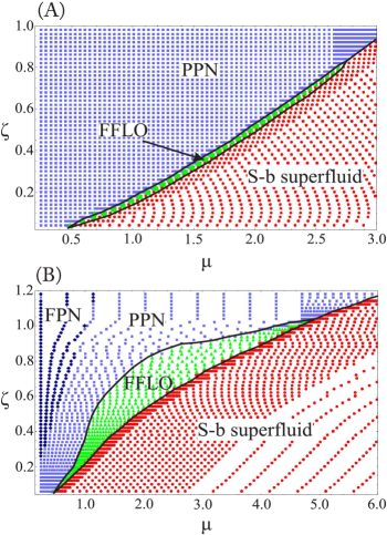
Figure 1: Comparison between the phase diagram in the $\left(\mu,\zeta\right)$-plane ($\mu$ and $\zeta$ are in units $E_{0}=\frac{\hbar^{2}}{2ma_{s}^{2}}$) of (A) an imbalanced Fermi gas in 3D, and (B) an imbalanced Fermi gas in 3D, subjected to a 1D optical potential. Both phase diagrams are constructed based on a finite set of points in the $\left(\mu,\zeta\right)$-plane. For each point, the ground state of the system is determined. There are four possible ground states: a spin-balanced (S-b) superfluid (red circles), the FFLO phase (green triangles), the partially polarized normal (PPN) phase (light blue squares) and the fully polarized normal (FPN) phase (dark blue diamonds). The presence of the 1D optical potential leads to a significant enlargement of the FFLO region. We used $s=\frac{V_{0}}{E_{R}}=5$ and $\lambda=1200$nm for the depth and wave length of the optical potential, and $\left|a_{s}\right|=500$nm for the s-wave scattering length.

In both these phase diagrams the ground state of the system is determined for a discrete set of $\left(\mu,\zeta\right)$-points and each of these points is displayed. We chose this type of visualization so that later on in this paper, the transformation to the phase diagram at fixed densities will be clarified by the transformation of the set of $\left(\mu,\zeta\right)$-points to a set of $\left(\frac{1}{k_{F}a_{s}},P\right)$-points, where $P$ denotes the polarization. In both phase diagrams in figure 1, the system is always in a spin-balanced superfluid state when $\zeta=0$. This is not visible in Fig. 1 since in this figure $\zeta\geq 0.06$. For small values of the total chemical potential $\mu$ ($\mu\leq 0.5$ in Figs. 1 (A) and (B)), the system makes a transition into a partially polarized normal state when $\zeta$ becomes of the order of the gap $\Delta$. For larger values of $\mu$, the system goes through all three different states when the imbalance chemical potential $\zeta$ is increased from zero. For low values of $\zeta$, the system remains a spin-balanced superfluid. This means that a finite energy is needed in order to convert particles from one spin species to the other. The minimal amount of energy that is required for this conversion increases when the total chemical potential increases. For high enough values of $\zeta$ the Fermi gas becomes polarized. At this point the system makes a transition into the FFLO state, both in figure 1 (A) and (B). Characteristic of the FFLO state is that it has an oscillating order parameter Fulde Ferell ; Larkin Ovchinnikov . This order parameter is enhanced by the presence of the 1D potential, which results in a much larger FFLO region in Fig. 1 (B) when compared to the case without the optical potential in Fig. 1 (A). When the imbalance chemical potential $\zeta$ increases further, the system will go over into a partially polarized (PPN) state and eventually into a fully polarized (FPN) state, and superfluidity is destroyed.

In the phase diagram in Fig. 1, we made the following choice for the depth $s=V_{0}/E_{R}$ and for the wave length $\lambda$ of the optical potential: $s=5$ and $\lambda=1000nm$, which are both realizable in current experiments. The depth of the optical potential must be chosen carefully, because the dispersion relation (3) that is used in our description is only valid in the tight-binding limit. This will be discussed in more detail in Sec. III.1. Both parameters $s$ and $\lambda$ correspond to specific values of $\delta$ and $Q_{L}$, which are defined in expression (3). Since we use units of scattering length, a fixed value of this quantity has to be chosen, in order to compute the values of $\delta$ and $Q_{L}$. Here we choose $\left|a_{s}\right|=500nm$, which corresponds to a situation close to a Feshbach resonance.

II.2 Phase diagram at fixed densities

In the previous section, we chose to construct a phase diagram at fixed chemical potentials $\mu$ and $\zeta$. This is not the only possible choice. Another possibility is to work at fixed total density $n=n_{\uparrow}+n_{\downarrow}$ and fixed polarization $P=\left(n_{\uparrow}-n_{\downarrow}\right)/\left(n_{\uparrow}+n_{\downarrow}\right)$, which is equivalent to fixing the density of both spin species $n_{\uparrow}$ and $n_{\downarrow}$. To transform between these two descriptions, the following number equations have to be solved:

$$\left\{\begin{array}[c]{c}n=-\left.\dfrac{\partial\Omega_{sp}\left(\mu,\zeta;\Delta,Q\right)}{\partial\mu}\right|_{\zeta}\\ \delta n=-\left.\dfrac{\partial\Omega_{sp}\left(\mu,\zeta;\Delta,Q\right)}{\partial\zeta}\right|_{\mu}\end{array}\right..$$ (5)

In principle, we need to use the chain rule in (5), since $\Delta$ and $Q$ are separate variables that depend on $\mu$ and $\zeta$. But the saddle-point condition (4) will make these terms disappear. If fluctuations around the saddle point are taken into account, these extra terms will remain. The inclusion of fluctuations around the saddle point lies beyond the scope of this paper. Starting from the phase diagram at fixed chemical potentials in figure 1 (B), the phase diagram at fixed densities can now be constructed. Every point in the phase diagram depicted in figure 1 (B) corresponds to a set of values for the parameters $\left(\mu,\zeta;\Delta,Q\right)$. Inserting these values into both equations in (5) yields the density $n$ and the density difference $\delta n=n_{\uparrow}-n_{\downarrow}$. The latter can also be written as the polarization $P=\delta n/n$. The final step is to find the interaction strength $\left(k_{F}a_{s}\right)^{-1}$ that corresponds to the density $n$. Since the scattering length $a_{s}$ is kept constant, this can be done by using the following expression that relates the density to the Fermi wave vector $k_{F}$:

$$n=\left\{\begin{array}[c]{c}\dfrac{Q_{L}}{2\pi^{2}}\left(k_{F}^{2}-\delta\right)~{}\left(E_{F}\geq 2\delta\right)\\ \dfrac{Q_{L}}{2\pi^{3}}\left[\left(k_{F}^{2}-\delta\right)\arccos\left(\dfrac{\delta-k_{F}^{2}}{\delta}\right)+\delta\sqrt{1-\left(\dfrac{\delta-k_{F}^{2}}{\delta}\right)^{2}}\right]~{}\left(E_{F}<2\delta\right)\end{array}\right..$$ (6)

This expression (6) is derived by calculating the number of particles at temperature zero that have an energy that lies lower than the Fermi energy, where the particles are assumed to have a dispersion relation given by (3). The procedure outlined above yields the phase diagram at fixed density and at fixed polarization, which is shown in figure 2. Each point on this phase diagram corresponds to a point on the $\left(\mu,\zeta\right)$-phase diagram in figure 1 (B).

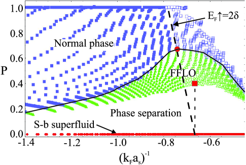
Figure 2: Phase diagram of an imbalanced Fermi gas in 3D, subjected to a 1D optical potential, at fixed density and fixed polarization P. The dimensionless parameter $\left(k_{F}a_{s}\right)^{-1}$ characterizes the interaction strength. Each point in this phase diagram is a transformation of a corresponding point in the phase diagram in figure 1 (B). At polarization zero, the system is in the spin-balanced (S-b) superfluid phase. When polarization becomes finite, there is a region where no points exist. This means that no combination of density and polarization can solve the number equations, and the system separates into two phases: a spin-balanced superfluid component and an FFLO component. Interestingly, both the boundary between the phase separation region and FFLO, and between FFLO and the normal phase have a maximum (indicated by a red square and a red circle respectively). The dashed oblique line indicates the boundary where the Fermi energy of the majority spins becomes equal to the top of the first Bloch band, which is equal to $2\delta$. The empty blue squares (normal phase) and empty green triangles (FFLO) indicate that the Fermi energy of the majority spins lies higher than the top of the first Bloch band. The vertical dashed line indicates the value of the interaction strength where the Fermi energy at polarization zero becomes equal to the top of the first Bloch band. Both dashed lines intersect with one of the two indicated maxima. ($s=5,$ $\lambda=1200$nm, and $\left|a_{s}\right|=500$nm)

In the case of zero polarization, the system is in the spin-balanced superfluid state. Figure 2 shows that there exists a portion of the phase diagram at finite polarization, where no points are present. Mathematically, this corresponds to the case when there exists no combination of density and polarization that can satisfy both number equations (5). Physically, this is a state where the system separates into two different phases: a spin-balanced superfluid phase and an FFLO phase, where the latter is being pushed out of the former. When polarization increases further, the system makes a transition into the FFLO state. Figure 2 also shows that when the interaction strength increases, both the boundary between the phase separation region and the FFLO state and the boundary between the FFLO state and the normal state, lie at higher values of polarization. Interestingly though, for both boundaries there exists a critical interaction strength at which this polarization becomes maximal. These two maxima are indicated by a red square and a red circle respectively in figure 2. If the interaction strength becomes larger than these two critical values, both the region of phase separation and the FFLO region seem to shrink. This counterintuitive effect will be discussed in the next section. When polarization increases further, the energy cost of forming pairs with finite momentum will eventually become too high and the system will make a transition into a normal Fermi gas. The points with polarization $P=1$ correspond to the fully polarized region in Fig. 1. We now have given a general overview of the phase diagrams of an imbalanced 3D Fermi gas subjected to a 1D potential. In the next section we will investigate the effects of the properties of the optical potential on the FFLO state.

III Effects of the 1D potential on the FFLO state

III.1 Role of the wave length and the depth of the optical potential

There are two parameters that determine the properties of the 1D optical potential: the potential depth $s$, and the wave length $\lambda$. Before discussing the effect of these parameters, it is important to know to which intervals they are limited in our current treatment. For the wave length, we take realistic values corresponding to present day experiments: $\lambda\in\left[600nm,1200nm\right]$. We have to be careful, however, when choosing values for the depth of the optical potential. There are two physical reasons to set a lower boundary to this depth. Firstly, since the optical potential is described by a tight-binding dispersion relation (Eq. 3), the depth of the potential must be large enough to justify this approximation. To quantify this, we calculated the energy spectrum of a particle in a periodic potential, and compared it to the tight-binding dispersion given by (3). For completeness, we added a concise overview of this calculation in appendix A. This calculation shows that the error made by using expression (3) for the dispersion is less than five percent when $s\geq 4$. Secondly, by using the dispersion relation (3), we only take into account the lowest Bloch band. This description is justified as long as the system has a Fermi energy which lies below the second Bloch band. A Fermi energy that lies between the top of the first Bloch band and the bottom of the second Bloch band is allowed, since the dispersion in the direction perpendicular to the direction of the optical potential is still the same as in the free 3D Fermi gas case. We have verified that by considering a potential depth $s\geq 4$, the system has a Fermi energy that lies below the bottom of the second Bloch band, for all cases considered in this paper. Based on this analysis, we will use the lower boundary $s=4$ for the potential depth throughout the rest of this paper. There is also a reason to set an upper limit to the depth of the optical potential. When the potential becomes too deep, the 3D Fermi gas will transition into a series of weakly-coupled two-dimensional (2D) pancakes. Such a 2D Fermi gas must be described using a different renormalized interaction strength Artikels 2D tunneling . We therefore choose $s$ to lie between 4 and 6, so that both the 3D description and the tight-binding approximation are justified.

We now proceed to investigate the effects of both optical potential parameters $\lambda$ and $s$. Figure 3 shows several phase diagrams at fixed density and polarization, for an imbalanced Fermi gas in 3D subjected to a 1D potential, for various values of both parameters $\lambda$ and $s$.

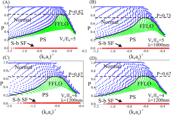
Figure 3: Overview of several phase diagrams of an imbalanced Fermi gas in 3D subjected to a 1D optical potential, for different values of the depth $s$ and the wave length $\lambda$ of the potential. The maximal polarization P at which the FFLO state can exist (indicated by a dashed horizontal line) increases when the wavelength of the optical potential becomes smaller. At constant wave length, the depth of the optical potential does not have an influence on this maximal polarization, at least within the range $4\leq s\leq 6$ that is considered here. (S-b SF = spin-balanced superfluid, PS = phase separation)

In Figs. 3 (A), (B), and (C) the wave length of the optical potential is varied. These three figures show that the maximal polarization at which the FFLO state can exist increases when the wave length of the optical potential becomes smaller. This effect agrees with our expectations and can best be explained in terms of the Fermi surfaces in momentum space. When an imbalance exists between spin-up and spin-down particles, an energy gap opens up between the Fermi surfaces of the two spin species. This is akin to a Zeeman-splitting effect. In order to bridge this gap and to let particles pair with the same energy, the FFLO state forms pairs with a finite momentum $Q$. The larger the imbalance, the larger the energy gap becomes and the larger $Q$ has to be. In Ref. Devreese Klimin en Tempere (2011) we demonstrated that the wave vector of the FFLO state cannot become larger than the wave vector of the optical potential. Since a smaller wave length corresponds to a larger wave vector, the maximal value of the wave vector $Q$ that can be attained by the FFLO state increases when the wave length of the optical potential decreases. This means that a larger energy gap can be bridged and thus a larger polarization can be accommodated. Figures 3 (C) and 3 (D) show the phase diagram of the system at the same wave length but at different potential depth. In both figures, the maximal polarization of the FFLO state is equal. We conclude that only the wave length of the optical potential has an influence on the capability of the system to remain in the FFLO state while being polarized, at least within the small range of potential depth $s$ that is considered here.

III.2 Effect of the edge of the Brillouin zone

One effect that is visible throughout all phase diagrams in figures 2 and 3, is that when the interaction strength exceeds a certain critical value, both the region of phase separation and the FFLO region become less stable with respect to polarization (i.e. the maximal polarization at which they can exist, decreases) . This can be seen by the fact that both the boundary between the phase separation region and the FFLO state and the boundary between the FFLO state and the normal state have a maximum (indicated by a red square and a red circle respectively in figure 2). Moreover, these two maxima seem to correspond to different values of the interaction strength. This effect is counterintuitive, because when the interaction strength increases, the binding energy of the fermion pairs increases likewise, which in general should strengthen superfluidity, not weaken it.

This effect is explained with the help of figure 2. In this figure, the empty blue squares (normal state) and the empty green triangles (FFLO state) indicate that the Fermi energy of the majority spins lies higher than the top of the first Bloch band, which is equal to $2\delta$. The boundary at which the Fermi energy of the majority spins becomes equal to the top of the first Bloch band is indicated by the dashed oblique line. The maximum polarization under which the FFLO state can exist (red circle), lies exactly at this line. Furthermore, the vertical dashed line indicates the value of the interaction strength at which the Fermi energy at polarization zero becomes equal to the top of the first Bloch band. This dashed vertical line intersects with the maximum polarization under which the phase separation region can exist (red square). The reason why each of these two dashed lines intersects with one of the two maxima can be explained as follows. Consider the case which is shown schematically in Fig. 4. Figure 4 (A) shows the Fermi surface of both spin-up and spin-down particles at polarization zero. In order for the system to become superfluid, pairing occurs between particles that lie in a band with thickness $\Delta$ around the Fermi energy. When these pairing bands of the spin-up and spin-down particles overlap, pairing is possible and the system is in the superfluid state. When polarization is introduced, a gap arises between the two Fermi surfaces, as indicated in figure 4 (B). As long as this gap is smaller than $\Delta$, there is overlap of the pairing bands, and superfluidity is possible in principle. When the polarization becomes too large, the overlap disappears and BCS superfluidity is no longer possible. In order to remain superfluid, the system can transition into the FFLO state, which translates the Fermi surface of the minority spins so that it locally lies on the Fermi surface of the majority spins, making pairing possible again (see Fig. 4 (B)). This allows the system to remain superfluid, at the cost of paying some energy to form particles with finite center-of-mass momentum. This is the case for a 3D Fermi gas, but when a 1D potential is added, an additional effect comes into play. When the density and/or polarization is high enough so that the Fermi surface of the majority spins lies at the edge of the first Brillouin zone (this is true for the area at the right side of the dashed oblique line in Fig. 2), pairing at this Fermi surface becomes more difficult, because for $k_{z}>Q_{L}$, there are no available states (see Fig. 4 (C)). Hence, the formation of an FFLO-type superfluid phase will be hindered. This now explains why, at equal polarization, the normal phase becomes favored over the FFLO phase when the interaction strength exceeds the value corresponding to the situation where the Fermi energy of the majority spins equals the top of the first Bloch band (indicated by a red circle in Fig. 2). The question can be raised whether the FFLO state can still exist if the fermion pairs acquire a momentum in the $x$ or $y$ direction, since there exists no Brillouin zone in these directions. We did not treat this case in our paper because we assumed the FFLO momentum to be of the form $Q=\left(0,0,Q_{z}\right)$.

In the case of figure 4 (C), BCS superfluidity can still exist, because when the Fermi surface of the minority spins is not translated, pairing does not occur at the boundary of the first Brillouin zone. However, when the density becomes high enough, even the Fermi surface of the particles at zero polarization will lie at this edge. This situation is depicted in figure 4 (D). For this and for higher densities, pairing of BCS superfluidity will also occur at the edge of the Brillouin zone and it will suffer the same problem as the FFLO state. This effect can be seen in Fig. 2 from the fact that, at equal polarization, the FFLO state becomes favored over the spin-balanced superfluid phase, when the value of the interaction strength increases above the value corresponding to the situation where the Fermi energy at zero polarization equals the top of the first Bloch band (indicated by a red square in Fig. 2).

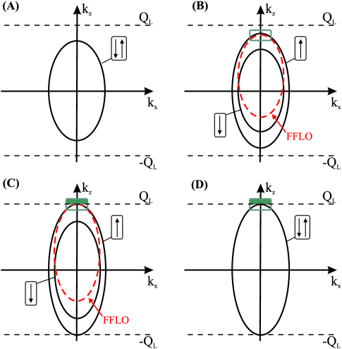
Figure 4: Schematic representation of the pairing mechanisms in an imbalanced 3D Fermi gas subjected to a 1D optical potential. For the sake of clarity, we have omitted the y direction. (A) The Fermi surfaces of the spin-up and the spin-down particles at polarization zero. Pairing occurs in a band with thickness $\Delta$ around the Fermi energy and BCS superfluidity is possible. (B) When polarization is introduced, a gap is created between the Fermi surfaces of both spin species. If this gap becomes too big, there will be no overlap between the pairings bands around the Fermi surfaces. The system can solve this by translating the minority Fermi surface (dashed red ellipsoid) so that locally, both Fermi surfaces are re-aligned (indicated by a green rectangle). (C) When the density increases, the Fermi surface of the majority spins (here spin-up) will lie at the edge of the first Brillouin zone. This will hinder FFLO-like pairing because no states are available at $k_{z}>Q_{L}$. (D) Above a critical density, the Fermi surface lies at the edge of the Brillouin zone even for polarization zero. At this point, BCS superfluidity will also be hindered.

IV Conclusions

We have investigated the effects of a 1D optical potential on the FFLO state in an imbalanced Fermi gas in 3D. To allow for a direct connection with the experiments, we constructed the phase diagram of the system, both at fixed chemical potentials and at fixed densities of both spin species. Subsequently, we investigated the effects of the depth and the wave length of the optical potential on the FFLO state. It was shown that this state can exist under a larger polarization, when the wave length of the optical potential becomes smaller. The depth of the optical potential did not have any appreciable effect, within the range that can be considered in our tight-binding approximation. By studying the phase diagram at fixed density we have discovered an unexpected effect. When the interaction strength exceeds a certain critical value, the maximal polarization at which both the FFLO phase and the phase separation region can exist decreases. The underlying reason was discussed in detail. We have found that when the density of the system becomes so high that the Fermi energy exceeds the top of the lowest Bloch band, superfluid pairing becomes hindered. This is because in that case, particles with the highest energy lie at the edge of the first Brillouin zone. Since no states exist outside of this zone, pairing is not possible and the superfluid state is suppressed. We expect this effect, along with the enhancement of the FFLO state, to be observable in experiments where a 1D optical potential is applied to an imbalanced Fermi gas in 3D.

Appendix A Range of optical potential depths that allow the tight-binding approximation

The energy spectrum of a particle in a periodic potential can be calculated using Schrödinger’s equation. The potential under consideration is given by

$$V\left(z\right)=sE_{R}\sin^{2}\left(Q_{L}z\right),$$ (7)

where $s$ is the depth of the optical potential in units of the recoil energy $E_{R}$ and $Q_{L}$ is the wave vector of the optical potential given by $Q_{L}=\pi/\lambda$. Given this potential, Schrödinger’s equation states that

$$\left[-\frac{\hbar^{2}}{2m}\frac{d^{2}}{dz^{2}}+sE_{R}\left(\frac{1-\cos\left(2Q_{L}z\right)}{2}\right)\right]\psi_{k}\left(z\right)=\varepsilon_{k}\psi_{k}\left(z\right).$$ (8)

Since we consider a particle in a periodic potential, Bloch’s theorem applies and we can re-write the wave function $\psi_{k}\left(z\right)$ as

$$\psi_{k}\left(z\right)=e^{ikz}u_{k}\left(z\right),$$ (9)

where $u_{k}\left(z\right)$ has the same periodicity as the potential. Because $u_{k}\left(z\right)$ is periodic, it can be written in a Fourier series

$$\psi_{k}\left(z\right) =e^{ikz}\left(\sum_{n}c_{n}e^{i\frac{2\pi n}{\lambda}z}\right)$$

$$=\sum_{n}c_{n}e^{i\left(k+2nQ_{L}\right)z}.$$ (10)

Substituting (10) in Eq. (8) yields

$$\sum_{n}\left[\frac{\hbar^{2}}{2m}\left(k+2nQ_{L}\right)^{2}+\frac{sE_{R}}{2}\right]c_{n}e^{i\left(k+2nQ_{L}\right)z}-\frac{sE_{R}}{2}\sum_{n}\left(\frac{e^{2iQ_{L}z}+e^{-2iQ_{L}z}}{2}\right)c_{n}e^{i\left(k+2nQ_{L}\right)z}$$

$$=\varepsilon_{k}\sum_{n}c_{n}e^{i\left(k+2nQ_{L}\right)z}.$$ (11)

Re-indexing the second sum over $n$ and identifying the coefficients on both sides in equation (11) leads to

$$\left[\frac{\hbar^{2}}{2m}\left(k+2nQ_{L}\right)^{2}+\frac{sE_{R}}{2}-\varepsilon_{k}\right]c_{n}-\frac{sE_{R}}{4}\left(c_{n+1}+c_{n-1}\right)=0.$$ (12)

This expression represents an infinite set of linear equations. In practice, it is enough to consider five equations, since the contributions of the eigenvectors $c_{n}$ decreases exponentially for large $n$. Solving equation (12) numerically yields the exact energy spectrum of a particle in a periodic potential, given by (7). Figure 5 shows a comparison between this exact spectrum and the corresponding dispersion relation in the tight-binding limit, given by (3). For $s\leq 2$ the difference is substantial, but for $s\geq 4$, the approximation deviates less than 5 percent from the exact result. This justifies the approximation that we make by considering $s\geq 4$.

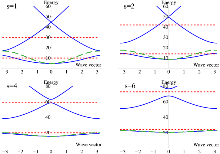
Figure 5: Comparison between the exact energy spectrum of a particle in a periodic potential (solid blue lines) and the dispersion relation calculated in the tight-binding limit (long-dashed green lines), given by expression (3). The horizontal short-dashed red lines indicate the two lowest energy levels of the harmonic oscillator, derived by approximating (3) to second order in the momentum. For $s\geq 4$, the difference between the exact energy spectrum and the tight-binding dispersion is less than 5%.

References

- (1) I. Bloch, J. Dalibard, and W. Zwerger, Rev. Mod. Phys. 80, 885 (2008).
- (2) M. Greiner, C. A. Regal, and D. S. Jin, Nature (London) 426, 537 (2003).
- (3) C. Chin, M. Bartenstein, A. Altmeyer, S. Riedl, S. Jochim, J. Hecker Denschlag, R. Grimm, Science 305, 1128 (2004).
- (4) M. W. Zwierlein, C. A. Stan, C. H. Schunck, S. M. F. Raupach, A. J. Kerman, and W. Ketterle, Phys. Rev. Lett. 92, 120403 (2004).
- (5) T.-L. Dao, A. Georges, J. Dalibard, C. Salomon, and I. Carusotto, Phys. Rev. Lett. 98, 240402 (2007).
- (6) I. Bloch, Nat. Phys. 1, 23 (2005).
- (7) M. Greiner and S. Fölling, Nature (London) 453, 736 (2008).
- (8) C. Chin, R. Grimm, P. Julienne, and E. Tiesinga, Rev. Mod. Phys. 82, 1225 (2010).
- (9) C. A. Regal, M. Greiner, and D. S. Jin, Phys. Rev. Lett. 92, 040403 (2004).
- (10) T. Bourdel, L. Khaykovich, J. Cubizolles, J. Zhang, F. Chevy, M. Teichmann, L. Tarruell, S. J. J. M. F. Kokkelmans, and C. Salomon, Phys. Rev. Lett. 93, 050401 (2004).
- (11) G. B. Partridge, K. E. Strecker, R. I. Kamar, M. W. Jack, and R. G. Hulet, Phys. Rev. Lett. 95, 020404 (2005).
- (12) C. A. R. Sá de Melo, M. Randeria and, J. R. Engelbrecht, Phys. Rev. Lett. 71, 3202 (1993).
- (13) M. W. Zwierlein, A. Schirotzek, C. H. Schunck, and W. Ketterle, Science 311, 492 (2006); M. W. Zwierlein, C. H. Schunck, A. Schirotzek, and W. Ketterle, Nature (London) 442, 54 (2006).
- (14) G. B. Partridge, W. Li, R. I. Kamar, Y. A. Liao, and R. G. Hulet, Science 311, 503 (2006).
- (15) Y. Shin, M. W. Zwierlein, C. H. Schunck, A. Schirotzek, and W. Ketterle, Phys. Rev. Lett. 97, 030401 (2006).
- (16) G. B. Partridge, W. Li, Y. A. Liao, R. G. Hulet, M. Haque, and H. T. C. Stoof, Phys. Rev. Lett. 97, 190407 (2006).
- (17) C. H. Schunck, Y. Shin, A. Schirotzek, M. W. Zwierlein, and W. Ketterle, Science 316, 867 (2007).
- (18) A. M. Clogston, Phys. Rev. Lett. 9, 266 (1962); B. S. Chandrasekhar, Appl. Phys. Lett. 1, 7 (1962).
- (19) W. Ketterle, Y. Shin, A. Schirotzek, and C. H. Shunk, J. Phys. Condens. Matter 21, 164206 (2009).
- (20) G. Sarma, J. Phys. Chem. Solids 24, 1029 (1963) ; W. V. Liu and F. Wilczek, Phys. Rev. Lett. 90, 047002 (2003).
- (21) K. B. Gubbels, M. W. J. Romans, and H. T. C. Stoof, Phys. Rev. Lett. 97, 210402 (2006); L. He and P. Zhuang, Phys. Rev. B. 79, 024511 (2009).
- (22) P. F. Bedaque, H. Caldas, and G. Rupak, Phys. Rev. Lett. 91, 247002 (2003); J. Tempere, S. N. Klimin, and J. T. Devreese, Phys. Rev. A 78, 023626 (2008).
- (23) P. Fulde and R. A. Ferrell, Phys. Rev. 135, A550 (1964).
- (24) A. I. Larkin and Y. N. Ovchinnikov, Zh. Eksp. Teor. Fiz. 47, 1136 (1964) [Sov. Phys. JETP 20, 762 (1965)].
- (25) Y. Liao, A. S. C. Rittner, T. Paprotta, W. Li, G. B. Partridge, R. G. Hulet, S. K. Baur, and E. J. Mueller, Nature 467, 567 (2010).
- (26) H. Hu and X. J. Liu, Phys. Rev. A 73, 051603(R) (2006).
- (27) D. E. Sheehy and L. Radzihovsky, Ann. of Phys. 322, 1790 (2007); L. Radzihovsky and D. E. Sheehy, Rep. Prog. Phys. 73, 076501 (2010).
- (28) T. K. Koponen, T. Paananen, J.-P. Martikainen, and P. Törmä, Phys. Rev. Lett. 99, 120403 (2007).
- (29) Y. L. Loh and N. Trivedi, Phys. Rev. Lett. 104, 165302 (2010).
- (30) J. P. A. Devreese, S. N. Klimin, and J. Tempere, Phys. Rev. A 83, 013606 (2011).
- (31) H. Kleinert, Path Integrals in Quantum Mechanics, Statistics, Polymer Physics, and Financial Markets, 5th ed.(World Scientific, Singapore, 2002).
- (32) L. Pezzè, L. Pitaevskii, A. Smerzi, S. Stringari, G. Modugno, E. de Mirandes, F. Ferlaino, H. Ott, G. Roati, and M. Inguscio, Phys. Rev. Lett. 93, 120401 (2004).
- (33) M. Iskin and C. A. R. Sá de Melo, Phys. Rev. B 97, 100404 (2006).
- (34) D. E. Sheehy and L. Radzihovsky, Phys. Rev. Lett. 96, 060401 (2006).
- (35) M. Wouters, J. Tempere, and J. T. Devreese, Phys. Rev. A 70, 013616 (2004); J. Tempere, J. Low. Temp. Phys. 150, 636 (2008).