Spectral optical monitoring of 3C 390.3 in 1995-2007: II. Variability of the spectral line parameters

Abstract

Context. A study of the variability of the broad emission-line parameters of 3C390.3, an active galaxy with the double-peaked emission-line profiles, is presented. Here we give a detail analysis of variation in the broad H$\alpha$ and H$\beta$ emission-line profiles, the ratios, and the Balmer decrement of different line segments.

Aims. With investigation of the variability of the broad line profiles we explore the disk structure, that is assumed to emit the broad double-peaked H$\beta$ and H$\alpha$ emission lines in the spectrum of 3C390.3.

Methods. We divided the observed spectra in two periods (before and after the outburst in 2002) and analyzed separately the variation in these two periods. First we analyzed the spectral emission-line profiles of the H$\alpha$ and H$\beta$ lines, measuring the peak positions. Then, we divided lines into several segments, and we measured the line-segment fluxes. The Balmer decrement variation for total H$\alpha$ and H$\beta$ fluxes, as well as for the line segments has been investigated and discussed. Additionally, we modeled the line parameters variation using an accretion disk model and compare our modeled line parameter variations with observed ones.

Results. We compared the variability in the observed line parameters with the disk model predictions and we found that the variation in line profiles and in the line segments corresponds to the emission of a disk-like BLR. But, also there is probably one additional emission component that contributes to the H$\alpha$ and H$\beta$ line center. We found that the variation in the line profiles is caused by the variation in the parameters of the disk-like BLR, first of all in the inner (outer) radius which can well explain the line parameter variations in the Period I. The Balmer decrement across the line profile has a bell-like shape, and it is affected not only by physical processes in the disk, but also by different emitting disk dimension of the H$\alpha$ and H$\beta$ line.

Conclusions. The geometry of the BLR of 3C390.3 seems to be very complex, and inflows/outflows might be present, but it is evident that the broad line region with disk-like geometry has dominant emission.

1 Introduction

The broad emission lines (BELs) are often observed in optical and ultraviolet spectra of acitve galactic nuclei (AGN). The study of the profiles and intensities of BELs can give us relevant information about the geometry and physics of the broad line region (BLR). The physics and geometry of the BLR are uncertain and investigation of BEL shape variability in a long period is very useful for determination of the BLR nature. The profiles of the BELs in AGN can indicate the geometry of emitting plasma in the BLR (see e.g. , 2000, 2004, 2009, 2010, etc.).

Particularly, very interesting objects are AGNs with unusual broad emission-line profiles, where broad Balmer lines show double peaks or double ”shoulders”, so called double-peaked emitters. The double peaked line profiles may be caused by an accretion disk emission. On the other hand, the presence of an accretion-disk emission in the BLR is expected, and double-peaked line profiles of some AGN indicate this (, 1988, 1994, 2004, 2009). One of the well known AGN with broad double-peaked emission lines in its spectrum is the radio-loud active galaxy 3C 390.3. Although, the double-peaked line profiles can be explained by different hypothesis (see e.g. , 1991), as e.g. super-massive binary black holes (, 1996), outflowing bi-conical gas streams (, 1996)), it seems that in this case a disk emission is present in the BLR (, 2010, hereinafter Paper I). There is a possibility that a jet emission can affect the optical emission in 3C 390.3 (, 2010), and some perturbations in disk could be present (, 2010) and they can also affect the double-peaked line profiles.

Long-term variability in the line/continuum flux as well as in the line profiles is observed in objects with broad double peaked lines (see e.g. , 1988, 2001, 2002, 2010, 2010, 2010). Long-term variability of broad line profiles is intriguing because it is usually unrelated to more rapid changes in the continuum flux, but probably is related to physical changes in the accretion disk, as e.g. brightness of some part of the disk, or changes in the disk size and distance to the central black hole. The double-peaked broad line profile variability can be exploited to test various models for the accretion disk (as e.g. circular or elliptical). Moreover, the double-peaked broad line studies can provide important information about the accretion disk, as e.g. inclination, dimension and emissivity of the disk as well as probes of dynamical phenomena that may occur in the disk (see in more details , 2009, and reference therein).

In Paper I we have presented the results of the long-term (1995–2007) spectral monitoring of 3C~390.3. We have analyzed the light curves of the broad H$\alpha$ and H$\beta$ line fluxes and the continuum flux in the 13-year period. We also found that quasi-periodical oscillations (QPO) may be present in the continuum and H$\beta$ light curves. We studied averaged profile of the H$\alpha$ and H$\beta$ line in two periods (Period I from 1995 to 2002, and Period II from 2003 to 2007) and their characteristics (as e.g. peaks separation and their intensity ratio, or FWHM). From the cross-correlations (ICCF and ZCCF) between the continuum flux and H$\beta$ and H$\alpha$ lines we found the lag of $\sim$95 days for H$\beta$ and $\sim$120 days for H$\alpha$ (see Paper I for details). We concluded that the broad emission region has disk-like structure, but there could probably exists an additional component, non-disk or also disk-like, with different parameters that contributes to the line emission. We found a differences in the H$\alpha$ and H$\beta$ line profiles before and after the beginning of the activity phase in 2002, consequently we divided our spectra into two periods (before March 05, 2002 – Period I and after that – Period II, see Paper I).

In this paper we study in more details the H$\alpha$ and H$\beta$ line profiles and ratios, taking into account the changes during the monitoring period. The aim of this paper is to investigate the changes in the the BLR structure of 3C 390.3 that cause the line profile variations. To perform this investigation we analyzed the peak separation variations, variations in line segments and variation in Balmer decrement. Using a relatively simple disk model, we try to explain qualitatively the changes in disk structure that can cause the line parameter variations.

The paper is organized as follow: in §2 we describe of our observations; in §3 we present the analysis of the H$\alpha$ and H$\beta$ line profiles variability, the peak-velocity variability and Balmer decrement; in §4 we study the line-segment variations; in §5 the Balmer decrement variation is analyzed; in §6 we discuss obtained results , and finally in §7 we outline our conclusions.

2 Observations

In 1995-2007 spectra of 3C 390.3 were taken with the 6 m and 1 m telescopes of the SAO RAS and with INAOE’s 2.1 m telescope of the ”Guillermo Haro Observatory” (GHO) at Cananea, Sonora, México and with a long slit spectrographs, equipped with CCD detector arrays. The typical wavelength interval covered was from 4000 Å  to 7500 Å, the spectral resolution varied between (4.5-15)  Å. Spectra were scaled using the [O iii] $\lambda\lambda$4959+5007 (for blue spectra) and the [OI]6300A (for red spectra) integrated line flux under the assumption that fluxes of this lines did not change during the time interval covered by our observations (1995–2007). The narrow components of H$\alpha$ and H$\beta$ were removed by applying the modified method of (1992) (see also , 2004) using the spectral template for narrow components as reference spectrum. More details about observations can be found in Paper I.

3 Analysis of the broad line profiles

In Paper I we explained the continuum and narrow line subtraction in order to obtain only the broad H$\alpha$ and H$\beta$ line profiles, and here that procedure will not be repeated. Using only broad line component we analyze the line parameters: month- and year- averaged line profiles (see Figs. 1–3, Figs. 2–3- available electronically only), the position (and separation) of prominent peaks, the fluxes of the line segments and the H$\alpha$/H$\beta$ ratios (or Balmer decrement – BD). In this section we first give the analysis of the observed broad line parameters, and after that we analyze the corresponding modeled line parameter, obtained using an accretion disk model, in order to learn about changes in the disk structure which may cause the line parameter variability.

Figure 1: The month-averaged profiles of the H$\alpha$ and H$\beta$ broad emission lines in the period 1995–2007. The abscissa (OX) shows radial velocities relative to the narrow component of H$\alpha$ or H$\beta$ line. The ordinate (OY) shows the line flux in units of $10^{-16}{\rm erg\ cm^{-2}s^{-1}}$Å^-1.

2

Figure 2: The year-averaged profiles (solid line) and their rms (dashed line) of the H$\alpha$ broad emission line in 1995–2007. The abscissa (OX) shows the radial velocities relative to the narrow component of the H$\alpha$ line. The ordinate (OY) shows the flux in units of $10^{-16}{\rm erg\ cm^{-2}s^{-1}}$Å^-1.

3

Figure 3: The same as in Fig. 2, but for H$\beta$ broad emission line.

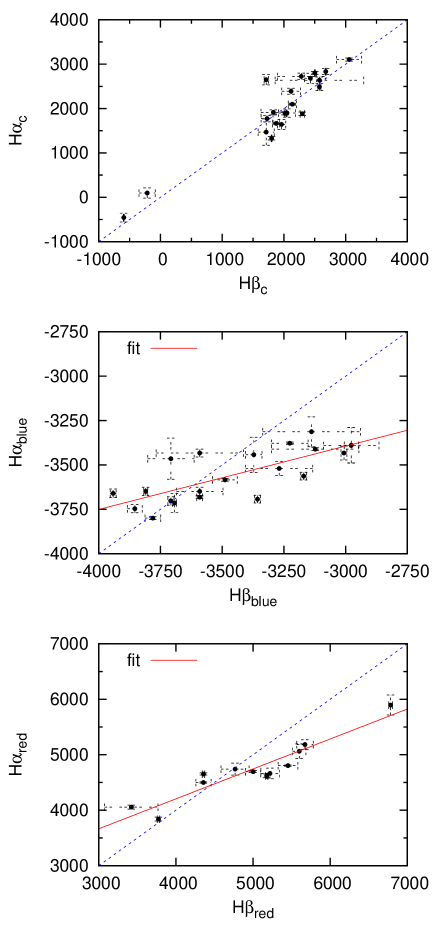
Figure 4: The H$\alpha$ vs. H$\beta$ peak velocity for the central (top), blue (middle) and red (down) peak. The dashed line represents expected function for equal peak position in both lines, while solid line represents the best fit of the measured data.

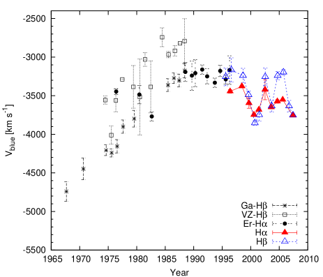
Figure 5: The annual averaged radial velocities of the blue peak. The different symbols represent: stars - the H$\beta$ data from (1996), open squares - the H$\beta$ measurements given in (1991), year-averaged to match other data, full circles - the H$\alpha$ data from (1997), open and full triangles - our data for H$\beta$ and H$\alpha$, respectively.

As reported in Paper I there is a differences in the H$\alpha$ and H$\beta$ line profiles before and after the beginning of the activity phase in 2002. Therefore, we consider separately line profiles obtained in the period before March 05, 2002 (Period I, JD 2 452 339.01 according the minimum in H$\beta$) and after that date (Period II, see Paper I). Also, we found that observations in 2001 and 2002 have sometimes closer characteristics as the data in Period II, therefore in some plots we marked separately these observations as 2001–2002.

3.1 The averaged profiles of the H$\alpha$ and H$\beta$ broad emission lines

It was also reported in Paper I that the line profiles of H$\alpha$ and H$\beta$ were changing during the monitoring period. In Fig. 1, we show the month- and in Figs. 2 and 3 (available electronically only) year-averaged profiles of the H$\alpha$ and H$\beta$. As it can be seen in Fig. 1 the line profiles of H$\alpha$ (left) and H$\beta$ (right) vary, showing clearly two, and sometimes three peaks. Similar variations can be seen from the year-averaged profiles (see Fig. 2 for H$\alpha$ and Fig. 3 for H$\beta$). Note here that in both periods the blue peak is higher as it is expected in the case of a relativistic accretion disk. The most interesting is the central peak at the zero velocity (clearly seen in 1995 and 1996) that may indicate perturbation in the disk or an additional emitting region. We found that this central peak (sometimes weaker) exists almost always during both periods, therefore we measured the position of the blue, central and red peak. Our measurements are given in Table 1. Sometimes the red peak could not be properly measured (since it was too weak or even absent), thus in that case the measurements are not given in Table 1. The measurements show that the position of the peaks are changing, and as can be seen in Fig. 4 changes are higher in the H$\beta$ than in H$\alpha$ line. It is interesting that the position of the blue peak varies around several hundreds km s^-1 (e.g. in H$\alpha$ it is -3550$\pm$250 km s^-1, in H$\beta$ -3500$\pm$400 km s^-1), while the position of the red peak has higher variation (for H$\alpha\ \sim$ +5000$\pm$ 1000 km s^-1, and for H$\beta\ \sim$ 5250$\pm$1700 km s^-1). This may indicate that the emission is coming relatively close to the central black hole.

There is a difference between the H$\alpha$ and H$\beta$ red and blue peak velocities (see Fig. 4), that can be expected due to the stratification of the disk, i.e. the different dimensions of the disk region that emits H$\alpha$ or H$\beta$. It is interesting that the central peak seems to stay at similar position in both lines, i.e. as it can be seen in Fig. 4 (panel top) the points follow well the linear bijection function (represented as dashed line). This could indicate that the central peak is connected with some kind of perturbation in a disk or an additional region that in the same way affects the H$\beta$ and H$\alpha$ line profiles. Note here that the so-called central peak was slightly shifted to the blue side (or close to the zero shift) in 1996–1997 (see Fig. 1), but after that this peak has been redshifted (between 1500 and 2500 km s^-1).

In order to compare the variability of the blue peak position during a longer period, in Fig. 5 we presented our measurements for the blue peak position and measurements obtained by (1991), (1996) and (1997). Note here that the estimates of the blue peak position in the H$\alpha$ line is more uncertain than in H$\beta$, due to the substraction of the atmosphere B-band (Paper I), while H$\beta$ is more uncertain in the red part due to subtraction of the [OIII] lines (see §4.1). As it can be seen in Fig. 5 the measurement follow well the previous observations, and there is an increase of the blue peak position velocity from 1970 to 1990 (1995), while after 1995, the the blue peak position velocity is slightly decreasing.

Table 1: Measurements of the peak position velocities (blue, central, red) from month-averaged H$\alpha$ and H$\beta$ profiles.

	H$\alpha$					H$\beta$
Year	Month	blue	central	red	$V_{\rm red}-V_{\rm blue}$	Month	blue	central	red	$V_{\rm red}-V_{\rm blue}$
		km/s	km/s	km/s	km/s		km/s	km/s	km/s	km/s
1996	Mar	-3520 $\pm$ 39	96 $\pm$ 115	3840 $\pm$ 35	7360 $\pm$ 74	Feb-Mar	-3269 $\pm$ 136	-216 $\pm$ 131	3773$\pm$ 16	7042 $\pm$ 152
1996	Jul	-3411 $\pm$ 8	-457 $\pm$ 100	4056 $\pm$ 35	7467 $\pm$ 43	Jun-Aug	-3123 $\pm$ 177	-595 $\pm$ 7	3422$\pm$ 346	6546 $\pm$ 523
1998	Feb	-3390 $\pm$ 100	2639 $\pm$ 71	-	-	May-Jun	-2977 $\pm$ 112	2575 $\pm$ 718	-	-
1998	Jul-Sep	-3378 $\pm$ 7	3104 $\pm$ 35	-	-	Jul	-3226 $\pm$ 74	3057 $\pm$ 202	-	-
1998	Dec	-3433 $\pm$ 22	2726 $\pm$ 71	-	-	Oct-Dec	-3591 $\pm$ 177	2283 $\pm$ 387	6359 $\pm$ 162	9950 $\pm$ 340
1999	Sep	-3465 $\pm$ 116	1914 $\pm$ 56	5896 $\pm$ 180	9361 $\pm$ 296	Aug-Oct	-3708 $\pm$ 94	1830 $\pm$ 201	6783 $\pm$ 24	10491 $\pm$ 118
2000	Jul	-3747 $\pm$ 23	2649 $\pm$ 117	5063 $\pm$ 133	8810 $\pm$ 156	Jul-Nov	-3854 $\pm$ 30	1713 $\pm$ 35	5599 $\pm$ 87	9453 $\pm$ 116
2001	Jan	-3660 $\pm$ 24	1665 $\pm$ 21	4803 $\pm$ 11	8463 $\pm$ 35	Jan-Mar	-3942 $\pm$ 12	1874 $\pm$ 56	5453 $\pm$ 128	9395 $\pm$ 140
2001	May-Jun	-3714 $\pm$ 53	2682 $\pm$ 112	5182 $\pm$ 88	8896 $\pm$ 141	May-Jun	-3693 $\pm$ 8	2429 $\pm$ 98	5673 $\pm$ 107	9366 $\pm$ 115
2001	Oct	-3693 $\pm$ 22	2390 $\pm$ 66	4803 $\pm$ 72	8496 $\pm$ 94	Oct-Nov	-3357 $\pm$ 12	2116 $\pm$ 151	-	-
2002	Feb-Mar	-3389 $\pm$ 100	1881 $\pm$ 41	4750 $\pm$ 26	8139 $\pm$ 126	Feb-Apr	-2977 $\pm$ 29	2298 $\pm$ 36	-	-
2002	Jun-Jul	-3313 $\pm$ 84	2098 $\pm$ 21	4662 $\pm$ 96	7975 $\pm$ 181	Jun	-3138 $\pm$ 198	2137 $\pm$ 67	-	-
2002	Oct-Nov	-3443 $\pm$ 99	1892 $\pm$ 36	4619 $\pm$ 35	8062 $\pm$ 134	Oct-Dec	-3372 $\pm$ 33	2020 $\pm$ 15	5176 $\pm$ 17	8548 $\pm$ 50
2003	May	-3649 $\pm$ 23	1899 $\pm$ 95	4695 $\pm$ 19	8344 $\pm$ 42	May-Jun	-3810 $\pm$ 8	2049 $\pm$ 139	5001 $\pm$ 100	8811 $\pm$ 108
2003	Sep-Oct	-3649 $\pm$ 23	1773 $\pm$ 71	4652 $\pm$ 19	8301 $\pm$ 42	Sep-Oct	-3591 $\pm$ 94	1727 $\pm$ 97	4358 $\pm$ 16	7948 $\pm$ 111
2004	Mar-Aug	-3584 $\pm$ 8	2487 $\pm$ 82	4500 $\pm$ 11	8085 $\pm$ 19	Mar-Jun	-3489 $\pm$ 50	2575 $\pm$ 25	4357 $\pm$ 99	7846 $\pm$ 149
2004	Dec	-3433 $\pm$ 39	2833 $\pm$ 70	4740 $\pm$ 109	8173 $\pm$ 147	Dec	-3007 $\pm$ 12	2678 $\pm$ 5	4767 $\pm$ 182	7773 $\pm$ 194
2005	Apr	-3563 $\pm$ 22	2801 $\pm$ 35	4533 $\pm$ 35	8095 $\pm$ 57	Apr-Jun	-3170 $\pm$ 12	2502 $\pm$ 6	-	-
2007	Jan	-3682 $\pm$ 7	1643 $\pm$ 113	-	-	Jan-Feb	-3591 $\pm$ 12	1961 $\pm$ 68	-	-
2007	Feb	-3703 $\pm$ 24	1329 $\pm$ 37	-	-	May-Jun	-3708 $\pm$ 12	1800 $\pm$ 6	-	-
2007	Aug-Nov	-3800 $\pm$ 8	1470 $\pm$ 297	-	-	Aug-Nov	-3781 $\pm$ 32	1713 $\pm$ 130	-	-

Figure 6: The modeled line profiles for the H$\alpha$ (top) and H$\beta$ (bottom) lines for different disk parameters (noted in the plots).

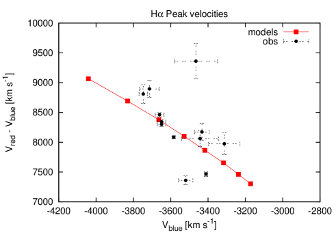
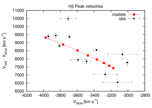
Figure 7: The difference between the blue and read peak velocities vs. the blue peak velocity for H$\alpha$ (top) and H$\beta$ line (bottom). The model parameters are marked with full squares, while observations are denoted with full circles.

3.2 Simulation of the line parameters variations

One can fit the broad double peaked line profiles to extract some disk parameters (see e.g. , 1994, 2004, 2008, 2010, 2010, etc.), but here, since we have a large set of observational data, we will use a simple model to simulate variations in different disk parameters and give some qualitative conclusions.

To qualitatively explain the changes in the disk structure that can cause the line parameter variations, we simulate the disk emission, using a disc model given by (1989) and (1989). The model assumes a relativistic, geometrically thin and circular disk (see in more details , 1989, 1989). Note here that in this model relativistic effects are approximatively included and the limit of the inner radius is $R_{inn}>100$ R_g ($R_{g}=GM/c^{2}$ – gravitational radius), but the estimated inner radius in the case of 3C390.3 is significantly larger (see , 2008), consequently, the model given by (1989) and (1989) can be properly used, i.e. it is not necessary to include a full relativistic calculation (as e. g. in , 2010).

To obtain the double-peaked line profiles we generated the set of different disk-like line profiles. For the starting parameters of the H$\alpha$ line we used the results of (2008). They obtained the following disk parameters from fitting the observed H$\alpha$ line of 3C 390.3: the inner radius $R_{\rm inn}=450\ R_{\rm g}$, the outer radius $R_{\rm out}=1400\ R_{\rm g}$, the disk inclination $i=27\deg$, the random velocity in the disk $\sigma=1300\ {\rm km\ s^{-1}}$, with the emissivity $r^{-q}$, where $q=3$ is assumed. To model the parameters for the H$\beta$ line, we took into account the results from Paper I that the dimension of the H$\alpha$ emitting region is $\sim$ 120 light days, and of H$\beta$ is $\sim$ 95 light days, consequently we proportionally (95/120) rescaled the H$\beta$ disk parameters for outer radius (i.e. $R_{\rm out}=1200\ R_{\rm g}$) keeping other parameters as in the case of the H$\alpha$ disk. Note here that we assumed that the inner radius for both, H$\alpha$ and H$\beta$ is the same. It is an approximation, but one may expect that the plasma conditions (temperature and density) are probably changing fast in the inner part of disk, therefore at some distance from the black hole, the plasma has such conditions that can emit Balmer lines (i.e. recombination stays effective). On the other side, at larger distances from the black hole, the conditions in plasma are slowly changing (as a function of radius) and from some distance, due to the probability of transitions, there may be significant emission in the H$\alpha$ line and very weak (or absent) H$\beta$ emission.

Also, we tested what will be the consequence when changing disk emissivity in the models and found that it has smaller influence on the double peaked line profiles (see also , 2009).

To probe different type of variability, first we consider that in different time, different part of disk can contribute to the emission of the broad H$\alpha$ and H$\beta$ lines, i.e. we keep constant the relative size of the disk regions responsible for the emission of H$\alpha$ and H$\beta$ lines but we change the locations of these regions with respect to the central black hole. Then the emitting region can be closer, i.e. inner and outer radius closer to the black hole. For obtaining such models, we have been shifting the emitting region closer to the black hole for a step of $\Delta R=50\ R_{\rm g}$. This was performed by varying the inner and outer radius, keeping all other parameters as constant (except of the random velocity that was changed accordingly, but this has also small influence on the line profiles). In Fig. 6 we presented simulated line profiles. The range of the inner radius was $R_{\rm inn}=250-600\ R_{\rm g}$, where the broadest line in Fig. 6 corresponds to the $R_{\rm inn}=$250 R_g. Consequently, the outer radius was in the range of $R_{\rm out}=1200-1550\ R_{\rm g}$ for H$\alpha$ and $R_{\rm out}=1000-1350\ R_{\rm g}$ for H$\beta$ (see Fig. 6).

From the models we have measured the velocities of the blue and red peak ($V_{\rm blue}$ and $V_{\rm red}$). Note here that we could not obtain the central peak since, as it was mentioned above, it probably has a different origin, either it originates outside of the disk, or it is due to some disk perturbations.

To compare the modeled values and observed ones, we plot in Fig. 7 the difference between the blue and read peak velocities $V_{\rm red}-V_{\rm blue}$ as a function of the blue peak velocity for H$\alpha$ (top) and H$\beta$ line (bottom). The modeled values are presented as full squares. Fig. 7 shows that the modeled values are in general agreement with the observed ones, which however show a considerable scattering around the modeled trend. It seems that the emission of the different parts of the disk in different epochs can explain the peak position variations. In such scenario, the line profile variability can be explained as following: when we have the inner radius closer to the central black hole, the separation between peaks stays larger and the blue peak is more blue-shifted, but when the inner radius is farther from the central black hole, the distance between peaks is smaller and the blue peak is shifted to the center of the line. Note here that (2001) found the anticorrelation between the continuum flux and $V_{\rm red}-V_{\rm blue}$ in the period 1995-1999.

4 The H$\alpha$ and H$\beta$ line-segments variation

To see if there are any changes in the structure of the disk or disk like-region, we investigated the light curves for the different segments of the H$\alpha$ and H$\beta$ broad emission lines. First, we divided the line profiles along the velocity scale into 9 segments. The size of intervals are defined as 2000 ${\rm km\,s^{-1}}$ for segments from 0 to $\pm$3 and 3000 ${\rm km\,s^{-1}}$ for segment $\pm$4 (the segments and corresponding intervals are given in Table 2).

The observational uncertainties were determined for each segment of the H$\alpha$ and H$\beta$ light curves. In evaluating the uncertainties, we account for errors due to the effect of the subtraction of the template spectrum (or the narrow components and continuum). We compare fluxes of pairs of spectra obtained in the time interval from 0 to 2 days. In Table 3 (available electronically only), we present the year-averaged uncertainties (in percent) for each segment of H$\alpha$ and H$\beta$ and the corresponding mean year-flux. We adopted the years for each line where frequency and number of observations were enough to estimate error-bars. The mean values of uncertainties for all segments are also given. As one can see from Table 3, for the far wings (segments $\pm$4) the errorbars are greater ($\sim$30%-50%) in H$\beta$ than in H$\alpha$ ($\sim$20%). But when comparing the errorbars in the far red and blue wings of each lines, we find that the errorbars are similar. Larger errorbars can also be seen in the central part of the H$\alpha$ due to the narrow line subtraction.

Our measurements of line-segment fluxes for H$\alpha$ and H$\beta$ are given in Table 4 and LABEL:t05 (available electronically only), respectively. The light curves for each segment of the H$\alpha$ and H$\beta$ lines are presented in Fig. 8 (available electronically only), where we show blue part (crosses), red part (pluses), core (full circles), and continuum (solid line) in arbitrary units for comparison. As can be seen in Fig. 8, the fluxes from 0 to $\pm$4 segments of both lines have similar behavior during the monitoring period. As a rule, the blue segments are brighter or equal to the red ones. Only in $\pm$4 in the period of 1997–1999 the red segments are brighter than the blue ones. It is interesting that the red and blue wings of H$\beta$ in 1995–1997 where with small difference in brightness, while in 2006 the blue peak was around 30% brighter than the red one.

The variation in line segments of the H$\alpha$ and H$\beta$ are similar, and there are more observations of H$\beta$ than of H$\alpha$, further in the analysis we will consider only the segment variation of the H$\beta$ line, except in the case of segments $\pm$4, where we consider both H$\alpha$ and H$\beta$.

8

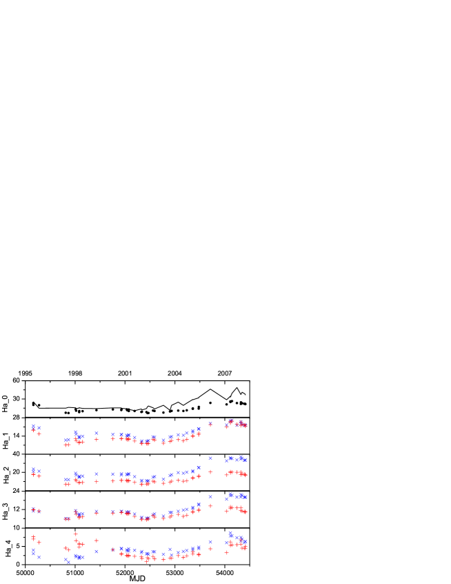
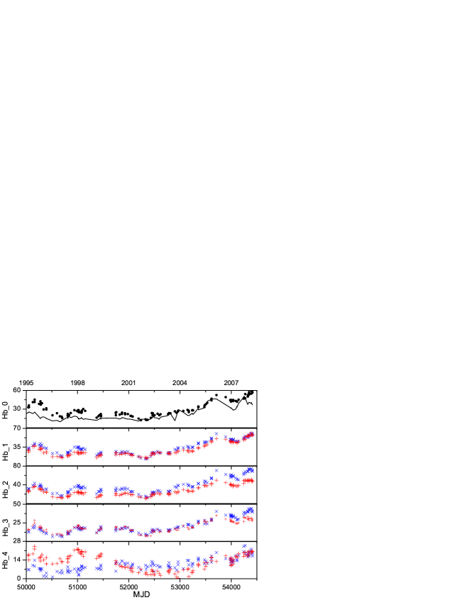
Figure 8: The light curves for different segments of the H$\alpha$ (top) and H$\beta$ (bottom) broad emission lines. The line-segment fluxes are given in $10^{-14}$ and $10^{-15}{\rm erg\leavevmode\nobreak\ cm^{-2}\leavevmode\nobreak\ s^{-1}}$ for H$\alpha$ and H$\beta$, respectively, while the date is given in the Modified Julian Date as MJD=JD-2400000.5 The mean velocity for segments number is as following: ($\pm$4) correspond ($\pm$8500)${\rm km\ s^{-1}}$ ; ($\pm$3) correspond ($\pm$6000); ($\pm$2) correspond ($\pm$4000); ($\pm$1) correspond ($\pm$2000)${\rm km\ s^{-1}}$; 0 corespond (1000)${\rm km\ s^{-1}}$. The blue part is denoted with crosses, the red part with pluses, and the line core with full circles. The solid line represents the continuum flux in arbitrary units for comparison.

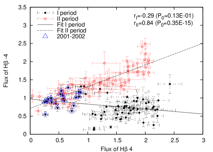
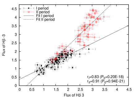
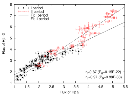
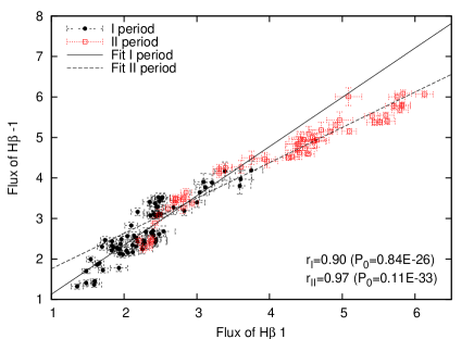
Figure 9: The line segment vs. line segment response. The observations in Period I are denoted with full circles and in Period II with open squares. The line-segment flux is in units $10^{-14}\,{\rm erg\,m^{-2}\,s^{-1}}$. The Pearson correlation coefficient $r$ and the null hypothesis value $P_{0}$ are given on each plot for both periods.

Table 2: The beginning and ending radial velocities, $V_{\rm beg}$ and $V_{\rm end}$, for different segments in the line profiles of H$\alpha$ and H$\beta$.

	-4	-3	-2	-1	0(C)	+1	+2	+3	+4
$V_{\rm beg}$	-10000	-7000	-5000	-3000	-1000	1000	3000	5000	7000
$V_{\rm end}$	-7000	-5000	-3000	-1000	1000	3000	5000	7000	10000

4.1 Line segment vs. line segment and continuum variations

We study the response of symmetrical line segments (-4 vs. 4, etc.), and as it shown in Fig. 9, there is only a weak response from the far blue to the far red segment in Period I. We plot the best linear fits for Period I and Period II, and find that the correlation between the far wings (segment -4 vs. segment +4) has a negative tendency with low significance (the Pearson correlation coefficient $r=-0.29$, the null hypothesis value $P_{0}$=0.13E-01), but in the Period II there is a linear response of the blue to the red wing with significant correlation ($r=0.84$, $P_{0}$=0.35E-15). In other segments, one can see that the change in the blue wing in Period I was smaller than in the red one (Fig. 9). It is interesting that in the Period I, the flux of the far blue wing (-4) stays nearly constant, while the flux of the red part (+4) is increasing. Even if we consider the Period I without the period 2001-2002, the correlation is weak and insignificant ($r=0.03$, $P_{0}$=0.84) and in favor of the previous statement.

To see whether there is a similar response of the line segments to the continuum flux we construct plots in Figs. 10 and 11 (Fig. 11 available electronically only), where the flux of all segments against the continuum flux are presented. As it can be seen in Figs. 10 and 11 there is a relatively good response of the line segments to the continuum flux (see plots for the values of the Pearson correlation coefficient $r$ and the null hypothesis $P_{0}$ for both periods). However, the line segments ($\pm$4) (especially in the case of the H$\beta$ line (Fig. 10, top)) in the Period I have a weak response (or even absent response, in the case segment +4) to the continuum flux. For example, the flux in the far red segment (H$\beta$ +4) increases around 4-5 times without the increase of the continuum flux.

Note here that in the H$\beta$ segment +4 one can expect higher errors due to the subtraction of the bright [OIII] lines. As a consistency check, we plot in Fig. 10 (bottom) H$\alpha$ ($\pm$4) segments fluxes vs. continuum flux. As it can be seen, the trend is similar as in H$\beta$, and also in Period I H$\alpha$ segment ($\pm$4) fluxes do not respond to the continuum flux. This may indicate that there are periods when some processes in the disk that are not connected with the central continuum source.

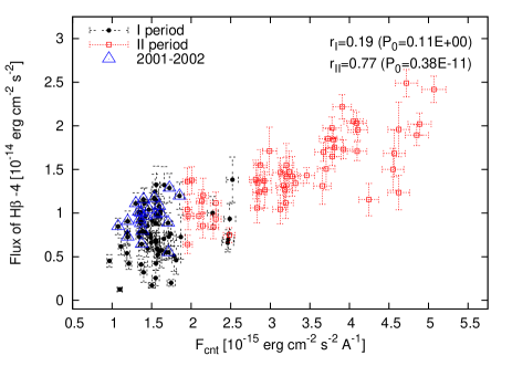
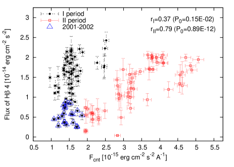
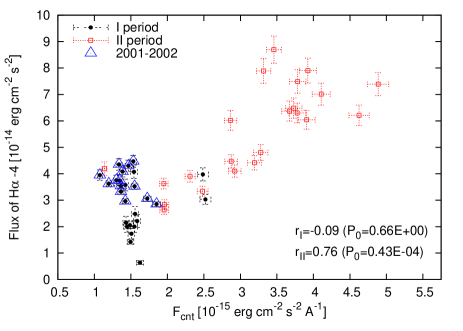
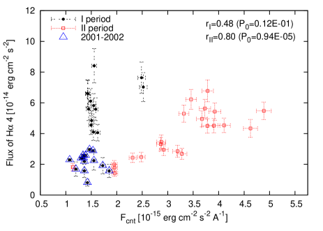
Figure 10: The far blue (left) and far red (right) wings flux against the continuum-flux variation for H$\beta$ (top) and H$\alpha$ (down). The notation is the same as in Fig. 9. The Pearson correlation coefficient $r$ and the null hypothesis value $P_{0}$ are given on each plot for both periods.

11

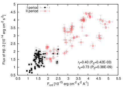
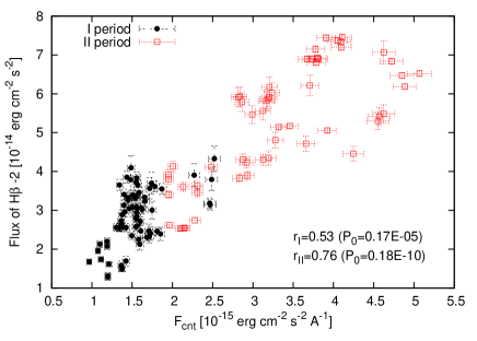
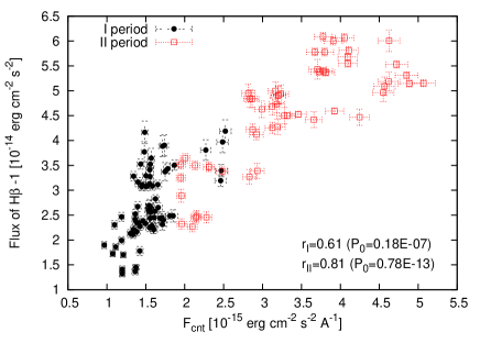
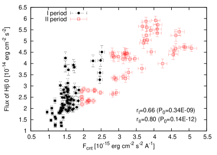
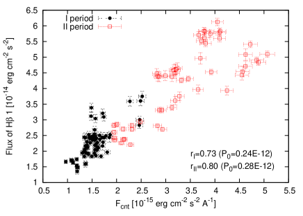
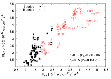
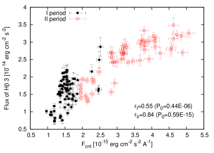
Figure 11: The same as in Fig. 10, but for the rest of line-segments: -3, -2, -1, 0, 1, 2, 3.

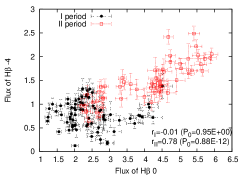
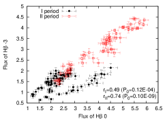
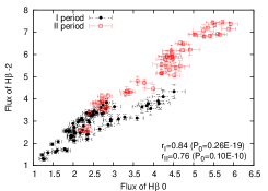
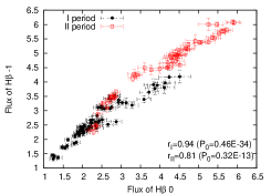
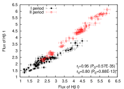
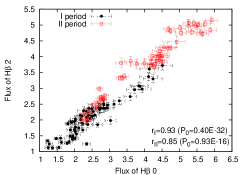
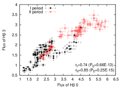
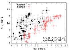
Figure 12: The response of the line segments to the central segment 0 (from -1000 to 1000 km s^-1). The observations in Period I are denoted with full circles and in Period II with open squares. The line-segment flux is in units $10^{-14}\,{\rm erg\,m^{-2}\,s^{-1}}$. The Pearson correlation coefficient $r$ and the null hypothesis value $P_{0}$ are given on each plot for both periods.

As mentioned above, there is a central peak that is probably coming from an additional emission region or is created due to some perturbation in the disk. Therefore we plot in Fig. 12 the line-segment fluxes vs. the flux of the central line-segment 0 (measured between -1000 and +1000 km s^-1). As it can be seen there is a good correlation between the central line-segment flux and fluxes of other segments, only one can conclude that the responses was better in the Period II. Thus, it seems that in this period both the disk-line and additional component effectively respond to the continuum variation. Also, one can see that the flux of the red part (segment +4) in Period I has a weak response to the central line-segment 0 ($r=0.58$, $P_{0}$=0.76E-07), that is similar as in the case of the segment to the continuum flux correlation (Fig. 10). This may have the same physical reason, that some kind of perturbation in disk were present in Period I.

4.2 Modeling of the line segment variation of the H$\beta$ line

We used the same models as described in §3.2, but now we have measured the line-segments fluxes for the modeled lines, defined in the same way as for the observed lines. Here we plot in Fig. 13 the sum of -4 and -3 segment fluxes as a function of the sum of +4 and +3 segment fluxes normalized on the central 0 segment, i.e. $F_{\rm blue\ wing}=[F(-4)+F(-3)]/F(0)$ vs. $F_{\rm red\ wing}=[F(+4)+F(+3)]/F(0)$.

Observations in Period I are denoted with full circles and in Period II with open squares (see Fig. 13). Also we see that observations in 2001 and 2002 are closer to the Period II, so we denoted these with open triangles. It is interesting that in the first period a good correlation between $F_{\rm blue\ wing}$ and $F_{\rm red\ wing}$ is present. The modeled $F_{\rm blue\ wing}$ vs. $F_{\rm red\ wing}$ relationship, marked with full triangles, appears to follow the trend of the observed points in Period I but is shifted below the observed correlation pattern. To find the causes for such disagreement, we measured the shift of the H$\beta$ averaged profiles for two periods (given in Paper I) with respect to the averaged profile constructed from the modeled profiles (for different positions of the H$\beta$ emitting disk). We measured the shift at the center of the width of the H$\beta$ line at half maximum and at 20% of the maximum. We found that the shift of the modeled average profile is +900 km s^-1 at 20% of the maximum and +600 km s^-1 at half maximum, while the measurements for Period I are $\sim$+700 km s^-1 at 20% of the maximum and $\sim$+110 km s^-1 at half maximum. In Period II the observed averaged H$\beta$ line was more blue-shifted with respect to the modeled one. We found $\sim$+310 km s^-1 at 20% of the maximum and $\sim$ -330 km s^-1 at half maximum. Therefore we simulated the segment variation (Fig. 13) taking into account that the whole disk line is blue-shifted by 300 km s^-1 (open circles in Fig. 13), and 850 km s^-1 (diamonds in Fig. 13). As can be seen in Fig. 13 the modeled values well fit the observations from Period I (line blue-shifted for 300 km s^-1) and Period II (line blue-shifted for 800 km s^-1). It is interesting that in Period I there are changes in the location of disk regions responsible for the lines emission (from R${}_{\rm inn}=250$ R_g to R${}_{\rm inn}=550$ R_g), while in Period II, the inner disk radius appears to have been changed by a smaller amount (from 350 R_g to 450 R_g). This indicates that in the first period (excluding 2001–2002) the variability can be well explained by variation of the disk position with respect to the black hole, while in the Period II and 2001–2002 (when outburst is starting), probably the disk position does not change so much. It seems that in this case we have that the part of the disk emitting the broad lines has only become brighter.

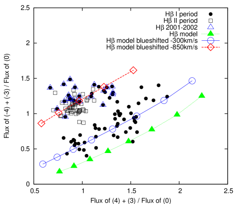
Figure 13: The ratio between the blue-wing flux (two blue segments, -4 and -3) and the central segment as a function of the ratio of the red-wing (two red segments, +4 and +3) and the central segment. Observations in Period I are denoted with full circles, in Period II with open squares, while observations from 2001–2002 are denoted with open triangles.

4.3 2-D CCF of the H$\beta$ line profiles

We now investigate in detail the cross correlation function (CCF) of the line-profile variations of H$\beta$. We proceed in the same way as it was studied the line-profile variations in Mrk 110 (, 2002, 2003).

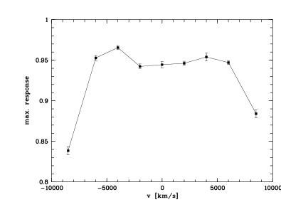
Figure 14: Maximum response of the correlation functions of the H$\beta$ line segment light curves with the continuum light curve.

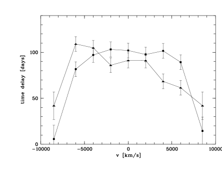
Figure 15: Time delay of the individual line segments of H$\beta$ for the first half of the observing period from 1995–2002 (filled squares) and for the second half from 2003–2007 (filled triangles) with respect to the continuum light curve in velocity space.

Fig. 14 shows the maximum response of the correlation functions of the H$\beta$ line segment light curves with the continuum light curve and Fig. 15 shows the delays of the individual H$\beta$ line segments in velocity space. Fig. 15 gives the delays of the individual line segments of H$\beta$ separately for the two observing periods: from 1995–2002 (filled squares) and from 2003–2007 (filled triangles).

The outer blue and red line wings show the shortest delay clearly indicating that the line emitting region is connected with an accretion disk (e.g. , 1991, 2004). A careful inspection of the delays of the individual line segments in Fig. 15 indicates that a second trend is superimposed: An earlier response of the red line wing compared to the blue line wing is seen in Fig. 15 for the second half of the observing period. This behavior is consistent with the prediction from disk-wind models (, 1994).

It is intriguing that the very-broad line AGN 3C 390.3 shows the same pattern in the velocity-delay maps as the narrow-line AGN Mrk 110 (see , 2002, 2003). The outer red and blue wings respond much faster to continuum variations than the central regions.

Figure 16: Variations in the continuum flux at 5100 Å  (first panel), in H$\alpha$ and H$\beta$ line fluxes (second and third panel, respectively), and in the integral Balmer decrement BD=$F(H\alpha)/F(H\beta)$ (fourth panel) of the month-averaged profiles. The abscissa (OX) gives the Modified Julian date (bottom) and the corresponding year (top). The continuum flux is in units $10^{-15}\,{\rm erg\,m^{-2}\,s^{-1}\,\AA^{-1}}$ and line flux is in $10^{-13}\,{\rm erg\,m^{-2}\,s^{-1}}$. The bottom panel gives the BD as a function of the continuum flux, where full circles denote the observations in Period I and open squares in Period II (see text).

5 Balmer Decrement (BD) variation

The ratio of H$\alpha$ and H$\beta$ depends on the physical processes in the BLR and variations in the Balmer decrement (BD) during monitoring time can indicate changes in physical properties of the BLR. Using the month-averaged profiles of the broad H$\alpha$ and H$\beta$ lines, we determined their integrated fluxes in the range between -10000 and +10000 ${\rm km\leavevmode\nobreak\ s^{-1}}$ in radial velocity, i.e. the integrated flux ratio $F(H\alpha)/F(H\beta)$ or integrated BD. In Fig. 16 we plot the time variation of the continuum flux, H$\alpha$ and H$\beta$ line fluxes and the BD. The BD reached its maximum in 2002 when the fluxes of lines and continuum were in the minimum. As one can see from Fig. 16 there is no correlation between BD and line/continuum variation. Only, as it can be seen in the very bottom panel in Fig. 16, which shows separate BDs for two periods (full circles represent Period I, and open squares Period II), there is some tendency that the BD is higher for weaker continuum flux. When BD is plotted versus the continuum flux (Fig.16 bottom panel) a negative trend seems to be present below 1.75 $\times 10^{-15}\rm erg\ cm^{-2}s^{-1}\AA^{-1}$. For higher values of the flux BD stays roughly constant. Note that a similar BD behavior was observed by (2010).

Figure 17: Variations in the Balmer decrement (BD=H$\alpha$/H$\beta$) as a function of the radial velocity for month-averaged spectra of 3C 390.3. Upper panel represents BD from the period of 1995–1998, and bottom panel from 2007. These two panels are chosen since they represent the characteristic behavior of BD vs. velocity. The abscissa (OX) indicates the radial velocities relative to the narrow components. The position of the blue, central and red peaks are marked with blue, black and pink line, respectively for H$\alpha$ (solid line) and H$\beta$ (dashed line). The rest of the panels are available electronically only.

17

Figure 18: Continued.

17

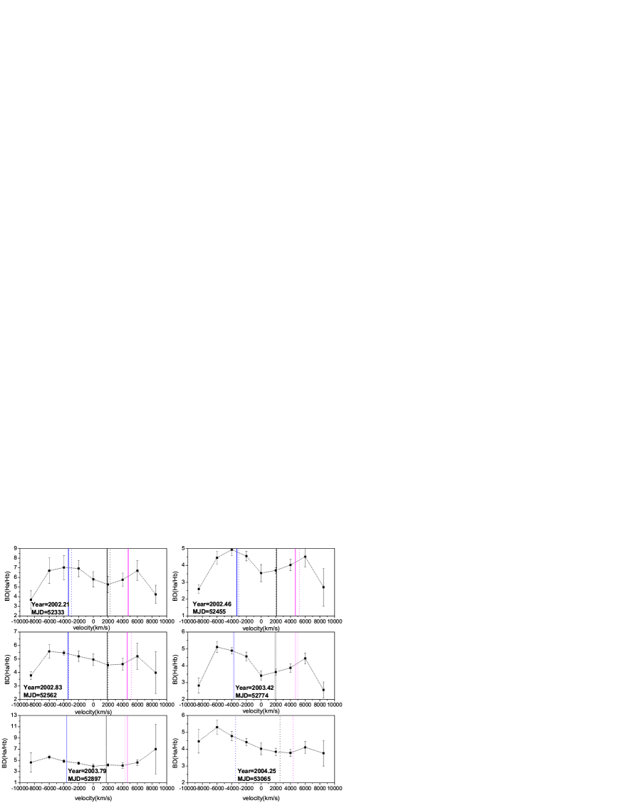
Figure 19: Continued.

17

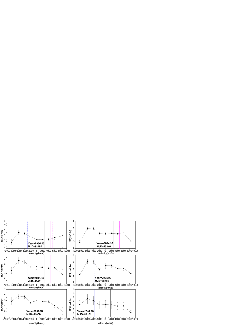
Figure 20: Continued.

5.1 BD as function of the velocity along line profile

Furthermore, we investigate BDs for each line segment (as it was described in §4), and plots of BD against velocity are present in Fig. 20 (note here that a part of this Figure is available electronically only). Fig. 20 shows some common features in the trends of the different line segments BD plotted vs. velocity over an extended period of time ranging from 1995 to 2007. For example, for almost all observations there is a minimum in the far blue and red wings (around $\pm$9000 km s^-1) as well as two maxima in red and blue part (around $\pm$6000 km s^-1). There is also a central minimum (around 0 km s^-1) that in 2001 and 2002 is moving to +2000 km s^-1, while in 2005 and 2006 is moving to -2000 km s^-1. It is interesting that from 2007 to the end of the monitoring period only a peak in the blue part (between -6000 to -4000 km s^-1) is dominant, while BD from -2000 to +6000 km s^-1 tends to be constant having values between 3.5 and 4.5.

3

Table 3: The errors of measurements ($e\pm\sigma$) for line segments of H$\alpha$ and H$\beta$ given in percent. For each segment the mean year flux is given in units $10^{-15}$ erg cm^-2 s^-1 Å^-1 for H$\beta$ and $10^{-14}$ erg cm^-2 s^-1 Å^-1 for H$\alpha$.

Year	Ha(-4)		Ha(+4)		Ha(-3)		Ha(+3)
	Flux	$(e\pm\sigma)$	Flux	($e\pm\sigma$)	Flux	($e\pm\sigma$)	Flux	($e\pm\sigma$)
1998	2.15	11.17$\pm$1.34	6.46	13.26$\pm$5.49	9.56	7.48$\pm$2.51	8.35	8.61$\pm$5.87
2001	4.18	5.04$\pm$3.26	2.71	2.89$\pm$1.54	10.48	2.00$\pm$2.30	9.73	1.62$\pm$0.03
2002	3.32	3.29$\pm$2.90	1.76	27.65$\pm$10.92	7.24	3.88$\pm$1.97	6.25	5.27$\pm$4.61
2004	4.03	5.67$\pm$0.65	2.71	12.70$\pm$1.87	12.47	3.25$\pm$0.66	9.16	5.22$\pm$2.65
2007	7.21	5.93$\pm$4.77	5.56	10.41$\pm$3.20	20.95	3.21$\pm$2.18	12.00	6.21$\pm$4.68
mean		6.22$\pm$2.96		13.38$\pm$8.99		3.96$\pm$2.08		5.39$\pm$2.51
Year	Hb(-4)		Hb(+4)		Hb(-3)		Hb(+3)
	Flux	($e\pm\sigma$)	Flux	($e\pm\sigma$)	Flux	($e\pm\sigma$)	Flux	($e\pm\sigma$)
1996	9.24	18.78$\pm$12.26	9.23	8.56$\pm$3.46	18.57	9.51$\pm$1.05	23.03	9.47$\pm$0.53
1998	6.72	35.15$\pm$21.79	20.29	4.79$\pm$0.14	18.21	8.16$\pm$3.46	19.20	7.76$\pm$2.90
2001	10.33	11.11$\pm$3.97	7.57	9.72$\pm$13.35	16.38	5.09$\pm$1.29	17.68	1.36$\pm$1.41
2002	9.94	12.98$\pm$8.09	4.94	19.88$\pm$9.73	13.38	10.40$\pm$4.84	12.09	12.82$\pm$3.51
2003	8.66	16.30$\pm$2.26	3.97	38.00$\pm$35.66	16.55	5.24$\pm$0.58	15.01	5.88$\pm$1.27
2004	12.87	11.33$\pm$7.25	7.46	29.39$\pm$31.57	24.06	5.94$\pm$3.74	21.25	4.41$\pm$3.17
2007	17.70	6.29$\pm$2.71	18.76	4.29$\pm$3.95	39.19	1.81$\pm$0.79	28.94	3.59$\pm$1.69
mean		15.99$\pm$9.34		16.37$\pm$13.13		6.59$\pm$2.97		6.47$\pm$3.87
Year	Ha(-2)		Ha(+2)		Ha(-1)		Ha(+1)		Ha(0)
	Flux	($e\pm\sigma$)	Flux	($e\pm\sigma$)	Flux	($e\pm\sigma$)	Flux	($e\pm\sigma$)	Flux	($e\pm\sigma$)
1998	16.61	6.14$\pm$2.69	10.09	6.32$\pm$4.90	14.67	5.61$\pm$2.20	10.19	8.03$\pm$4.36	10.69	11.76$\pm$2.78
2001	17.89	3.95$\pm$1.75	11.07	1.79$\pm$2.51	14.86	1.90$\pm$1.24	11.85	2.19$\pm$1.79	12.13	8.61$\pm$2.63
2002	12.18	3.03$\pm$1.24	8.07	2.36$\pm$2.37	11.08	3.51$\pm$2.66	9.32	2.12$\pm$1.16	8.94	6.21$\pm$4.95
2004	20.39	3.74$\pm$0.56	12.21	2.59$\pm$1.01	16.55	5.79$\pm$2.84	12.47	4.71$\pm$3.17	12.51	5.39$\pm$2.43
2007	34.96	2.17$\pm$2.34	18.78	5.48$\pm$4.22	24.08	1.78$\pm$1.85	23.40	4.66$\pm$3.02	23.51	4.11$\pm$3.25
mean		3.80$\pm$1.48		3.71$\pm$2.04		3.72$\pm$1.94		4.34$\pm$2.42		7.22$\pm$3.02
Year	Hb(-2)		Hb(+2)		Hb(-1)		Hb(+1)		Hb(0)
	Flux	($e\pm\sigma$)	Flux	($e\pm\sigma$)	Flux	($e\pm\sigma$)	Flux	($e\pm\sigma$)	Flux	($e\pm\sigma$)
1996	39.53	7.63$\pm$2.38	33.87	3.87$\pm$2.51	39.70	5.42$\pm$2.29	34.28	4.27$\pm$2.04	41.34	6.48$\pm$0.50
1998	35.39	3.93$\pm$2.28	23.30	5.86$\pm$2.25	32.53	2.88$\pm$2.99	24.02	4.15$\pm$3.05	26.53	5.28$\pm$0.93
2001	28.85	3.75$\pm$4.86	20.58	2.86$\pm$1.89	23.18	3.68$\pm$3.51	21.78	3.88$\pm$0.005	20.54	4.33$\pm$1.56
2002	21.70	7.15$\pm$5.92	17.42	5.60$\pm$ 4.49	20.89	5.03$\pm$2.52	20.94	6.28$\pm$4.36	18.96	7.55$\pm$0.75
2003	30.27	2.63$\pm$1.54	22.14	6.57$\pm$1.64	26.85	4.50$\pm$0.31	23.96	2.07$\pm$0.44	24.05	4.96$\pm$2.26
2004	39.90	3.24$\pm$3.11	29.87	2.53$\pm$2.26	38.13	2.59$\pm$1.31	30.37	2.66$\pm$1.70	30.41	3.44$\pm$2.36
2007	67.48	1.16$\pm$0.69	47.00	1.86$\pm$1.16	55.00	1.35$\pm$1.24	54.65	1.96$\pm$1.48	52.58	3.03$\pm$1.83
mean		4.21$\pm$2.36		4.16$\pm$1.85		3.64$\pm$1.46		3.61$\pm$1.52		5.01$\pm$1.61

4

Table 4: The line-segment fluxes for H$\alpha$ line in units $10^{-14}$ erg cm^-2 s^-1 Å^-1.

	MJD	Ha-4	Ha-3	Ha-2	Ha-1	Ha0	Ha1	Ha2	Ha3	Ha4
	(2400000+)	seg-4	seg-3	seg-2	seg-1	seg0 0	seg1	seg2	seg3	seg4
1	2	3	4	5	6	7	8	9	10	11
1	+50162.6	3.98	11.03	21.11	19.77	23.32	18.50	17.36	11.93	7.63
2	+50163.6	3.03	12.39	23.66	21.75	20.34	18.57	17.95	11.68	7.02
3	+50276.6	2.05	10.60	21.35	20.26	19.82	15.68	15.92	10.99	6.11
4	+50811.2	1.42	6.05	12.17	10.89	7.34	7.20	6.90	5.72	4.55
5	+50867.6	0.64	5.99	12.00	11.20	6.91	7.42	7.06	5.67	4.06
6	+51010.7	2.48	11.24	19.12	17.05	13.04	12.12	12.17	10.64	8.41
7	+51019.7	2.15	9.86	17.06	15.41	10.74	10.36	10.59	8.88	6.59
8	+51081.4	1.73	8.11	14.55	12.75	8.43	8.62	8.51	6.59	4.85
9	+51082.4	2.21	8.54	15.02	12.84	10.13	9.31	8.93	7.05	5.58
10	+51083.4	2.00	9.09	15.82	13.71	9.92	9.47	8.96	7.18	5.83
11	+51149.6	2.00	9.14	15.88	13.82	10.00	9.50	8.97	7.19	5.59
12	+51427.3	3.58	10.81	18.27	16.27	11.70	11.36	9.92	9.53	6.62
13	+51756.3	4.07	10.62	18.06	15.31	12.87	11.94	10.59	9.57	4.09
14	+51925.6	4.47	10.82	17.18	15.30	11.84	11.99	11.29	10.00	2.88
15	+51929.6	4.30	10.77	18.49	15.08	13.03	12.15	11.28	10.23	2.96
16	+52034.7	4.09	10.44	18.09	14.61	12.89	12.07	11.30	9.46	2.58
17	+52043.9	3.74	9.76	17.33	13.99	11.56	11.22	10.50	9.18	2.42
18	+52074.9	4.35	10.51	18.49	14.54	12.66	11.85	11.08	9.49	2.59
19	+52075.9	3.75	9.95	17.85	14.96	10.18	11.36	10.57	9.26	2.40
20	+52192.6	3.95	9.05	15.34	12.89	10.17	10.22	9.05	7.45	2.29
21	+52327.2	3.32	6.42	10.50	9.42	8.68	8.48	6.89	5.58	2.19
22	+52339.0	3.62	6.85	11.17	10.29	8.94	8.30	6.92	5.61	1.68
23	+52430.0	2.96	6.29	10.80	9.85	8.40	8.34	7.15	5.25	0.80
24	+52450.4	3.06	6.20	10.40	10.06	6.83	8.14	7.37	5.86	1.91
25	+52469.4	2.85	6.41	10.76	10.52	6.98	8.32	7.40	5.76	1.56
26	+52562.3	3.52	8.46	14.76	13.34	10.97	11.59	10.34	8.03	2.24
27	+52591.7	3.54	9.12	15.31	13.17	10.25	11.04	9.65	7.01	1.57
28	+52770.2	2.84	7.70	12.55	10.85	7.62	8.55	7.97	6.13	1.41
29	+52902.8	4.19	10.08	16.43	13.27	9.41	9.86	9.09	7.04	1.81
30	+52933.7	2.63	10.13	17.53	13.58	10.44	10.61	10.36	7.96	1.77
31	+53066.4	3.34	10.89	19.68	14.94	10.90	11.29	11.29	8.83	2.47
32	+53170.0	3.63	11.63	19.05	14.67	10.27	10.38	10.32	7.47	1.99
33	+53237.8	3.90	12.09	20.20	16.38	11.35	11.45	10.81	8.26	2.43
34	+53359.1	4.10	12.74	20.65	17.10	13.83	13.78	13.68	10.20	2.95
35	+53360.2	4.47	13.43	21.64	18.04	14.57	14.27	14.04	10.70	3.46
36	+53477.0	4.42	15.04	24.99	19.71	14.23	15.06	15.50	11.38	2.85
37	+53479.0	4.81	15.57	25.39	19.36	16.95	16.11	16.20	11.98	2.68
38	+53711.4	6.21	20.41	35.49	23.70	23.58	22.77	20.41	14.37	4.34
39	+54036.6	6.02	18.83	32.61	22.55	21.10	21.08	17.27	10.86	3.31
40	+54112.6	8.69	22.24	36.02	25.60	26.00	25.16	20.57	13.71	6.22
41	+54113.7	7.89	21.13	35.09	25.44	25.03	24.06	19.71	12.83	5.30
42	+54143.6	7.90	21.40	35.26	26.13	26.51	25.52	20.31	13.30	5.43
43	+54242.9	7.39	20.17	33.68	22.36	23.26	22.97	20.09	13.09	5.48
44	+54321.8	6.48	20.23	34.70	23.62	21.91	22.12	17.50	11.27	5.63
45	+54323.8	7.49	21.76	37.07	24.96	24.48	24.82	20.26	13.25	6.78
46	+54346.7	7.01	21.30	35.34	23.07	23.01	23.01	18.10	10.99	4.53
47	+54389.7	6.04	20.02	33.25	22.08	22.12	22.42	17.98	10.51	4.52
48	+54408.6	6.30	20.03	33.43	22.59	22.11	22.54	17.70	10.67	4.50
49	+54412.7	6.37	20.27	33.43	22.28	21.54	21.70	16.94	10.30	4.96

5

Table 5: The line-segment fluxes for H$\beta$ line in units $10^{-14}$ erg cm^-2 s^-1 Å^-1.

	MJD	Hb-4	Hb-3	Hb-2	Hb-1	Hb0	Hb1	Hb2	Hb3	Hb4
	(2400000+)	seg-4	seg-3	seg-2	seg-1	seg0	seg1	seg2	seg3	seg4
1	2	3	4	5	6	7	8	9	10	11
1	+49832.4	0.41	0.96	2.65	2.52	2.66	2.17	1.85	1.47	1.57
2	+49863.4	0.67	1.06	2.84	2.62	2.87	2.48	2.37	2.19	2.17
3	+50039.2	0.66	1.27	3.18	3.19	3.28	2.83	2.61	1.61	1.75
4	+50051.1	0.70	1.37	3.14	3.40	3.59	3.00	2.74	1.65	1.79
5	+50052.1	0.00	0.00	3.06	3.12	3.30	2.59	2.51	1.59	1.40
6	+50127.6	1.00	1.86	3.90	3.81	4.12	3.59	3.37	2.16	1.86
7	+50162.6	0.93	1.85	3.80	3.97	4.14	3.60	3.61	2.49	2.23
8	+50163.6	1.38	2.14	4.33	4.19	4.51	3.75	3.72	2.87	2.43
9	+50249.5	0.76	1.65	3.70	3.90	3.83	3.09	3.08	1.95	1.54
10	+50276.6	0.72	1.83	4.10	4.17	4.24	3.39	3.30	2.13	1.63
11	+50277.6	0.76	1.78	3.79	3.77	3.87	3.12	3.06	1.80	1.33
12	+50281.4	0.59	1.55	3.65	3.65	3.72	3.04	2.96	1.86	1.60
13	+50305.5	0.73	1.43	3.56	3.89	3.93	3.21	2.98	1.81	1.80
14	+50338.8	0.20	1.25	3.00	3.37	2.94	2.43	2.47	1.45	1.40
15	+50390.4	0.42	1.09	3.09	3.27	3.13	2.68	2.50	1.60	1.58
16	+50392.6	0.17	1.10	3.08	3.29	2.93	2.46	2.38	1.36	1.11
17	+50511.6	0.13	0.68	2.13	2.30	2.01	1.70	1.42	0.99	1.11
18	+50599.4	0.54	0.92	2.20	2.47	2.34	1.74	1.24	1.02	1.13
19	+50656.5	0.45	0.77	1.67	1.90	1.84	1.66	1.31	1.02	1.49
20	+50691.5	0.62	0.79	1.74	1.86	1.79	1.63	1.27	0.91	1.29
21	+50701.6	0.42	0.65	1.62	1.70	1.55	1.48	1.13	0.82	1.23
22	+50808.6	0.55	1.11	2.30	2.44	1.94	1.83	1.40	1.13	1.52
23	+50810.2	0.88	1.30	2.60	2.56	2.23	2.04	1.69	1.44	1.65
24	+50811.2	0.66	1.14	2.35	2.33	1.95	1.83	1.49	1.13	1.48
25	+50813.2	0.52	1.02	2.25	2.28	1.94	1.86	1.43	0.96	1.24
26	+50835.6	0.46	1.06	2.46	2.49	2.05	1.96	1.56	1.31	1.66
27	+50867.6	0.57	1.38	3.03	2.83	2.37	2.10	1.86	1.52	1.71
28	+50940.4	0.73	1.87	3.55	3.51	2.82	2.52	2.37	1.91	2.13
29	+50990.3	0.51	1.85	3.61	3.43	2.68	2.49	2.39	1.94	2.21
30	+51010.7	0.69	2.01	3.83	3.52	2.83	2.47	2.51	2.20	2.21
31	+51019.7	0.77	2.08	3.85	3.53	2.83	2.53	2.48	2.11	2.15
32	+51023.5	0.26	1.76	3.73	3.41	2.74	2.35	2.37	2.14	2.14
33	+51025.4	0.32	1.66	3.41	3.16	2.49	2.19	2.12	1.75	1.97
34	+51055.6	0.59	1.63	3.27	3.11	2.48	2.41	2.35	1.93	1.90
35	+51076.0	0.70	1.55	3.34	3.11	2.41	2.50	2.37	1.67	2.02
36	+51081.4	0.91	1.75	3.40	3.08	2.58	2.36	2.16	1.68	1.85
37	+51082.4	0.96	1.81	3.46	3.09	2.52	2.42	2.27	1.77	1.96
38	+51083.4	0.88	1.86	3.37	3.13	2.75	2.48	2.38	1.78	2.06
39	+51112.3	0.78	1.76	3.65	3.28	3.03	2.45	1.98	1.74	1.67
40	+51149.6	0.85	1.85	3.33	3.08	2.71	2.45	2.33	1.73	2.01
41	+51372.5	0.78	1.20	2.08	1.99	1.62	1.54	1.29	1.16	1.53
42	+51410.3	0.73	1.49	2.55	2.21	1.87	1.83	1.50	1.52	1.72
43	+51425.9	0.77	1.54	2.55	2.27	2.02	1.90	1.63	1.55	1.64
44	+51454.7	1.03	2.01	3.06	2.58	2.21	2.14	1.90	1.87	1.68
45	+51455.7	0.92	1.88	2.89	2.37	1.99	1.95	1.70	1.76	1.80
46	+51461.5	0.69	1.64	2.58	2.25	1.87	1.94	1.69	1.65	1.87
47	+51745.4	1.15	1.66	2.94	2.59	2.40	2.41	2.15	1.92	1.34
48	+51748.2	0.56	1.44	2.72	2.21	2.02	2.04	1.78	1.61	1.09
49	+51756.3	1.25	1.82	3.31	2.69	2.50	2.40	2.11	2.00	1.21
50	+51823.1	1.11	1.65	2.96	2.34	2.12	2.12	1.75	1.66	0.96
51	+51867.1	1.33	1.75	3.05	2.44	2.23	2.19	1.89	1.67	0.94
52	+51868.1	1.32	1.80	3.23	2.65	2.43	2.37	2.05	1.79	0.88
53	+51925.6	1.17	1.92	3.37	2.60	2.34	2.39	2.27	2.01	0.84
54	+51929.6	1.04	1.77	3.04	2.39	2.16	2.27	2.14	2.00	0.85
55	+51982.0	1.16	1.87	3.13	2.67	2.21	2.30	2.13	1.89	0.88
56	+52034.7	0.79	1.35	2.57	2.17	1.91	2.12	1.94	1.56	0.76
57	+52043.9	0.93	1.45	2.57	2.15	1.91	2.06	1.92	1.49	0.60
58	+52074.9	1.01	1.49	2.56	2.11	1.80	1.98	1.88	1.57	0.80
59	+52075.9	1.11	1.44	2.56	2.13	1.81	1.94	1.88	1.51	0.53
60	+52192.6	0.85	1.18	1.96	1.72	1.47	1.71	1.41	0.92	0.45
61	+52237.3	0.64	0.91	1.48	1.45	1.22	1.60	1.34	0.88	0.72
62	+52327.2	1.00	1.03	1.58	1.37	1.37	1.59	1.12	0.83	0.36
63	+52339.0	0.73	0.82	1.31	1.32	1.24	1.35	1.13	0.73	0.48
64	+52368.0	0.91	0.90	1.29	1.41	1.27	1.48	1.25	0.75	0.28
65	+52430.9	0.97	1.22	1.69	1.78	1.60	1.93	1.43	0.76	0.31
66	+52450.4	1.29	1.53	2.40	2.40	2.37	2.28	1.97	1.49	0.66
67	+52464.4	1.08	1.38	2.13	2.24	2.03	2.25	1.77	1.20	0.57
68	+52469.4	1.20	1.62	2.39	2.48	2.34	2.44	2.08	1.52	0.54
69	+52495.3	0.55	1.34	2.33	2.31	1.99	2.16	1.95	1.38	0.26
70	+52502.8	1.00	1.55	2.47	2.45	2.02	2.27	1.99	1.37	0.36
71	+52562.3	0.98	1.66	2.79	2.68	2.25	2.54	2.29	1.61	0.58
72	+52593.7	0.88	1.50	2.73	2.42	2.02	2.43	2.03	1.28	0.37
73	+52620.4	0.89	1.43	2.47	2.45	2.17	2.44	2.02	1.35	0.25
74	+52768.2	0.97	1.55	2.62	2.32	2.18	2.35	2.07	1.40	0.56
75	+52783.0	0.97	1.55	2.53	2.27	2.29	2.26	2.20	1.46	0.60
76	+52784.0	1.20	1.52	2.55	2.48	2.36	2.39	1.94	1.29	0.57
77	+52786.0	0.85	1.40	2.54	2.45	2.33	2.37	2.00	1.36	0.44
78	+52813.0	0.84	1.59	2.74	2.46	2.33	2.21	2.02	1.51	0.70
79	+52900.8	0.83	1.73	3.59	3.09	2.64	2.48	2.51	1.70	0.36
80	+52933.7	0.64	1.88	3.40	2.89	2.40	2.42	2.25	1.55	0.14
81	+52962.6	1.06	1.89	3.83	3.27	2.64	2.81	2.41	1.57	0.04
82	+52963.6	1.26	1.99	3.90	3.39	2.70	2.70	2.59	1.82	0.49
83	+53065.5	0.75	2.05	4.12	3.38	2.71	2.94	2.99	2.15	0.66
84	+53146.0	1.38	2.29	4.13	3.65	2.87	2.85	2.77	1.93	0.70
85	+53169.0	1.36	2.31	3.92	3.52	2.76	2.82	2.72	1.77	0.74
86	+53171.9	1.04	2.22	3.80	3.25	2.52	2.60	2.47	1.65	0.16
87	+53236.8	0.93	1.89	3.46	3.47	2.79	2.82	2.68	1.93	0.43
88	+53238.9	1.12	2.13	3.63	3.47	2.82	2.70	2.64	1.86	0.49
89	+53254.8	1.14	2.02	3.61	3.50	2.80	2.71	2.65	1.91	0.61
90	+53358.1	1.47	2.71	4.30	4.25	3.42	3.39	3.38	2.51	1.11
91	+53359.1	1.37	2.58	4.23	4.12	3.30	3.31	3.33	2.42	1.03
92	+53360.2	1.55	2.74	4.31	4.22	3.37	3.31	3.33	2.42	0.96
93	+53476.0	1.12	2.36	4.35	4.27	3.33	3.61	3.80	2.66	0.72
94	+53479.0	1.42	2.85	4.81	4.50	3.60	3.75	3.86	2.83	1.21
95	+53504.0	1.31	2.59	4.71	4.42	3.78	3.97	3.77	2.48	0.94
96	+53531.9	1.15	2.37	4.46	4.47	4.00	3.93	3.80	2.68	1.20
97	+53612.8	1.68	3.00	5.41	5.09	4.55	4.54	4.29	2.84	1.56
98	+53613.8	1.50	2.89	5.30	4.96	4.40	4.43	4.07	2.78	1.34
99	+53614.8	1.24	2.83	5.49	5.19	4.67	4.71	4.29	3.10	1.63
100	+53711.4	1.96	4.03	7.07	6.01	5.25	5.09	4.98	3.49	1.29
101	+53891.5	1.51	3.54	6.21	5.43	4.92	4.96	4.47	3.02	1.72
102	+53979.8	1.47	3.58	6.03	4.94	4.45	4.65	4.19	2.92	1.48
103	+53994.8	1.04	3.27	5.56	4.69	4.20	4.38	3.92	2.71	1.03
104	+53995.8	1.31	3.38	5.82	5.00	4.49	4.59	4.03	2.80	1.57
105	+53996.7	1.55	3.46	5.91	4.91	4.33	4.60	4.01	2.70	1.37
106	+53997.7	1.42	3.58	6.17	4.92	4.44	4.62	4.02	2.89	1.22
107	+53998.8	1.27	3.46	5.86	4.73	4.42	4.49	3.89	2.66	0.99
108	+54036.6	1.24	3.27	5.79	4.83	4.29	4.37	3.66	2.68	1.08
109	+54037.6	1.38	3.49	5.91	4.95	4.47	4.47	3.96	2.70	1.44
110	+54040.7	1.35	3.36	5.93	4.84	4.35	4.40	3.87	2.58	1.29
111	+54088.2	1.71	3.23	5.46	4.63	4.31	4.41	3.77	2.44	1.70
112	+54112.6	1.43	2.94	5.17	4.53	4.22	4.31	3.75	2.46	1.65
113	+54113.7	1.34	2.89	5.14	4.50	4.19	4.26	3.74	2.42	1.59
114	+54143.6	1.73	3.01	5.05	4.59	4.52	4.53	3.83	2.52	1.88
115	+54242.9	2.02	3.53	6.19	5.15	4.73	4.83	4.28	2.70	1.68
116	+54243.9	2.42	3.88	6.52	5.15	4.68	5.10	4.88	3.26	1.95
117	+54271.9	1.89	3.73	6.47	5.31	4.74	4.91	4.81	3.17	1.79
118	+54273.0	2.49	3.93	6.84	5.53	5.41	5.41	5.07	3.22	2.00
119	+54321.8	1.85	4.01	6.90	5.38	5.02	5.52	4.90	3.06	1.70
120	+54323.8	1.65	3.93	6.81	5.40	5.26	5.62	5.07	3.33	1.97
121	+54324.8	1.75	4.04	6.90	5.37	5.05	5.44	4.75	2.99	1.70
122	+54346.7	1.96	4.24	7.46	5.81	5.72	5.82	5.04	3.11	1.86
123	+54347.7	2.03	4.42	7.34	5.68	5.53	5.79	5.00	3.02	2.06
124	+54348.7	1.71	4.17	7.20	5.55	5.35	5.60	4.79	2.86	1.86
125	+54389.7	2.22	4.43	7.44	6.00	5.48	5.75	4.95	3.04	2.00
126	+54391.6	2.05	4.36	7.38	6.07	5.92	6.13	5.16	3.17	1.99
127	+54406.7	1.84	3.98	6.92	5.78	5.61	5.82	4.77	2.78	2.00
128	+54408.6	1.98	4.14	7.15	6.09	5.88	5.84	4.84	2.90	2.04
129	+54412.7	1.70	3.98	6.89	5.78	5.66	5.71	4.71	2.95	2.06

Table 5: Continued.

Figure 21: The Balmer decrement versus velocity. First two panels – the inner radius is the same, but different positions of the H$\alpha$ and H$\beta$ disk with respect to the black hole are assumed. The bottom panel shows the cases where the one of the two emitting regions is closer to the central black hole. The inner and outer radii assumed in models are labeled on each panel. The BD points are normalized to the one at -4000 km s^-1.

5.2 Modeling of the Balmer decrement

It is known that the BD depends on physical processes. But BD as function of the velocities along the line profile may also depend on the geometry of the H$\alpha$ and H$\beta$ emitting region, as e.g. if the line emission region of H$\alpha$ and H$\beta$ are not the same one may expect that the H$\alpha$ and H$\beta$ flux ratio will be a function of the gas velocity. Therefore, we modeled the shape of the BD vs. velocity.

In order to test the influence of the geometry to the BD vs. velocity along the line, we used modeled disk profiles (see §3.2), but now we consider two cases: a) the disk regions emitting H$\alpha$ and H$\beta$ have different sizes but the same inner radii that vary accordingly (as discussed in §3.2); b) the inner radius of the H$\alpha$ emitting region differ from the fixed radius of the H$\beta$ region by $\pm 50R_{\rm g},\pm 100R_{\rm g}$.

Our simulations of the BD vs. velocity are given in Fig. 21, where it can be seen that the disk model (assuming different dimensions of the emission disk that emits H$\alpha$ and H$\beta$) can reproduce very similar BD profiles along velocity field, especially as they are observed in Period I. There is a difference in shape that is probably caused by the physical conditions in the disk as well as due to the central component emission. We found bell-like profiles of BD, and they also have two peaks (in red and blue part), as well as a small minimum in the center. The shape of the BD vs. velocity observed in Period II, where a peak in the blue part is prominent (see Fig. 20), and in some cases has a deeper red minimum than blue one, cannot be obtained in modeled BD vs. velocity. This may be due to the influence of the central component, but also, due to the outburst in Period II, or due to different physical processes in the disk.

As it can be seen in Fig. 21 (bottom panel, open squares), a big difference between modeled BD vs. velocity and observed one is in the case where the H$\alpha$ emitting region is closer to the black hole for 100 R_g. This indicates that the disk part emitting H$\alpha$ cannot to be significantly closer to the central black hole than the one that emits the H$\beta$ line.

6 Discussion

In this paper we performed detailed study of the line parameter variations (peak separation, variation of the line segments, Balmer decrement) during a 13-year long period. As we noted above, the line profiles of the 3C 390.3 in the monitoring period have a disk-like shape, i.e. there are mainly two peaks, where the blue one is more enhanced. In some periods, there is a central peak, that probably is coming from an additional emission region or extra emission caused by some perturbation in the disk (see e.g. , 2010). In order to confirm the disk emission hypothesis we modeled the peak position variation using a semi-relativistic model, and found that peak position variations can be explained with the disk model.

We also investigated line-segment flux variation and found that the ratios of the line segments are well fitted by a disk model. It is interesting that the response of the line-segment flux to line-segment flux is better in Period II than in Period I. The same is in the case of the response of the segment fluxes to the continuum flux. It seems that in Period I, the variability in the line profile was not caused only by an outburst in the ionizing continuum, but also by some perturbations in the accretion disk (see e.g. , 2010). While in Period II, it could be that the disk structure is not changing much and that the variability in the line parameters is primarily caused by the outburst in the continuum.

The Balmer decrement as a function of the continuum has a decreasing trend in Period I (with the increase of the continuum) and is constant in Period II. Also, there is a different shape of the BD vs. velocity in different periods. The characteristic shape of the BD vs. velocity has two peaks (blue and red) which do not correspond to the line peaks (they are in the far wings, see Fig. 20), there are minima in the far blue and red wing, as well as a minimum in the center. The shape of the BD vs. velocity is similar to what we expect from an accretion disk, where the dimensions of the disk for H$\alpha$ and H$\beta$ are different. In the period (Period II) of the highest brighteners in the continuum and in lines, the BD vs. velocity shapes show a blue peak and more-less flat red part, that is probably caused by some other emission, additional to the disk one, and also by different physical conditions in these two sub-regions. Our modeled shapes of the BD vs. velocity show that the case of the disk emission where the dimensions of the H$\alpha$ and H$\beta$ emitting disks are different, can explain bell-like shapes of the BD vs. velocity. Note here that we did not consider physical processes in the emitting disk which can affect the shape of the BD vs. velocity. Comparing the dimensions of the disk, we came to the same conclusion as from the CCF (see Paper I), that the H$\alpha$ emitting disk is larger than the H$\beta$ one, but also that the inner radius of both disks seems to be similar.

6.1 Variability and the BLR structure of 3C 390.3

Before we discuss the BLR structure, let us recall some results that we obtained in Paper I and in this paper: i) the CCF analysis shows that the dimension of the BLR that emits H$\beta$ is smaller than one that emits H$\alpha$; ii) there is a possibility that there are quasi-periodic oscillations, which may be connected with the instability in the disk or disk-like emitting region; iii) concerning the line profile variations, the variability observed in 13-year period can be divided into two periods, before and after the outburst in 2002; iv) there are three peaks, two which are expected in the disk emission, and one - central, that is probably coming from disk perturbations or from an additional emitting region; v) the shapes of H$\beta$ and H$\alpha$ observed in the same period are similar, especially in Period I (note here that in Period II, there are differences in the center and red wings); vi) our simulation of the variability, taking into account only different disk position with respect to the central black hole, can qualitatively explain the observed broad line parameter variations; vii) comparing the shifts of the modeled and observed H$\beta$ line, we found that there is a blue-shift in the observed H$\beta$ comparing to the modeled one, that is also different in two periods: around 300 km s^-1 in Period I and around 850 km s^-1 in Period II; viii) the inspection of the delays of the individual line segments (see §4.3) indicates presence of a disk and also a wind, i.e. the disk-wind model may be present in the BLR of 3C 390.3.

Additionally, note here that the disk-like structure of the 3C 390.3 BLR is favored in several recent papers (see e.g. , 2008, 2010) assuming an elliptical disk (, 2008) or perturbations in the disk (, 2010).

Taking into account all mentioned above, one can speculate about the BLR structure and the nature of these variations. Let us consider that, in principle, there is an accreting material that is optically thick, and the light from a central source is able to photoionize only a small thin region above (below) the accreting material (or thick disk, see Fig. 22), let us call this region a “disk-like broad line region” (disk-like BLR1). Emitting gas in this region has disk-like motion, since it is located in the disk periphery and follows the disk kinematics. The brightness of broad lines which are coming from this region will be caused by the central ionizing continuum source, but the line parameters will depend on the dimensions of the region as well as the location of the BLR1 with respect to the central black hole. Of course, other parameters as e.g. emissivity or local velocity dispersion can slightly affect the line profiles, but it seems that the change in the inner/outer radius is the most important.

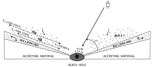
Figure 22: The model of the BLR that is composed of the disk-like BLR1, and an outflowing/inflowing BLR2.

The shape of the broad lines confirm the disk-like geometry, and correlation between the broad-line and continuum fluxes confirms the influence of the central source to the line intensity (see Paper I). The optical continuum and the H$\beta$ flux variations are probably related to changes in the X-ray emission modulated by variable accretion rate, i.e. the change of the surface temperature of the disk as a result of the variable X-ray irradiation (2000). But question is, what can cause the changes in the dimension (as well in position) of the broad line emitting region? It is obvious that it is not the continuum flux, since the variation in the continuum does not correlate with the line parameter variation.

The variation in the line parameters may be related to the perturbations in the accreting material that is feeding the disk-like BLR with scattered gas. The density and optical depth of such gas from the accreting material may cause that in different epochs the disk-like BLR has different dimensions and positions with respect to the central black holes. As, e.g. if scattered material (gas) from accreting material is absent in some parts, it will affect the line parameters similar as change in the dimensions (position) of the disk-like BLR.

On the other side, the observed broad double-peaked lines have a blue-shift with respect to the modeled one. This may indicate that there is some kind of wind in the disk, probably caused by the radiation of the central source. Recently (2010) performed an uniform and systematic search for the blueshifted Fe K$\alpha$ absorption lines in the X-ray spectra of 3C 390.3 observed with Suzaku and detected absorption lines at energies greater than 7 keV. That implies the origin of the Fe K$\alpha$ is in the highly ionized gas outflowing with mildly relativistic velocities (in the velocity range from 0.04 to 0.15 light speed). Taking into account that the optical line emission is probably originating farther away than the X-ray, one can expect significantly smaller outflow velocities in the optical lines.

One can expect that perturbations in the thick disk (or accreting material) can affect the emitting disk-like region. It may cause some perturbation or spiral shocks in the disk-like BLR (see e.g. , 1994, 2010). (1994) found that the observed variability of the double-peaked broad emission lines (seen in some active galactic nuclei) can be due to the existence of two-armed spiral shocks in the accretion disk. Using this model they successfully fitted the observations of 3C 390.3 made at different epochs with self-similar spiral shock models which incorporate relativistic corrections.

Alternatively, (2010) fitted the observations of 3C 390.3 from different epochs with a model that includes moving perturbation across the disk. The perturbations/shocks in the disk model can explain different line profiles, and also the central peak (see e.g. , 2010). But the central peak might be emitted from a broad line region that does not follow the disk geometry, it may be very similar to the two-component model, i.e. that we have composite emission from the disk and an additional region (see e.g. , 2004, 2006, 2009). Also, (2010) considered that the BLR of 3C390.3 has a complex structure composed from two components: 1) BLR1 – the traditional BLR (Accretion Disk), 2) BLR2 – a sub-region (outflow) that surrounds the compact radio jet. In this paper the existence of a jet-excited outflowing BLR is suggested, which may question the general assumption of a virialized BLR.

It is interesting that the central component is present during the whole monitoring period, and that in 1995–1996 it was located in the center, and after that shifted to the the red part of line. Such redshift is not expected if there is an outflow in the BLR. But let us recall the results obtained in the study of dynamics of the line-driven disk-wind, where kinematics of the gas shows that both infall and outflow can occur in different regions of the wind at the same time (see , 1998, 2000), which depends on radiation force. Also, recently (2009) reported about the possibility that an inflow is present in the BLR of AGN.

Finally, one can consider a model as given in Fig. 22: the disk-like BLR1 follows the kinematics of the accreting material, and from time to time perturbations can appear in this region (similar as in the fully accretion disk). The emitting gas in the BLR1 is coming (ejected) from the accreting material and it is ionized by the central source. The radiation pressure may contribute in such way that we have a wind (an outflow) in this region. There may be also a region above the disk-like BLR1 (a BLR2 in Fig. 22), where the ionized gas may have motion with respect to the central black hole, and depending on the radiation pressure the velocities are different in different periods.

6.2 Different nature of variation in broad lines of 3C 390.3

It is interesting to discuss the difference between the variation in Period I and Period II. It is obvious that the disk-parameters variation can explain the observed line-parameter variations (as e.g. in the peak separation and line-segment fluxes variations). In Period I, there were several quasi-periodical low-intensity outbursts (see Paper I), and it seems that the line, and consequently the disk-like geometrical parameters are changed. It may be that in this period the outbursts are caused by some perturbations in the disk (in the inner part that emits the X-ray radiation as well as in the outer part emitting the broad lines). These perturbations affected the line profiles and probably partly line fluxes (especially in the far wings). As it can be seen from modeled variation the inner/outer radius is significantly changed.

In the Period II, there is a strong outburst, that caused the increase of the brightness in the continuum and lines. The lines stay brighter, but the structure (inner/outer radius) of the disk-like region is not changing much. There is a different response of the continuum to the line segments in Period I and Period II, i.e. in Period II there is a higher correlations between the continuum and line-segment fluxes.

On the other hand, the BD in Period I has a decreasing trend with the increase of the continuum flux, while in Period II, it stays almost constant. This may indicate different nature of the variability. It seems that in Period I, beside the ionizing continuum influence on the line intensities (especially in the far wings), there was the additional effect that influence the line profiles and intensities. Probably it was caused by some perturbations or shocks in the disk-like BLR (, 1994, 2010) that produced changes in the structure of the disk-like BLR.

7 Conclusions

In this paper, we present line profile variations of 3C 390.3 in a long period. Due to the change of line profiles, we divided the observations into two periods (before and after the minimum in 2002: Period I and II, respectively) and found difference in the line segments and Balmer decrement variations in these two periods. From our investigation, the main conclusions are the following:

i) the line profiles during the monitoring period are changing, always showing the disk-like profile, with the higher blue peak. There is also the central peak that may come from the emission region additional to the disk, but as it was mentioned in (2010), it may also be caused by the perturbation in the disk.

ii) the far-wings flux variation in the first period, where the far-red wing flux does not respond well to the continuum flux, is probably caused by some physical processes in the innermost part of the disk. The observed changes in H$\alpha$ and H$\beta$ may be interpreted in the framework of a disk model with changes in the location and size of the disk line emitting regions. In Period II, the good correlation between the continuum and line-segment flux suggests that the brightness of the disk is connected with the ionizing continuum, and that the structure of the disk does not significantly change.

iii) Balmer decrement is also different for these two periods. In the first period the BD decreases with continuum flux, while in the second period the BD stays more-less constant (around 4.5). The segment BD shows two maxima (around $\pm$6000 km s^-1) which do not correspond to the red and blue peak, but instead they are farther in the blue and red wing (than peaks velocities). Also one minimum around zero velocity is present. This minimum changed position between $\pm$2000 km s^-1 around zero velocity. This central minimum (as well as shifted maxima) may be caused by the additional (to the accretion disk) emission that perhaps is present in the 3C 390.3 broad lines. These results suggest that, in addition to the physical conditions across disk, the size of the H$\alpha$ and H$\beta$ emitting regions of the disk plays an important role. We modeled bell-like BD vs. velocity profiles in the case when the H$\alpha$ disk is larger than H$\beta$ one.

iv) the variation observed in the line parameters can be well modeled if one assumes changes in position of the emitting disk with respect to the central black hole. The emission of the disk-like region is dominant, but there is the indication of the additional emission. Therefore, to explain the complex line-profile variability one should consider a complex model that may have a disk geometry together with outflows/inflows (see Fig. 22).

An important conclusion of this work is that, even if the disk-like geometry plays a dominant role, the variability of the H$\alpha$ and H$\beta$ line profiles and intensities (and probably partly in the continuum flux) has different nature for different periods. It seems that in Period I, the perturbation(s) in the disk caused (at least partly) the line and continuum amplification, while in Period II the ionizing continuum caused the line amplification without big changes in the disk-like structure.

References

- (1) Arshakian, T. G., León-Tavares, J., Lobanov, A. P., Chavushyan, V. H., Shapovalova, A. I., Burenkov, A. N., Zensus, J. A. 2010, MNRAS, 401, 1231
- (2) Bon, E., Popović, L. Č., Gavrilović, N., La Mura, G., Mediavilla, E. 2009, MNRAS, 400, 924
- (3) Chakrabarti, S. K., Wiita, P. J. 1994, ApJ, 434, 518 ch94
- (4) Chen, K., & Halpern, J. P. 1989, ApJ, 344, 115
- (5) Chen, K., Halpern, J. P. & Filippenko, A. V. 1989, ApJ, 339, 742
- (6) Dietrich, M., Peterson, B. M., Albrecht, P. et al. 1988, ApJS, 115, 185
- (7) Eracleous, M., et al. 1997, ApJ, 490, 216
- (8) Eracleous, M. & Halpern, J. P. 1994, ApJS, 90, 1
- (9) Eracleous, M. & Halpern, J. P. 2004, ApJS, 150, 181
- (10) Eracleous, M., Lewis, K. T., Flohic, H. M. L. G. 2009, NewAR, 53, 133
- (11) Flohic, H. M. L. G., & Eracleous, M. 2008, ApJ, 686, 138
- (12) Horne, K., Peterson, B. M., Collier, S. J., Netzer, H. 2004, PASP, 116, 465
- (13) Gaskell, C.M. 1996, ApJ, 464, L107
- (14) Gaskell, C. M. 2009, NewAR, 53, 140
- (15) Ilić, D., Popović, L. Č., Bon, E., Mediavilla, E. G., Chavushyan, V. H. 2006, MNRAS, 371, 1610
- (16) Jovanović, P., Popović, L. Č., Stalevski, M., Shapovalova, A. I. 2010, ApJ, 718, 168
- (17) Kollatschny, W. 2003, A&A, 407, 461
- (18) Kollatschny, W., & Bischoff, K. 2002, A&A, 386, L19
- (19) Königl, A., Kartje, J. F. 1994, ApJ, 434, 446
- (20) Lewis, K. T., Eracleous, M., Storchi-Bergmann, T. 2010, ApJS, 187, 416
- (21) Perez, E., Mediavilla, E., Penston, M. V., Tadhunter, C., Moles, M. 1988, MNRAS, 230, 353
- (22) Popović, L.Č., Mediavilla, E.; Bon, E.; Ilić, D. 2004, A&A, 423, 909
- (23) Proga, D., Stone, J. M., Drew, J. E. 1998 MNRAS, 295, 595
- (24) Proga, Daniel; Stone, James M.; Kallman, Timothy R. 2000, ApJ, 543, 686
- (25) Sergeev, S. G., Pronik, V. I., Peterson, B. M., Sergeeva, E. A., Zheng, W. 2002 ApJ, 576, 660
- (26) Sergeev, S. G., Klimanov, S. A., Doroshenko, V. T., Efimov, Yu. S., Nazarov, S. V., Pronik, V. I. 2010 MNRAS, tmp.1496S
- (27) Shapovalova, A.I., Burenkov, A.N. , et al., 2001, A&A, 376, 775
- (28) Shapovalova, A. I., Doroshenko, V. T., Bochkarev, N. G., et al. 2004, A&A, 422, 925
- (29) Shapovalova, A. I., Popović, L. Č., Burenkov, A. N. et al. 2010, A&A, 517A, 42
- (30) Sulentic, J. W., Marziani, P., Dultzin-Hacyan, D. 2000, ARA&A, 38, 521
- (31) Tombesi, F., Sambruna, R. M., Reeves, J. N., Braito, V., Ballo, L., Gofford, J., Cappi, M., Mushotzky, R. F. 2010, ApJ, 719, 700
- (32) Ulrich, M.-H. 2000, A&A Rev., 10, 135
- (33) Van Groningen, E., & Wanders, I.1992, PASP, 104, 700
- (34) Veilleux, S. & Zheng, W. 1991, ApJ, 377, 89.
- (35) Welsh, W. F., Horne, K. 1991, ApJ, 379, 586
- (36) Zamfir, S., Sulentic, J. W., Marziani, P., Dultzin, D. 2010, MNRAS, 403, 1759
- (37) Zheng, W. 1996, AJ, 111, 1498