Optical realization of the two-site Bose-Hubbard model in waveguide lattices

Abstract

A classical realization of the two-site Bose-Hubbard Hamiltonian, based on light transport in engineered optical waveguide lattices, is theoretically proposed. The optical lattice enables a direct visualization of the Bose-Hubbard dynamics in Fock space.

The Bose-Hubbard Hamiltonian provides a paradigmatic theoretical framework to investigate the physics of strongly interacting bosonic systems [1]. In particular, the two-site Bose-Hubbard model has received a great deal of attention in the last decade as a simple model to investigate the dynamics of ultracold bosonic atoms confined in a double-well potential [2, 3, 4, 5, 6, 7, 8], the so-called bosonic junction (for a recent review see [9]). A remarkable property of the bosonic junction is the existence of Josephson-like oscillations of the atomic populations and of macroscopic self trapping due to atom-atom interaction, which were originally predicted within a semiclassical (mean-field) limit of the Bose-Hubbard model [2, 3]. However, various quantum features of the Bose-Hubbard dynamics, such as quantum fluctuations, fragmentation [10], the cat-states formation in the supercritical attractive case [11], or the many-body coherent control of tunneling [12, 13], are not accessible within the mean-field limit. This has lead to intensive studies on the relation between the full quantum and mean-field dynamics (see, e.g., [14, 15, 16, 17] and references therein). A comprehensive description of the entire variety of phenomena rooted in the Bose-Hubbard Hamiltonian would benefit from a direct access to quantum dynamical evolution in the Fock space. However, in experiments with ultracold gases the measurable quantities are usually atomic population imbalance and relative phases [3], whereas full information on Fock state occupation evolution is generally not accessible.

In another physical context, light transport in waveguide lattices has provided a test bench to visualize in photonic systems the classical analogues of a wide variety of coherent single-particle quantum phenomena generally encountered in condensed matter or matter wave systems [18, 19, 20], such as Bloch oscillations and Zener tunneling [18, 21], dynamic localization [22, 23], and Anderson localization [24, 25] to mention a few. As compared to quantum systems, photonic lattices enable a direct and complete visualization of the dynamics by mapping the temporal evolution of the quantum system into spatial propagation of light waves in the engineered lattice [19]. Most of such previous quantum-optical analogue studies, however, focused on single-particle effects, whereas the possibility to visualize in a classical optical setting the analogues of many-particle phenomena, such as those rooted in the Bose-Hubbard model, remains unexplored. Recently, photonic lattices with engineered coupling constants have been proposed as classical analogs to quantum coherent and displaced Fock states [26].

In this Letter it is shown that photonic lattices with suitably engineered coupling and propagation constants provide a simple realization in the Fock space of two-site Bose-Hubbard Hamiltonian.

The starting point of the analysis is provided by a standard two-site Bose-Hubbard Hamiltonian that describes a system of $N$ interacting bosons occupying two weakly-coupled lowest states of a symmetric double-well potential, which reads (see, for instance, [9])

$$\hat{H}=-\hbar J(\hat{a}^{{\dagger}}_{1}\hat{a}_{2}+\hat{a}^{{\dagger}}_{2}\hat{a}_{1})+\frac{\hbar U}{2}(\hat{a}^{{\dagger}\;2}_{1}\hat{a}^{2}_{1}+\hat{a}^{{\dagger}\;2}_{2}\hat{a}^{2}_{2})$$ (1)

where $\hat{a}_{1,2}$ ($\hat{a}^{{\dagger}}_{1,2}$) are the bosonic particle annihilation (creation) operators for the modes in the two wells, $J>0$ accounts for the coupling constant between the two modes and $U$ is the strength of the on-site interaction ($U>0$ for a repulsive interaction). If we expand the vector state of the system $|\psi(t)\rangle$ on the basis of Fock states with constant particle number $N$, i.e. after setting

$$|\psi(t)\rangle=\sum_{l=0}^{N}\frac{c_{l}(t)}{\sqrt{l!(N-l)!}}\hat{a}^{{\dagger}\;l}_{1}\hat{a}^{{\dagger}\;N-l}_{2}|0\rangle$$ (2)

the evolution equations for the amplitude probabilities $c_{l}(t)$ to find $l$ particles in the left well and the other $(N-l)$ particles in the right well, as obtained from the Schrödinger equation $i\hbar\partial_{t}|\psi(t)\rangle=\hat{H}|\psi(t)\rangle$, read explicitly

$$i\frac{dc_{l}}{dt}=-(\kappa_{l}c_{l+1}+\kappa_{l-1}c_{l-1})+V_{l}c_{l}$$ (3)

($l=0,1,2,...,N$), where we have set

$$\kappa_{l}=J\sqrt{(l+1)(N-l)}\;,\;V_{l}=\frac{U}{2}\left[l^{2}+(N-l)^{2}-N\right].$$ (4)

The normalization condition $\sum_{l=0}^{N}|c_{l}(t)|^{2}=1$ is assumed.

The evolution equations for the Fock state amplitudes $c_{l}$ can be viewed as formally analogous to the coupled-mode equations describing the transport of light waves in a tight-binding array composed by $(N+1)$ waveguides with engineered propagation constant shift $V_{l}$ and coupling rates $\kappa_{l}$ between adjacent waveguides, in which the temporal evolution of the Fock-state amplitudes of Bose-Hubbard Hamiltonian is mapped into the spatial evolution of the modal field amplitudes of light waves in the various waveguides along the axial direction $z$ (see, for instance, [19, 20]). The fractional light power distribution $|c_{l}|^{2}$ in the various waveguides of the array at the propagation distance $z$ thus reproduces the occupation probabilities of the bosons between the two sites of the double-well.

In the optical context, the tight-binding model (3) can be derived using a variational procedure starting from the paraxial and scalar wave equation for the electric field amplitude $\phi(x,z)$ describing the propagation of monochromatic light waves at wavelength $\lambda$ in an array of $(N+1)$ waveguides with refractive index profile $n(x)$ and substrate index $n_{s}$

$$i\lambdabar\partial_{z}\phi=-\frac{\lambdabar^{2}}{2n_{s}}\partial_{x}^{2}\phi+[n_{s}-n(x)]\phi,$$ (5)

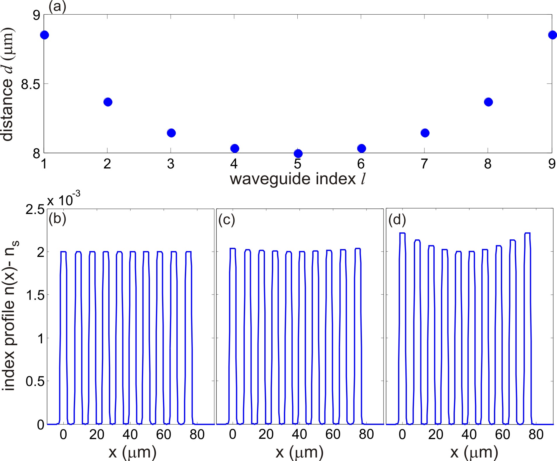
Figure 1: (color online) (a) Distribution of waveguide distance ($d_{l}$ is the distance between waveguides $(l-1)$ and $l$, $l=1,2,...,9$) in a waveguide array composed by $N+1=10$ waveguides that realizes the distribution of the coupling constants defined by Eq.(4) for $J=0.0781\;{\rm mm}^{-1}$. The panels (b-d) show the refractive index profile $n(x)-n_{s}$ of the waveguide arrays that realize the Bose-Hubbard Hamiltonian for increasing values of the interaction strength $U$: in (b) $U=0$, in (c) $U=0.0174\;{\rm mm}^{-1}$, whereas in (d) $U=0.1043\;{\rm mm}^{-1}$.

where $\lambdabar=\lambda/(2\pi)$ is the reduced wavelength of photons (for details see, for instance, [29]). In particular, to independently engineer the coupling constants $\kappa_{l}$ and propagation constant shifts $V_{l}$ of the waveguides, one can assume a chain of waveguides with equal normalized refractive index profile $g(x)$, but with different index contrasts $\Delta n_{l}$ ($l=0,1,2,...,N$) and spacing $d_{l}=x_{l}-x_{l-1}$ ($l=1,2,...,N$), i.e.

$$n(x)-n_{s}=-\sum_{l=0}^{N}\Delta n_{l}g(x-x_{l}).$$ (6)

As discussed in the example below, to realize the Bose-Hubbard lattice (3) the values of $d_{l}$ and $\Delta n_{l}$ slightly vary around some mean values $d_{r}$ and $\Delta n$ that define a uniform array. The waveguide separation $d_{l}$ mainly determines the value of the coupling rate $\kappa_{l-1}$, with a characteristic exponential dependence of $\kappa_{l-1}$ from $d_{l}$, whereas the index change $\Delta n_{l}$ mainly defines the propagation constant mismatch $V_{l}$. It is worth noticing that, in the absence of particle interaction, i.e. for $U=0$, the lattice model (3) associated to the Bose-Hubbard Hamiltonian was previously introduced in the photonic context to realize exact spatial beam self-imaging in finite waveguide arrays [27] and shown to belong to a rather general class of exactly-solvable self-imaging tight-binding lattices with equally-spaced energy levels [28]. A nonvanishing value of the interaction strength $U$ breaks the periodic self-imaging property of the array and enables to visualize with light waves the rich dynamical features of the two-site Bose-Hubbard Hamiltonian directly in the Fock space (see, for instance, [2, 3, 4, 5, 6, 7, 8, 9, 14, 15, 16, 17] and references therein). Here two important dynamical features will be considered for the sake of example, namely (i) the transition from Josephson-like oscillations to self-trapping as the interaction $U$ is increased [2, 3, 9], and (ii) the transition from single-atom to correlated pair tunneling of two bosons in a double well potential [8, 30].

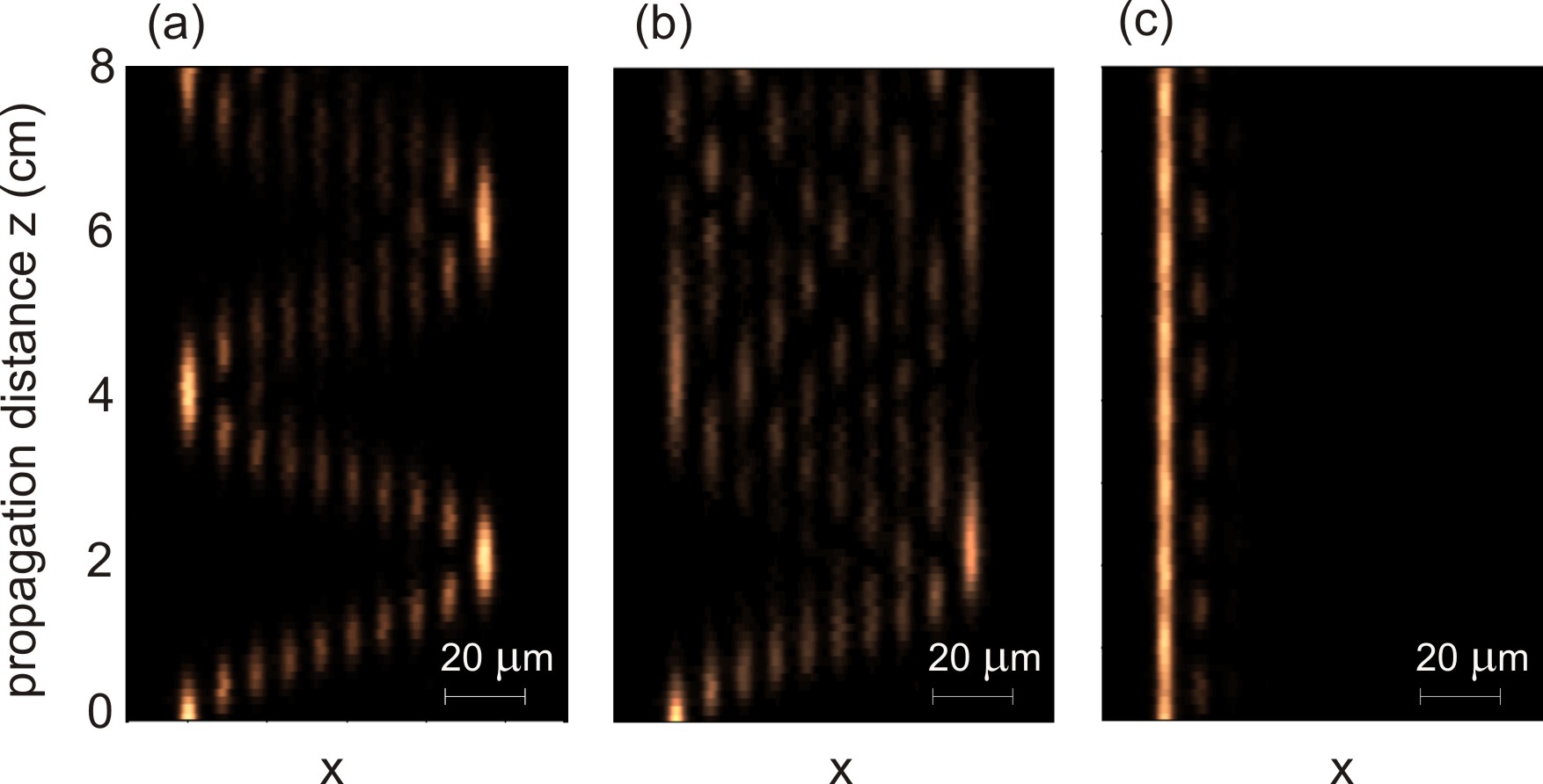
Figure 2: (color online) Light intensity evolution (snapshot of $\phi(x,z)|^{2}$) in the three waveguide arrays of Figs.1(b-d) corresponding to excitation of the left boundary waveguide, as obtained by numerical simulations of the paraxial wave equation (5). The images in (a), (b) and (c) correspond to the Bose-Hubbard Hamiltonian for increasing values of the interaction strength $U$ (from left to right).

To visualize the first effect, we specifically design three arrays comprising $N+1=10$ waveguides, which mimic the evolution of $N=9$ atoms in a double well, for three increasing values of the interaction $U$. The arrays were designed to operate at $\lambda=633$ nm in a transparent glass with a bulk refractive index $n_{s}=1.45$ and with a normalized waveguide channel profile $g(x)=\{{\rm erf}[(x+w)/D_{x}]-{\rm erf}[(x-w)/D_{x}]\}/[2{\rm erf}(w/D_{x})]$ with channel width $2w=4\;\mu$m and diffusion length $D_{x}=0.3\;\mu{\rm m}^{-1}$. The distances between waveguides $d_{l}$ were designed to realize the coupling rates $\kappa_{l}$ given Eq.(4) with $J=0.0781\;{\rm mm}^{-1}$. To determine the distribution of distances $d_{l}$, a reference value $\Delta n=2\times 10^{-3}$ of refractive index contrast was assumed, and correspondingly the coupling rate $\kappa$ between two adjacent waveguides versus distance $d$ was computed, yielding to a good approximation the exponential dependence $\kappa(d)=\kappa_{0}\exp[-\gamma(d-d_{r})]$ for distances not too far from the reference distance $d_{r}=8\;\mu$m, where $\kappa_{0}\simeq 0.3907\;{\rm mm}^{-1}$ and $\gamma\simeq 0.6\;\mu{\rm m}^{-1}$. The resulting distance distribution, depicted in Fig.1(a), shows that the waveguide distances slightly vary around the reference value $d_{r}$ indeed. By modulating the index contrasts $\Delta n_{l}$ of the waveguides around the reference value $\Delta n$, three different arrays were then designed to realize the three different interaction regimes $U=0$, $U=0.0174\;{\rm mm}^{-1}$, and $U=0.1043\;{\rm mm}^{-1}$, as shown in Figs.1(b-d) [31]. Such arrays could be fabricated in fused silica by the recently developed femtosecond laser writing technique [20], in which the different refractive index contrasts are obtained by varying the speed of the writing laser beam. Figures 2 show the evolution of light intensity $|\phi(x,z)|^{2}$ along the three arrays, as obtained by numerical simulations of Eq.(5) using a standard pseudospectral split-step method, when the left boundary waveguide is excited at the input plane. Such an excitation corresponds to the initial conditions $c_{l}(0)=\delta_{l,0}$, i.e. to the entire $N$ bosons in the right well at the initial time. Note that in case $U=0$ [Fig.2(a)] periodic self-imaging of the light pattern is observed because of the equispacing of the energy levels of the Bose-Hubbard Hamiltonian. Such periodic oscillations of the light intensity pattern, previously predicted in Ref.[27] and referred to as harmonic oscillations, are thus the optical analogue of the bosonic Josephson oscillations in the non-interacting regime [2]. A quantitative measure of the Josephson oscillations, generally used in the atom optics context, is provided by the normalized population imbalance $P(z)$, which is defined as the normalized difference between the average numbers of atoms in the two wells, i.e. $P(z)=\sum_{l=0}^{N}[(N-2l)/N]|c_{l}|^{2}$. Note that in an optical experiment $P(z)$ can be retrieved from a measurement of the beam center of mass position $\langle x(z)\rangle=\int dxx|\phi(x,z)|^{2}/\int dx|\phi(x,z)|^{2}$ using the simple relation $P(z)\simeq 1-2\langle x(z)\rangle/(Nd_{r})$. For the $U=0$ case, the evolution of $P(z)$ along the array is depicted in Fig.3(a) and compared to the exact curve obtained from the tight-binding lattice model (3). Note that $P(z)$ oscillates between -1 and 1 with spatial period $z_{R}=\pi/J\simeq 4$ cm, which is precisely the period of Josephson oscillations of the bosonic junction in the absence of interaction. As the interaction strength is increased, the self-imaging property of the array is clearly broken [see Figs. 2(b) and (c)], with a clear transition to damped Josephson oscillations [Fig.3(b)] and to the self-trapping regime [Fig.3(c)]. It should be noted that the mean-field limit of the two-site Bose-Hubbard model in the large $N$ limit, which is described by two nonlinear coupled mode equations [2, 9], could be realized in an optical setting by a simple nonlinear optical directional coupler [32], and self-trapping phenomena in such nonlinear couplers have been previously investigated. However, our waveguide lattice system provides an exact realization of the Bose-Hubbard model even for a low number of particles (as in the example previously discussed) where the mean field approximation fails.

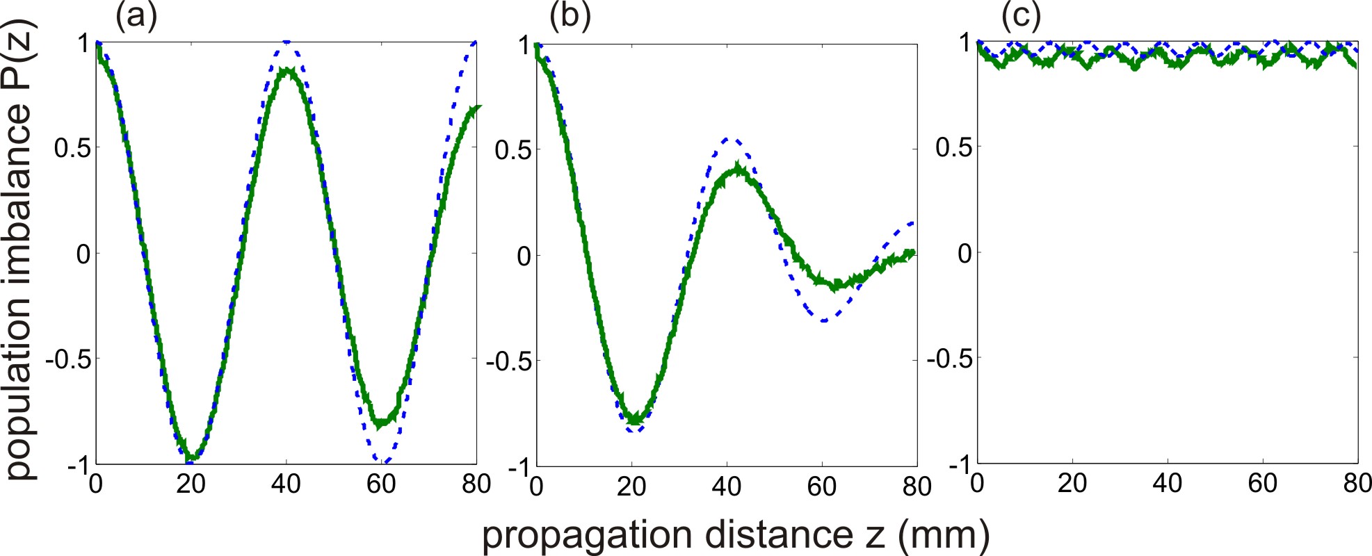
Figure 3: (color online) Behavior of the numerically-computed population imbalance $P(z)$ for the three waveguide arrays of Fig.2 (solid curves), and corresponding behavior predicted by the tight-binding Bose-Hubbard Hamiltonian (3). From (a) to (c), the interaction strength takes the values $U=0$, $U=0.0174\;{\rm mm}^{-1}$, and $U=0.1043\;{\rm mm}^{-1}$.

As a second example, we discuss the phenomenon of correlated pair tunneling of two bosons in a double well potential induced by interaction, which was investigated theoretically and experimentally in previous works (see, for instance, [8, 30]). Even if the two-mode Bose-Hubbard model is capable of describing the dynamics of such a system solely for weak interactions and far from the fragmentation regime [30], it well explains the transition from Rabi oscillations of single particles to correlated pair tunneling in the presence of a weak interaction. Such a kind of correlated dynamics of a pair of interacting atoms was experimentally observed in Ref.[8] by recording both the atom position and phase coherence over time, and was explained on the basis of the simplified Bose-Hubbard Hamiltonian (2). In the $N=2$ particle case, the coupled-mode equations (3) reduce to the following ones

$$i\frac{dc_{0}}{dt} = -\sqrt{2}Jc_{1}+Uc_{0}$$

$$i\frac{dc_{1}}{dt} = -\sqrt{2}J(c_{0}+c_{2})$$ (7)

$$i\frac{dc_{2}}{dt} = -\sqrt{2}Jc_{1}+Uc_{2}.$$

The tunneling dynamics can be analyzed by the introduction of the percentage of bosons in the right well, $p_{R}(t)=|c_{0}(t)|^{2}+(1/2)|c_{1}(t)|^{2}$, and the pair (or same-site) boson probability $p_{2}(t)=|c_{0}(t)|^{2}+|c_{2}(t)|^{2}$ [30], i.e. the probability to find the two bosons in the same well (either the left or the right well). The evolution of the particle occupation probabilities $|c_{l}(t)|^{2}$ can be readily obtained by solving Eq.(7) with the initial condition $c_{0}(0)=1$ and $c_{1}(0)=c_{2}(0)=0$. One obtains

$$|c_{1}(t)|^{2} = \frac{2J^{2}}{M^{2}}\sin^{2}(Mt)$$

$$|c_{2}(t)|^{2} = \frac{1}{4}\left[1+\cos^{2}(Mt)-2\cos\left(\frac{Ut}{2}\right)\cos(Mt)\right.$$ (8)

$$- \left.\frac{U}{M}\sin\left(\frac{Ut}{2}\right)\sin(Mt)+\frac{U^{2}}{4M^{2}}\sin^{2}(Mt)\right]$$

$$|c_{0}(t)|^{2} = 1-|c_{1}(t)|^{2}-|c_{2}(t)|^{2}$$

where we have set $M=\sqrt{4J^{2}+U^{2}/4}$. Correspondingly, the behavior of $p_{R}(t)$ and $p_{2}(t)$ reads

$$p_{R}(t) = 1-\frac{J^{2}}{M^{2}}\sin^{2}(Mt)-\frac{1}{4}\left[1+\cos^{2}(Mt)-2\cos\left(\frac{Ut}{2}\right)\cos(Mt)\right.$$ (9)

$$- \left.\frac{U}{M}\sin\left(\frac{Ut}{2}\right)\sin(Mt)+\frac{U^{2}}{4M^{2}}\sin^{2}(Mt)\right]$$

$$p_{2}(t) = 1-\frac{2J^{2}}{M^{2}}\sin^{2}(Mt)$$ (10)

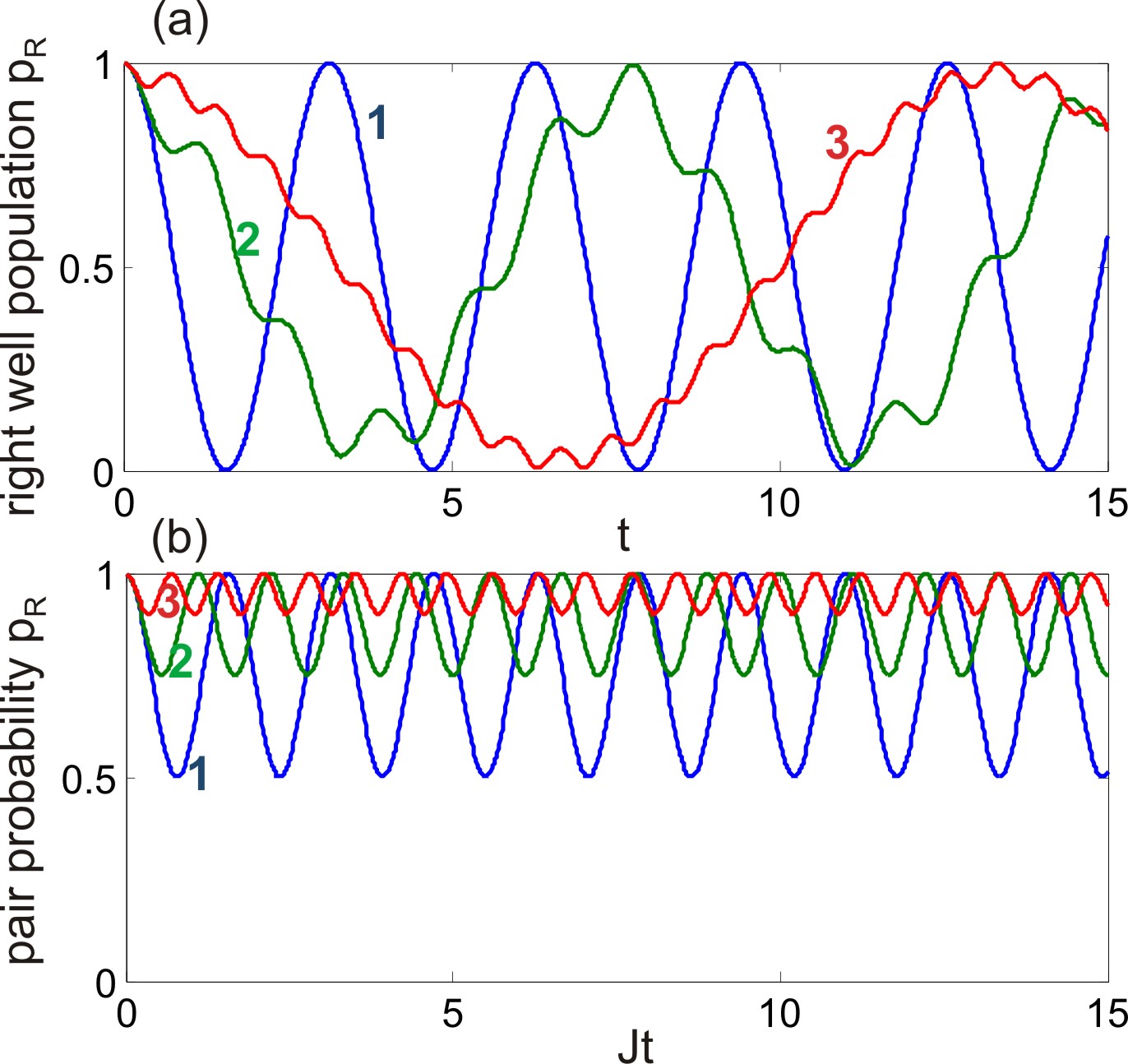
Figure 4: (color online) Behavior of (a) the percentage of bosons in the right well $p_{R}(t)$, and (b) of the pair (same-site) boson probability $p_{2}(t)$ in the Bose-Hubbard model with two atoms for for increasing values of the intercation strength $U$, normalized to the hopping rate $J$. Curve 1: $U/J=0$; curve 2: $U/J=4$; curve 3: $U/J=8$.

A typical behavior of both $p_{R}(t)$ and $p_{2}(t)$ for increasing values of the ratio $U/J$ is shown in Figs.4(a) and (b), respectively. Note that, for the non-interacting case ($U=0$, curve 1 in Fig.4) the atoms simply Rabi oscillate back and forth between both wells, and they tunnel independently. As a correlation is introduced, the tunneling becomes a two-mode process and the tunneling period increases [curves 2 and 3 in Fig.4(a)]. More interestingly, from the behavior of $p_{2}(t)$ one can see that as the interaction is increased both atoms remain essentially in the same well in the course of tunneling, i.e they tunnel as pairs and the amplitude $c_{1}(t)$ gets negligible [30]. In our optical setting, such a dynamical behavior simply describes light tunneling among three coupled waveguides, with the same coupling rate but with the propagation constant of the central waveguide detuned from that of the outer waveguides [see Eq.(7)], the detuning being proportional to the interaction strength $U$ in the quantum mechanical analogue. Such an optical structure was recently proposed and realized for the observation of an optical analogue of two-photon Rabi oscillations in Ref.[33]. Indeed, the large interaction regime $|U/J|\gg 1$ of the Bose-Hubbard model, corresponding to $|c_{1}(t)|\ll 1$ and to pair tunneling (also referred to as second-order tunneling [8]), leads to Rabi oscillations of light power between the outer waveguides of the triplet system, with small excitation of the central waveguide.

In conclusion, a photonic realization of the two-site Bose-Hubbard Hamiltonian in engineered waveguide lattices has been proposed. Such an optical setting enables to visualize in the Fock space the main dynamical aspects of interacting bosons. In particular, waveguide lattices have been designed to visualize the transition from Josephson-like oscillations to self-trapping, as well as the transition from single-atom to correlated pair tunneling in a simple two-boson system. It is envisaged that the idea proposed in this work to use engineered waveguide lattices to simulate in a purely classical setting the quantum physics of interacting particles should motivate further theoretical and experimental studies. For example, longitudinal modulation of the refractive index in the lattice or the introduction of balanced loss and gain in the waveguides might be used to mimic the recently proposed kicked Bose-Hubbard [12] and non-Hermitian PT-symmetric Bose-Hubbard models [34, 35].

This work was supported by the Italian MIUR (Grant No. PRIN-20082YCAAK).

References

References

- [1] Fisher M P A, Weichman P B, Grinstein G and Fisher D S 1989 Phys. Rev. B 40 546
- [2] Smerzi A, Fantoni S, Giovanazzi S and Shenoy S R 1997 Phys. Rev. Lett. 79 4950
- [3] Milburn G J, Corney J, Wright E M and Walls D F 1997 Phys. Rev. A 55 4318
- [4] Leggett A J 2001 Rev. Mod. Phys. 73 307
- [5] Albiez M, Gati R, Fölling J, Hunsmann S, Cristiani M and Oberthaler M K 2005 Phys. Rev. Lett. 95 010402
- [6] Schumm T, Hofferberth S, Andersson L M, Wildermuth S, Groth S, Bar-Joseph I, Schmiedmayer J and Krüger P 2005 Nat. Phys. 1 57
- [7] Gati R, Hemmerling B, Fölling J, Albiez N and Oberthaler M K 2006 Phys. Rev. Lett. 96 130404
- [8] Fölling S, Trotzky S, Cheinet P, Feld M, Saers R, Widera A, Müller T and Bloch I 2007 Nature (London) 448 1029
- [9] Gati R and Oberthaler M K 2007 J. Phys. B. 40 R61
- [10] Mueller E J, Ho T-L, Ueda M and Baym G 2006 Phys. Rev. A 74 033612
- [11] Zhou Y, Zhai H, R. Lü, Xu Zh and Chang L 2003 Phys. Rev. A 67, 043606
- [12] Strzys M P, Graefe E M and Korsch H J 2008 New J. Phys. 10 013024
- [13] Gong J, Morales-Molina L, and Hänggi P 2009 Phys. Rev. Lett. 103 133002
- [14] Mahmud K W, Perry H and Reinhardt W P 2005 Phys. Rev. A 71 023615
- [15] E.M. Graefe and H. J. Korsch, Phys.Rev.A 76, 032116 (2007).
- [16] Shchesnovich V S and Trippenbach M 2008 Phys. Rev. A 78 023611
- [17] Trimborn F, Witthaut D and Korsch H J 2009 Phys. Rev. A 79 013608
- [18] Christodoulides D N, Lederer F and Silberberg Y 2003 em Nature (London) 424 817
- [19] Longhi S 2009 Laser and Photon. Rev. 3 243
- [20] Szameit A and Nolte S 2010 J. Phys. B 43 163001
- [21] Trompeter H, Pertsch T, Lederer F, Michaelis D, Streppel U, Bräuer A and Peschel U 2006 Phys. Rev. Lett. 96 023901
- [22] Longhi S, Marangoni M, Lobino M, Ramponi R, Laporta P, Cianci E and Foglietti V 2006 Phys. Rev. Lett. 96 243901
- [23] Szameit A, Garanovich I L, Heinrich M, Sukhorukov A A, Dreisow F, Pertsch T, Nolte S, Tünnermann A and Kivshar Y S 2009 Nat. Phys. 5 271
- [24] Schwartz T, Bartal G, Fishman S and Segev M 2007 Nature (London) 446 52
- [25] Lahini Y, Avidan A, Pozzi F, Sorel M, Morandotti R, Christodoulides D N and Silberberg Y 2008 Phys. Rev. Lett. 100 013906
- [26] Perez-Leija A, Moya-Cessa H, Szameit A Christodoulides D N 2010 Opt. Lett. 35 2409
- [27] Gordon R 2004 Opt. Lett. 29 2752
- [28] Longhi S 2010 Phys. Rev. B 82 041106
- [29] Longhi S 2006 Phys. Lett. A 359 166
- [30] Zöllner S, Meyer H D and Schmelcher P 2008 Phys. Rev. Lett. 100 040401
- [31] A numerical computation of the propagation constant of the channel waveguide indicates that a propagation constant shift is approximately obtained by assuming a refractive index constrast , where is the reference value of the index constrast and is a numerical factor of order one ( for the chosen error function waveguide profile).
- [32] Jensen S M 1982 IEEE J. Quantum Electron. 18 1580
- [33] Ornigotti M, Della Valle G, Toney Fernandez T, Coppa A, Foglietti V, Laporta P and Longhi S 2008 J. Phys. B 41 085402
- [34] Graefe E M, Korsch H J and Niederle A E 2008 Phys. Rev. Lett. 101 150408
- [35] Graefe E M, Guenther U, Korsch H J and Niederle A E 2008 J. Phys. A 41 255206