On the Stability of a Chain of Phase Oscillators

Abstract

We study a chain of $N+1$ phase oscillators with asymmetric but uniform coupling. This type of chain possesses $2^{N}$ ways to synchronize in so-called travelling wave states, i.e. states where the phases of the single oscillators are in relative equilibrium. We show that the number of unstable dimensions of a travelling wave equals the number of oscillators with relative phase close to $\pi$. This implies that only the relative equilibrium corresponding to approximate in-phase synchronization is locally stable. Despite the presence of a Lyapunov-type functional periodic or chaotic phase slipping occurs. For chains of length $3$ and $4$ we locate the region in parameter space where rotations (corresponding to phase slipping) are present.

I Introduction

Investigations of synchronized behavior of coupled nonlinear oscillators permeate physics strogatz1988csl ; kuramoto1985cdo , chemistry bareli1985scc ; crowley1989ets , biology kawato1980tcn and engineering ijspeert2001ccp . Dating back to Huyghens, this problem has been explored both mathematically and experimentally. The groundbreaking work of Kuramoto kuramoto2003cow led to the realization that synchronization is a ubiquitous behavior in nature and can be explained by simple models for interaction between components of a system (see for example the excellent review of Strogatz strogatz2000kce ).

Cohen et al. cohen1982ncs studied a chain of Kuramoto oscillators to explain the so-called fictive swimming observed in the Central Pattern Generator (CPG) of the primitive vertebrate lamprey. Their purpose was to explain the uniform phase lag along the segmental oscillators. Later, Kopell and Ermentrout kopell1988coa proposed a more realistic model for fictive swimming and Williams et al. williams1990fcn contrasted this model with experimental observations. Studies of the CPG led to bio-inspired applications in robotics, for example, the autonomous mobile robotic worm of Conradt and Varshavskaya conradt2003dcp and a turtle-like underwater vehicle by Seo et al. seo2008cbc .

Cohen et al. cohen1982ncs observed that in a chain of oscillators the oscillators at the end points play as special role: adapting the natural frequency of the end points controls the phase shift between neighboring oscillators throughout the entire chain in the phase-locked equilibrium. (All equilibria of the one-dimensional homogeneous Kuramoto model with periodic boundary conditions were found in mehta2011stationary .)

In this paper we vary this detuning $\delta$ of the end points and the coupling strength (more precisely the ratio $k$ between coupling strength down the chain and up the chain) to study transitions between phase locked solutions and phase slipping. If one introduces the phase differences between the oscillators as the new dependent variables then the phase-locked solutions are equilibria, and for a chain of length $N+1$ there exist $2^{N}$ of these equilibria. A transition from one phase locked solution to another then corresponds to a motion along a heteroclinic connection between the corresponding saddles in the phase space. The $2^{N}$ equilibria can be classified by an index quantity $\nu_{\pi}$ which counts how many of the phase differences are equal to $\pi-\delta$. This index turns out to be identical to the number $\nu_{u}$ of unstable dimensions of the saddle (provided $k>-1$) such that connections between equilibria of decreasing index $\nu_{\pi}$ are generic. Solutions with continuously slipping phases between oscillators show up as rotating waves in the phase space. Periodic phase slipping and its bifurcations can be computed directly if one assumes, for example, pure phase coupling (coupling of the type $K\sin(\theta_{j}-\theta_{j-1})$ for neighboring oscillators $\theta_{j}$ and $\theta_{j+1}$). One of the co-dimension $1$ boundaries of rotating waves are non-generic connections between equilibria of identical index $\nu_{\pi}$. We present numerical evidence of this for the cases of $N=2$ and $N=3$ (that is, the case of $3$ and $4$ oscillators, respectively). A noticeable difference between these cases is that the basin of attraction for rotating waves appears to be a slightly smaller fraction of the phase space for larger $N$, and the parameter region in the $(k,\delta)$-plane permitting rotations (that is, continuous phase slipping) is smaller for the larger $N$. We conjecture that making an oscillator chain longer does not make its propensity for phase slipping larger even if the coupling strength between neighboring oscillators is not increased.

II Model Description

We consider a chain of $N+1$ phase oscillators with nearest neighbor coupling as shown in Fig. 1.

Figure 1: Schematic representation of chain coupled oscillators

This model, first proposed by Cohen et al. cohen1982ncs to explain the ’fictive swimming’ observed in Lamprey spinal cord, is given by

$$\begin{split}\frac{d}{dt}\theta_{0}&=\omega_{0}+K_{u}\Gamma(\theta_{1}-\theta_{0})\mbox{,}\\ \frac{d}{dt}\theta_{j}&=\omega_{j}+K_{d}\Gamma(\theta_{j-1}-\theta_{j})+K_{u}\Gamma(\theta_{j+1}-\theta_{j})\\ &\qquad\mbox{\ for $j=1,2,\ldots,N-1$,}\\ \frac{d}{dt}\theta_{N}&=\omega_{N}+K_{d}\Gamma(\theta_{N-1}-\theta_{N})\mbox{,}\end{split}$$ (1)

where $\theta_{j}$ and $\omega_{j}\neq 0$ are the phase and natural frequency of the $j$-th oscillator, respectively. The coupling gains are denoted by $K_{u}$ and $K_{d}$. The prototypical example for the coupling function is $\Gamma(x)=\sin x$. This choice of the coupling function has the following essential features:

1. $\Gamma$ is $2\pi$-periodic, $\left|\Gamma(x)\right|\leq 1$,

2. $\Gamma(x)$ has odd symmetry about $x=0$ (that is, $\Gamma(x)=-\Gamma(-x)$) and even symmetry about $x=\pi/2$ (that is, $\Gamma(\pi/2-x)=\Gamma(\pi/2+x)$),

3. $\Gamma^{\prime}(x)>0$ for $x\in[0,\pi/2]$.

III Phase Locking and Traveling Waves

Since the frequencies $\omega_{j}$ are non-zero, system (1) does not in general have fixed points. If all oscillators are identical (that is, $\omega_{0}=\ldots=\omega_{N}$) Equation (1) admits a fully synchronised state $\theta_{0}=\ldots=\theta_{n}$. Here we focus on the so-called phase locked solutions, that is, solutions of the form $\theta_{i}-\theta_{j}=\operatorname{const}$. Of particular importance are phase locked solutions where the phase differences on the chain are identical, called uniform traveling waves.

To analyze phase locked solutions we introduce the phase differences

$$x_{j}=\theta_{j-1}-\theta_{j}\mbox{\quad($j=1\ldots N$)},$$ (2)

as new variables, as well as the rescaled frequency differences $\Omega_{j}$, the coupling ratio $k$ and the rescaled time $t_{\mathrm{new}}$:

$$\Omega_{j}=\frac{\omega_{j-1}-\omega_{j}}{K_{u}}\mbox{\quad($j=1\ldots N$),}k=\frac{K_{d}}{K_{u}}\mbox{,}t_{\mathrm{new}}=K_{u}t\mbox{.}$$

System (1) leads to a system of $N$ equations describing the dynamics of the variables $x_{j}$ wrt the new time $t_{\mathrm{new}}$

$$\begin{split}\dot{x}_{1}&=\Omega_{1}-(1+k)\Gamma(x_{1})+\Gamma(x_{2})\mbox{,}\\ \dot{x}_{i}&=\Omega_{i}+k\Gamma(x_{i-1})+\Gamma(x_{i+1})-(1+k)\Gamma(x_{i})\mbox{,}\\ &\mbox{\qquad$i=2,3,\dots,N-1$,}\\ \dot{x}_{N}&=\Omega_{N}+k\Gamma(x_{N-1})-(1+k)\Gamma(x_{N})\mbox{,}\end{split}$$ (3)

where $x_{i}(t)$ is on the unit circle $\mathbb{S}^{1}$. The vector form reads

$$\dot{\mathbf{x}}=\mathbf{\Omega}+C\mathbf{\boldsymbol{\Gamma}}(\mathbf{x})\mbox{,}$$ (4)

where $\mathbf{x}=[x_{1},x_{2},\cdots,x_{N}]^{T}$, $\mathbf{\Omega}=[\Omega_{1},\Omega_{2},\cdots,\Omega_{N}]^{T}$, $\mathbf{\boldsymbol{\Gamma}}(\mathbf{x})=[\Gamma(x_{1}),\ldots,\Gamma(x_{N})]$, and $C$ is an $N\times N$ matrix of the form

$$C=\begin{bmatrix}-(1+k)&1&\cdots&0\\ k&-(1+k)&\ddots&0\\ \vdots&\ddots&-(1+k)&1\\ 0&0&k&-(1+k)\end{bmatrix}.$$ (5)

The fixed points of Equation (4) are given by $\mathbf{\Gamma}(\mathbf{x})=-C^{-1}\mathbf{\mathbf{\Omega}}$ ($C$ is invertible for $k\neq-1$, see Proposition 2) and correspond to the phase locked solutions satisfying $\theta_{i}-\theta_{j}=\operatorname{const}$ of the original system (1).

If all components of $-C^{-1}\mathbf{\mathbf{\Omega}}$ are less than $1$ in absolute value, system (4) has $2^{N}$ equilibria, because of the even symmetry about $\pi/2$ ($\Gamma(\pi/2-x)=\Gamma(\pi/2+x)$, see Section 2) of the coupling function. A uniform traveling wave solution (phase locked solution with identical phase differences, i.e. $\mathbf{x}=[\delta,\cdots,\delta]^{T}$)) exists only if the following conditions on the rescaled frequency differences $\Omega$ are satisfied:

$$\Omega_{1\,\phantom{-1}} =k\Gamma(\delta)\mbox{,}$$ (6)

$$\Omega_{i\ \phantom{-1}} =0\mbox{,} i =2,\dots,N-1\mbox{,}$$

$$\Omega_{N} =\Gamma(\delta)\mbox{.}$$

This means that the frequencies $\omega_{j}$ of the original system (1) must be of the form

$$\omega_{0} =\omega+K_{d}\Gamma(\delta)\mbox{,}$$ (7)

$$\omega_{j} =\omega\mbox{,} j =1,\dots,N-1\mbox{,}$$

$$\omega_{N} =\omega-K_{u}\Gamma(\delta)\mbox{,}$$

where $\omega\in\mathbb{R}$. In other words, all oscillators must have identical natural frequencies except for the two oscillators at the boundary. The “detunings” (difference from the uniform frequency $\omega$) of the first and last oscillators are related to one another via the coupling strengths $K_{u}$ and $K_{d}$.

The two primary parameters affecting the dynamics are the coupling strength ratio $k$ and $\delta$. Without loss of generality we can restrict our considerations to the parameter set

• $\delta\in[0,\pi/2]$: only $\Gamma(\delta)$ enters the equation and for negative $\delta$ we can apply the transformation $x\mapsto-x$ since $\Gamma$ is odd.

• $k\geq-1$: for $k<-1$ we can apply the transformation $[x_{1},\ldots,x_{N}]_{\mathrm{new}}=[x_{N},\ldots,x_{1}]_{\mathrm{old}}$, $t_{\mathrm{new}}=k_{\mathrm{old}}t$, and $k_{\mathrm{new}}=-1/k_{\mathrm{old}}$ such that $k_{\mathrm{new}}>0$. Note that this transformation involves reversal of time direction (since $k_{\mathrm{old}}$ is negative) so statements on stability will have to be replaced by the corresponding statements on instability and vica versa.

We observe that the coupling strength does not enter Equation (3), which determines the dynamics, at all. Only the ratio between down-chain and up-chain coupling strength matters. The absolute value of the coupling strength then determines the time scale with respect to the the original time (Equation (3) is with respect to a rescaled time $K_{u}t$).

IV Stability of Traveling Waves

Naturally, we are interested in characterizing the local stability of traveling waves, that is, of equilibria of (4). We note that even though the uniform traveling waves can occur only in a slightly degenerate parameter setting, these waves are robust in the sense that slightly non-uniform traveling waves will exist for slight perturbations of these parameters values. For example, non-uniform traveling waves exist for a linear gradient frequency distribution ($\Omega=\operatorname{const}.$). Cohen et al. cohen1982ncs derived a necessary condition for the existence of the phase-locked solutions. Ermentrout and Kopell ermentrout1984fpc showed the existence of frequency plateaus when this necessary condition is violated.

The linearization of (4) about an equilibrium $x_{*}$ is $J=C\mathbf{\boldsymbol{\Gamma\mathrm{{}^{\prime}}}}(x_{*})$ where $C$ is the coupling matrix given in (5), and

$$\boldsymbol{\Gamma}^{\prime}(x_{*})=\rho\cdot\operatorname{diag}(\sigma_{1},\dotsc,\sigma_{n}),$$ (8)

is a diagonal matrix with $\rho=\Gamma^{\prime}(\delta)>0$ (since $\delta\in[0,\pi/2]$) and $\sigma_{i}=\pm 1$, depending on whether the $i$th component of $x_{*}$ is equal to $\delta$ or $\pi-\delta$. Even though the eigenvalues of the matrix $C$ are known, i.e.

$$\lambda_{j}=-(1+k)+2\sqrt{k}\cos\frac{j\pi}{N+1},\mbox{}j=1,\dots,N,$$ (9)

the eigenvalues of the product $C\mathbf{\boldsymbol{\Gamma\mathrm{{}^{\prime}}}}(x_{\ast})$ are not known analytically. Therefore, the goal of this Section is to establish a simple connection between the number of stable and unstable directions of an equilibrium $x_{\ast}$ (and thus its stability) of (4) and the number of components of $x_{\ast}$ equal to $\delta$ and $\pi-\delta$. To establish the result, we associate the four indices with each equilibrium $x_{\ast}$

$$\begin{split}\nu_{0}(x_{\ast})&=\ \mbox{number of components of $x_{*}$ equal to $\delta$,}\\ \nu_{\pi}(x_{\ast})&=\ \mbox{number of components of $x_{*}$ equal to $\pi-\delta$,}\\ \nu_{u}(x_{\ast})&=\ \mbox{dimension of unstable manifold of $x_{*}$,}\\ \nu_{s}(x_{\ast})&=\ \mbox{dimension of stable manifold of $x_{*}$.}\end{split}$$ (10)

The relation between these indices is given by the following

Theorem 1 (Dimension of invariant subspaces).

Let $x_{*}$ be an equilibrium of (4). If $k>-1$ then

$$\nu_{0}(x_{*})=\nu_{s}(x_{*})\mbox{\ and\ }\nu_{\pi}(x_{*})=\nu_{u}(x_{*})\mbox{.}$$ (11)

Proof

Relation (11) is proven indirectly via the Lyapunov-type functional

$$E(x)=\sum_{i=1}^{N}\left[\int_{0}^{x_{i}}\Gamma(y)\,y-\Gamma(\delta)\,x_{i}\right]\mbox{.}$$ (12)

We observe that the time derivative of $E$ along trajectories of (4) is

$$\begin{split}\dot{E}=&\sum_{i=1}^{N}\left[\Gamma(x_{i})-\Gamma(\delta)\right]\dot{x}_{i}\\ =&-\frac{k+1}{2}\left(\left(\Gamma(x_{1})-\Gamma(\delta)\right)^{2}+\left(\Gamma(x_{N})-\Gamma(\delta)\right)^{2}+\phantom{\sum_{i}^{N}}\right.\\ &\left.+\sum_{i=1}^{N-1}\left(\Gamma(x_{i})-\Gamma(x_{i+1})\right)^{2}\right).\end{split}$$ (13)

If $k=-1$ then $E(x(t))$ is constant along trajectories, however it is strictly decreasing for $k>-1$ provided $x(t)$ is not an equilibrium of (4) (i.e. whenever at least one of the phase differences $x_{i}$ does not satisfy $\Gamma(x_{i})=\Gamma(\delta)$). With this functional $E$ and a bound on its rate of decrease (13) we establish in Appendix A that the linearization $J=C\mathbf{\boldsymbol{\Gamma\mathrm{{}^{\prime}}}}(x_{\ast})$ is hyperbolic for $k>-1$. This implies that eigenvalues of $J$ cannot cross the imaginary axis when $k$ is varied. Thus, for all $k>-1$ the indices $\nu_{u}(x_{\ast})$ and $\nu_{s}(x_{\ast})$ are the same as for $k=0$. Since for $k=0$ the Jacobian $J$ is an upper diagonal matrix with its eigenvalues on its diagonal, the number of negative diagonal entries of $J$ is $\nu_{0}(x_{\ast})$ (the diagonal entry of $C$ is $-1$), and the number of positive diagonal entries of $J$ is $\nu_{\pi}(x_{\ast})$. $\square$

We observe that for $\delta=0$ the functional $E(x)$ is bounded, leading for $k\neq 1$ to the result that full synchronization (the equilibrium $(0,\ldots,0)$ for $\delta=0$) is globally stable in the same way as the classical results hoppensteadt1997weakly .

V Rotating waves and saddle connections

Despite the existence of a Lyapunov functional the dynamics of (4) is not necessarily trivial because the phase space is an $N$-dimensional torus. Generically we can expect that the unstable manifold of an equilibrium $x$ and the stable manifold of an equilibrium $y$ intersect, giving rise to heteroclinic saddle connections, if $\nu_{\pi}(x)+\nu_{0}(y)>N$. This implies that for any equilibrium $x$ heteroclinic connections to all equilibria $y$ satisfying $\nu_{\pi}(y)<\nu_{\pi}(x)$ are generic.

Saddle connections between equilibria of the same type, that is $\nu_{\pi}(x)=\nu_{\pi}(y)$, are of co-dimension $1$ and can be achieved by tuning the parameters $\delta$ and $k$. These non-generic saddle connections also form co-dimension $1$ boundaries of periodic orbits of rotating wave type.

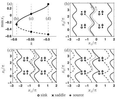
Figure 2: Co-dimension $1$ homoclinic connections and rotating waves for $N=2$, $\Gamma(x)=\sin x$ and $\delta=1$. (a): bifurcation diagram for rotating wave solutions (computed with (r)AUTO DCFKSW98 ; S07 ), (b)–(d): phase portraits showing equilibria homoclinic connections and rotating waves for parameter values of $k$ indicated in panel (a). The direction of the flow is always upward.

Figure 2(a) shows for $N=2$ that periodic orbits (of rotating wave type) are possible for a range of parameters $k$ and $\delta=1$ despite the existence of a Lyapunov functional $E$. In the parameter space the existence of periodic orbits is bounded by two co-dimension $1$ bifurcations: a saddle-node of periodic orbits corresponding to the phase portrait in Figure 2(b) at the minimal $k$ supporting periodic orbits and a heteroclinic connection between neighboring saddles (the $x_{2}$-component has increased by $2\pi$ along the heteroclinic connection).

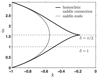
Figure 3: Bifurcation diagram in the $(k,\delta)$-plane for $N=2$ and $\Gamma(x)=\sin x$ (computed with (r)AUTO DCFKSW98 ; S07 ).

If the phase shift by $2\pi$ is ignored then the saddle connection is homoclinic. Figure 3 shows the parameter region in the $(k,\delta)$-plane where periodic orbits of rotating wave type exist. The special points in the plane are at $\delta=\pi/2$ when all four equilibria collapse into a single degenerate equilibrium and at $k=-1$ when the system is a single-degree-of-freedom conservative oscillator for $N=2$. We also note that the diagram is reflection symmetric about the line $\delta=\pi/2$ as expected.

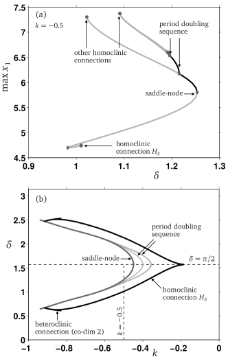
Figure 4: Bifurcation diagrams for $N=3$ and $\Gamma(x)=\sin x$ (computed with (r)AUTO DCFKSW98 ; S07 ). Panel (a): family of periodic orbits for fixed $k=-0.5$ and varying $\delta$ and its codimension-$1$ bifurcations. Panel (b): region with rotating waves in the $(k,\delta)$-plane with its codimension-$1$ bifurcations.

In dimensions $N>2$ the dynamics can become chaotic. Numerical evidence for this is shown in Figure 4 for $N=3$. Panel (a) shows a family of periodic orbits of rotating wave type $(x_{1}(T),x_{2}(T),x_{3}(T))=(x_{1}(0),x_{2}(0)+2\pi,x_{3}(0)+2\pi)$ where $T$ is the period, $\delta$ is varied, and $k=-0.5$ is kept fixed. We observe that this family undergoes a period doubling sequence. Moreover, the lower (predominantly unstable) part of the branch reaches a homoclinic connection to the saddle $x_{s}=(\pi-\delta,\delta,\delta)$ at $H_{s}$. The eigenvalues at this saddle have the form $(\mu_{+},-\mu_{-}\pm i\omega_{-})$ where $\mu_{\pm}>0$ and $\omega_{-}>0$ are real numbers and $\mu_{-}<\mu_{+}<2\mu_{-}$. Shil’nikov’s results imply that there is an infinite number of period doubling cascades of stable periodic orbits close to the homoclinic connection $H_{s}$ (under certain non-degeneracy conditions, see SSTC01 ; K04 ). The precise sequence of period-$n$ branches for a homoclinic to a saddle of this type, and how to calculate them numerically can be found in OKC00 . The other end of the family of periodic orbits is also a homoclinic connection, to the saddle $(\delta,\pi-\delta,\delta)$, which has three real eigenvalues $\mu_{+}>0>-\mu_{-,1}>-\mu_{-,2}$ where $\mu_{+}>\mu_{-,1}$. This implies that there is only a single periodic orbit close to this homoclinic connection (no snaking), and that this periodic orbit is unstable K04 .

In the two-parameter plane (shown in Figure 4(b)) we observe a shape that looks superficially similar to the case $N=2$ except that the range of $\delta$ over which the region of rotating waves extend is smaller. However, as one can see from Figure 4(a) the rotating waves are not stable inside the region bounded by the homoclinic connection $H_{s}$ and the saddle-node. The period doubling sequence (also shown in Figure 4(a)) gives a better estimate for the region of stable periodic rotating waves. The remainder of the region is not filled with chaotic rotations because the chaotic attractor at the end of the primary period doubling cascade collides with heteroclinic saddle connections. Figure 5 shows a periodic motion of period $8$, which is close to the end of the period doubling sequence in parameter space.

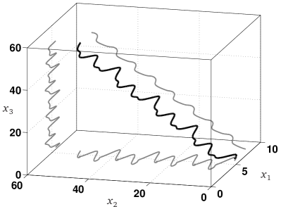
Figure 5: Rotating periodic orbit of period $8$ for $N=3$, $\Gamma(x)=\sin x$, $k=-0.5$, $\delta\approx 1.19$, near the end of the period doubling sequence in parameter space.

Special points in the bifurcation diagram 4(b) are on the symmetry line $\delta=\pi/2$ (where all equilibria collapse to a single degenerate equilibrium) and various degeneracies of the homoclinic connection, for example, the heteroclinic connection $(\pi-\delta,\delta,\delta)\to(2\pi+\delta,\pi-\delta,\delta)\to(\pi-\delta,2\pi+\delta,2\pi+\delta)$ indicated in Figure 4(b) (this degeneracy ends the numerical continuation of the homoclinic).

In the original variables $\theta_{j}$ the rotating waves shown in this Section correspond to a continually drifting phase difference between the oscillators $2$ and $3$ (for $N=2$) while the phase difference between oscillators $1$ and $2$ remains bounded. The homoclinic boundary corresponds to regimes where two neighboring oscillators hover in anti-phase for a long time before a phase slip occurs. For $N=3$ the chaotic regimes near the Shil’nikov saddle correspond to the regime where oscillators $1$ and $2$ are nearly in anti-phase and $2$, $3$ and $4$ are nearly in-phase for a long time before the phase differences between $2$ and $3$, and $3$ and $4$ slip (nearly) simultaneously.

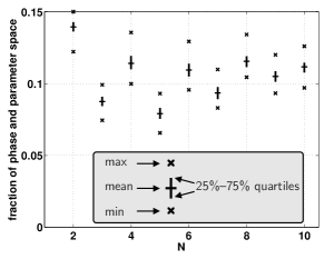
Figure 6: Fraction of phase and parameter space not attracted to synchronization. These are simulation results obtained during $100$ trials where in each trial we chose $5,000$ random initial conditions $x(0)\in\mathbb{S}^{N}$ and random parameters $\delta\in[0,\pi/2]$, $k\in[-1,0]$ for small $N\geq 2$. During each trial simulation we record when a trajectory enters the neighborhood of the stable equilibrium $(\delta,\ldots,\delta)$. We stop the simulation if no new trajectory enters this neighborhood during a time period of $200$. The plot (horizontal line) shows which fraction of the $5,000$ realizations was not yet trapped on average when we stopped the simulation. The vertical lines give the variability between trials ($25\%$ and $75\%$ quartile) and the crosses are the extreme (maximal and minimal) result of the $100$ trials.

As the number of oscillators is increased by $1$, we observe that the parameter region which supports stable periodic rotations shrinks. Put another way, full synchronization becomes more prevalent for $N=3$. The simulation results shown in Figure 6 support this observation. This is in contrast to the common feature that longer chains of oscillators require stronger coupling for synchronization hoppensteadt1997weakly ; Hong2005 in symmetrically coupled chains with random frequencies. The reason behind this apparent difference is that in our setup the only detuned oscillators are at the boundary (indices $0$ and $N$), and that the effect of the boundary diminishes for increasing $N$. We did not observe, however, that the fraction of slipping realizations approaches zero for large $N$.

VI Conclusion

In this paper we studied the dynamical system describing the phase differences of a uniform chain of oscillators. Two important parameters (other than the number of elements in the chain) are the detuning of the end points, $\delta$ and the ratio $k$ of the coupling strengths upward and downward the chain. We have classified the phase locked states by relating the number of phase differences that equal $\pi-\delta$ to the number of unstable directions that this phase locked state has as a saddle in the phase space. We also studied periodic phase slipping (rotating waves) systematically for $N=2$ ($3$ oscillators) and $N=3$ ($4$ oscillators). The most curious difference between the case of $N=2$ and $N=3$ is the shrinking of the parameter region where periodic rotations occur. Simulations suggest that their basin of attraction also shrinks as a fraction of the whole phase space volume. This would suggest that longer chains have more robust phase locking. This effect appears to hold with respect to both aspects of robustness combined: the fraction of initial values (treating parameters also as dynamic variables with trivial dynamics, $\dot{\delta}=0$, $\dot{k}=0$) in the phase space leading to locking is smallest for $N=2$.

Appendix A Proof of hyperbolicity of equilibria

Proposition 2 (Absence of eigenvalues with zero real part).

Let $k>-1$, and let $x_{*}$ be an equilibrium of (4). Then the Jacobian $J=C\boldsymbol{\Gamma}^{\prime}(x_{*})$ of (4) in $x_{*}$ cannot have eigenvalues on the imaginary axis.

Proof

First we note that the matrix $J$ is regular for $k>-1$ (and, thus, cannot have an eigenvalue $0$):

$$\det C = \frac{\left(-1\right)^{N}\left(k^{N+1}-1\right)}{k-1} \neq 0\mbox{,}$$ (14)

$$\det \boldsymbol{\Gamma}^{\prime}(x_{*}) = \Gamma^{\prime}(\delta)^{N}(-1)^{\nu_{\pi}} \neq 0\mbox{.}$$

We show the absence of purely imaginary eigenvalues indirectly. In preparation for this part of the proof we establish a bound on the gradient of Lyapunov functional $E$, given in (12). In an equilibrium $x_{*}$ the gradient of $E$ vanishes and the Hessian $H_{*}$ of $E$ in $x_{*}$ is equal to $\boldsymbol{\Gamma}^{\prime}(x_{*})$:

$$\begin{split}H_{*}=H(x_{*})&=\frac{\partial^{2}}{(\partial x)^{2}}E(x)|_{x=x_{*}}\\ &=\rho\cdot\operatorname{diag}(\sigma_{1},\dotsc,\sigma_{n})=\boldsymbol{\Gamma}^{\prime}(x_{*}).\end{split}$$ (15)

Consequently, the equilibrium $(\delta,\dotsc,\delta)$ is a local minimum of $E$, and $(\pi-\delta,\dotsc,\pi-\delta)$ is a local maximum of $E$. Equilibria which have some components equal to $\delta$ and others equal to $\pi-\delta$ are saddle points of the graph of $E$. As we want to study the local stability of an equilibrium $x_{*}$ we introduce quantities measuring the deviation from $x_{*}$:

$$y=x-x_{*}\mbox{\ and\ }D(y)=E(y+x_{*})-E(x_{*}),$$ (16)

such that $D(0)=0$ and

$$D(y)=y^{T}H_{*}y+O(\|y\|^{3}),$$ (17)

for all $y$ in a neighborhood of $0$. Furthermore, equation (13) estimates $\dot{D}$ from above for $k>-1$:

$$\dot{D}(y)\leq-c_{0}\|y\|^{2}\mbox{,}$$ (18)

where $c_{0}>0$ is a constant independent of $y$.

Assume that $J$ has a purely imaginary eigenvalue, say, $\lambda=i\mu$ where $\mu>0$, and let $u$ be the corresponding eigenvector. We choose the time $T=2\pi/\mu$. Let $\epsilon>0$ be sufficiently small ($\epsilon$ will depend on $T$). After time $T$ the solution of (4) starting from $x(0)=x_{*}+\epsilon u$ (let us call the solution $x(\cdot)$) satisfies $x(T)=x_{*}+\epsilon u+O(\epsilon^{2})$. Consequently,

$$D(x(T)) -D(x(0))=$$

$$=\ [x(T)-x_{*}]^{T}H_{*}[x(T)-x_{*}]+O(\|x(T)-x_{*}\|^{3})$$

$$-\epsilon^{2}u^{T}H_{*}u-O(\epsilon^{3})$$

$$=\ O(\epsilon^{3})\mbox{.}$$ (19)

On the other hand, the trajectory $x(t)$ for $t\in[0,T]$ is a perturbation of order $\epsilon^{2}$ of an ellipse with a minimal radius of order $\epsilon$ around $x_{*}$. This means that we can choose a uniform constant $c_{1}$ of order $1$ such that $c_{1}\epsilon$ is smaller than this minimal radius ($c_{1}$ is uniform in $\epsilon$) and, hence,

$$\|x(t)-x_{*}\|\geq c_{1}\epsilon$$ (20)

for all $t\in[0,T]$. Inequality (18) implies that

$$D(x(T)) -D(x(0))=\int_{0}^{T}\dot{D}(x(t))dt$$

$$\leq-c_{0}\int_{0}^{T}\|x(t)-x_{*}\|^{2}\,dt$$ (due to (18)),

$$\leq-c_{0}Tc_{1}^{2}\epsilon^{2}$$ (due to (20)),

which contradicts (19) because the constants $c_{0}$ and $c_{1}$ are independent of $\epsilon$. $\square$