A Primal-Dual Convergence Analysis of Boosting

Abstract

Boosting combines weak learners into a predictor with low empirical risk. Its dual constructs a high entropy distribution upon which weak learners and training labels are uncorrelated. This manuscript studies this primal-dual relationship under a broad family of losses, including the exponential loss of AdaBoost and the logistic loss, revealing:

• Weak learnability aids the whole loss family: for any $\epsilon>0$, $\mathcal{O}(\ln(1/\epsilon))$ iterations suffice to produce a predictor with empirical risk $\epsilon$-close to the infimum;

• The circumstances granting the existence of an empirical risk minimizer may be characterized in terms of the primal and dual problems, yielding a new proof of the known rate $\mathcal{O}(\ln(1/\epsilon))$;

• Arbitrary instances may be decomposed into the above two, granting rate $\mathcal{O}(1/\epsilon)$, with a matching lower bound provided for the logistic loss.

1 Introduction

Boosting is the task of converting inaccurate weak learners into a single accurate predictor. The existence of any such method was unknown until the breakthrough result of Schapire (1990): under a weak learning assumption, it is possible to combine many carefully chosen weak learners into a majority of majorities with arbitrarily low training error. Soon after, Freund (1995) noted that a single majority is enough, and that $\Theta(\ln(1/\epsilon))$ iterations are both necessary and sufficient to attain accuracy $\epsilon$. Finally, their combined effort produced AdaBoost, which exhibits this optimal convergence rate (under the weak learning assumption), and has an astonishingly simple implementation (Freund and Schapire, 1997).

It was eventually revealed that AdaBoost was minimizing a risk functional, specifically the exponential loss (Breiman, 1999). Aiming to alleviate perceived deficiencies in the algorithm, other loss functions were proposed, foremost amongst these being the logistic loss (Friedman et al., 2000). Given the wide practical success of boosting with the logistic loss, it is perhaps surprising that no convergence rate better than $\mathcal{O}(\exp(1/\epsilon^{2}))$ was known, even under the weak learning assumption (Bickel et al., 2006). The reason for this deficiency is simple: unlike SVM, least squares, and basically any other optimization problem considered in machine learning, there might not exist a choice which attains the minimal risk! This reliance is carried over from convex optimization, where the assumption of attainability is generally made, either directly, or through stronger conditions like compact level sets or strong convexity (Luo and Tseng, 1992). But this limitation seems artificial: a function like $\exp(-x)$ has no minimizer but decays rapidly.

Convergence rate analysis provides a valuable mechanism to compare and improve of minimization algorithms. But there is a deeper significance with boosting: a convergence rate of $\mathcal{O}(\ln(1/\epsilon))$ means that, with a combination of just $\mathcal{O}(\ln(1/\epsilon))$ predictors, one can construct an $\epsilon$-optimal classifier, which is crucial to both the computational efficiency and statistical stability of this predictor.

The main contribution of this manuscript is to provide a tight convergence theory for a large family of losses, including the exponential and logistic losses, which has heretofore resisted analysis. In particular, it is shown that the (disjoint) scenarios of weak learnability (Section 6.1) and attainability (Section 6.2) both exhibit the rate $\mathcal{O}(\ln(1/\epsilon))$. These two scenarios are in a strong sense extremal, and general instances are shown to decompose into them; but their conflicting behavior yields a degraded rate $\mathcal{O}(1/\epsilon)$ (Section 6.3). A matching lower bound for the logistic loss demonstrates this is no artifact.

1.1 Outline

Beyond providing these rates, this manuscript will study the rich ecology within the primal-dual interplay of boosting.

Starting with necessary background, Section 2 provides the standard view of boosting as coordinate descent of an empirical risk. This primal formulation of boosting obscures a key internal mechanism: boosting iteratively constructs distributions where the previously selected weak learner fails. This view is recovered in the dual problem; specifically, Section 3 reveals that the dual feasible set is the collection of distributions where all weak learners have no correlation to the target, and the dual objective is a max entropy rule.

The dual optimum is always attainable; since a standard mechanism in convergence analysis to control the distance to the optimum, why not overcome the unattainability of the primal optimum by working in the dual? It turns out that the classical weak learning rate was a mechanism to control distances in the dual all along; by developing a suitable generalization (Section 4), it is possible to convert the improvement due to a single step of coordinate descent into a relevant distance in the dual (Section 6). Crucially, this holds for general instances, without any assumptions.

The final puzzle piece is to relate these dual distances to the optimality gap. Section 5 lays the foundation, taking a close look at the structure of the optimization problem. The classical scenarios of attainability and weak learnability are identifiable directly from the weak learning class and training sample; moreover, they can be entirely characterized by properties of the primal and dual problems.

Section 5 will also reveal another structure: there is a subset of the training set, the hard core, which is the maximal support of any distribution upon which every weak learner and the training labels are uncorrelated. This set is central—for instance, the dual optimum (regardless of the loss function) places positive weight on exactly the hard core. Weak learnability corresponds to the hard core being empty, and attainability corresponds to it being the whole training set. For those instances where the hard core is a nonempty proper subset of the training set, the behavior on and off the hard core mimics attainability and weak learnability, and Section 6.3 will leverage this to produce rates using facts derived for the two constituent scenarios.

Much of the technical material is relegated to the appendices. For convenience, Appendix A summarizes notation, and Appendix B contains some important supporting results. Of perhaps practical interest, Appendix D provides methods to select the step size, meaning the weight with which new weak learners are included in the full predictor. These methods are sufficiently powerful to grant the convergence rates in this manuscript.

1.2 Related Work

The development of general convergence rates has a number of important milestones in the past decade. Collins et al. (2002) proved convergence for a large family of losses, albeit without any rates. Interestingly, the step size only partially modified the choice from AdaBoost to accommodate arbitrary losses, whereas the choice here follows standard optimization principles based purely on the particular loss. Next, Bickel et al. (2006) showed a general rate of $\mathcal{O}(\exp(1/\epsilon^{2}))$ for a slightly smaller family of functions: every loss has positive lower and upper bounds on its second derivative within any compact interval. This is a larger family than what is considered in the present manuscript, but Section 6.2 will discuss the role of the extra assumptions when producing fast rates.

Many extremely important cases have also been handled. The first is the original rate of $\mathcal{O}(\ln(1/\epsilon))$ for the exponential loss under the weak learning assumption (Freund and Schapire, 1997). Next, under the assumption that the empirical risk minimizer is attainable, Rätsch et al. (2001) demonstrated the rate $\mathcal{O}(\ln(1/\epsilon))$. The loss functions in that work must satisfy lower and upper bounds on the Hessian within the initial level set; equivalently, the existence of lower and upper bounding quadratic functions within this level set. This assumption may be slightly relaxed to needing just lower and upper second derivative bounds on the univariate loss function within an initial bounding interval (cf. discussion within Section 5.2), which is the same set of assumptions used by Bickel et al. (2006), and as discussed in Section 6.2, is all that is really needed by the analysis in the present manuscript under attainability.

Parallel to the present work, Mukherjee et al. (2011) established general convergence under the exponential loss, with a rate of $\Theta(1/\epsilon)$. That work also presented bounds comparing the AdaBoost suboptimality to any $l^{1}$ bounded solution, which can be used to succinctly prove consistency properties of AdaBoost (Schapire and Freund, in preparation). In this case, the rate degrades to $\mathcal{O}(\epsilon^{-5})$, which although presented without lower bound, is not terribly surprising since the optimization problem minimized by boosting has no norm penalization. Finally, mirroring the development here, Mukherjee et al. (2011) used the same boosting instance (due to Schapire (2010)) to produce lower bounds, and also decomposed the boosting problem into finite and infinite margin pieces (cf. Section 5.3).

It is interesting to mention that, for many variants of boosting, general convergence rates were known. Specifically, once it was revealed that boosting is trying to be not only correct but also have large margins (Schapire et al., 1997), much work was invested into methods which explicitly maximized the margin (Rätsch and Warmuth, 2002), or penalized variants focused on the inseparable case (Warmuth et al., 2007, Shalev-Shwartz and Singer, 2008). These methods generally impose some form of regularization (Shalev-Shwartz and Singer, 2008), which grants attainability of the risk minimizer, and allows standard techniques to grant general convergence rates. Interestingly, the guarantees in those works cited in this paragraph are $\mathcal{O}(1/\epsilon^{2})$.

Hints of the dual problem may be found in many works, most notably those of Kivinen and Warmuth (1999), Collins et al. (2002), which demonstrated that boosting is seeking a difficult distribution over training examples via iterated Bregman projections.

The notion of hard core sets is due to Impagliazzo (1995). A crucial difference is that in the present work, the hard core is unique, maximal, and every weak learner does no better than random guessing upon a family of distributions supported on this set; in this cited work, the hard core is relaxed to allow some small but constant fraction correlation to the target. This relaxation is central to the work, which provides a correspondence between the complexity (circuit size) of the weak learners, the difficulty of the target function, the size of the hard core, and the correlation permitted in the hard core.

2 Setup

A view of boosting, which pervades this manuscript, is that the action of the weak learning class upon the sample can be encoded as a matrix (Rätsch et al., 2001, Shalev-Shwartz and Singer, 2008). Let a sample $\mathcal{S}:=\{(x_{i},y_{i})\}_{1}^{m}\subseteq(\mathcal{X}\times\mathcal{Y})^{m}$ and a weak learning class $\mathcal{H}$ be given. For every $h\in\mathcal{H}$, let $\mathcal{S}|_{h}$ denote the negated projection onto $\mathcal{S}$ induced by $h$; that is, $\mathcal{S}|_{h}$ is a vector of length $m$, with coordinates $(\mathcal{S}|_{h})_{i}=-y_{i}h(x_{i})$. If the set of all such columns $\{\mathcal{S}|_{h}:h\in\mathcal{H}\}$ is finite, collect them into the matrix $A\in\mathbb{R}^{m\times n}$. Let $a_{i}$ denote the $i^{\textup{th}}$ row of $A$, corresponding to the example $(x_{i},y_{i})$, and let $\{h_{j}\}_{1}^{n}$ index the set of weak learners corresponding to columns of $A$. It is assumed, for convenience, that entries of $A$ are within $[-1,+1]$; relaxing this assumption merely scales the presented rates by a constant.

The setting considered here is that this finite matrix can be constructed. Note that this can encode infinite classes, so long as they map to only $k<\infty$ values (in which case $A$ has at most $k^{m}$ columns). As another example, if the weak learners are binary, and $\mathcal{H}$ has VC dimension $d$, then Sauer’s lemma grants that $A$ has at most $(m+1)^{d}$ columns. This matrix view of boosting is thus similar to the interpretation of boosting performing descent in functional space (Mason et al., 2000, Friedman et al., 2000), but the class complexity and finite sample have been used to reduce the function class to a finite object.

To make the connection to boosting, the missing ingredient is the loss function.

Definition 2.0.

$\mathbb{G}_{0}$ is the set of loss functions $g:\mathbb{R}\to\mathbb{R}$ satisfying: $g$ is twice continuously differentiable, $g^{\prime\prime}>0$, and $\lim_{x\to-\infty}g(x)=0$.

For convenience, whenever $g\in\mathbb{G}_{0}$ and sample size $m$ are provided, let $f:\mathbb{R}^{m}\to\mathbb{R}$ denote the empirical risk function $f(x):=\sum_{i=1}^{m}g((x)_{i})$. For more properties of $g$ and $f$, please see Appendix C.

The convergence rates of Section 6 will require a few more conditions, but $\mathbb{G}_{0}$ suffices for all earlier results.

Example 2.0.

The exponential loss $\exp(\cdot)$ (AdaBoost) and logistic loss $\ln(1+\exp(\cdot))$ are both within $\mathbb{G}_{0}$ (and the eventual $\mathbb{G}$). These two losses appear in Figure 1, where the log-scale plot aims to convey their similarity for negative values.

This definition provides a notational break from most boosting literature, which instead requires $\lim_{x\to\infty}g(x)=0$ (i.e., the exponential loss becomes $\exp(-x)$); note that the usage here simply pushes the negation into the definition of the matrix $A$. The significance of this modification is that the gradient of the empirical risk, which corresponds to distributions produced by boosting, is a nonnegative measure. (Otherwise, it would be necessary to negate this (nonpositive) distribution everywhere to match the boosting literature.) Note that there is no consensus on this choice, and the form followed here can be found elsewhere (Boucheron et al., 2005).

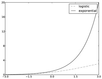
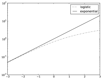
Figure 1: Exponential and logistic losses, plotted with linear and log-scale range.

Boosting determines some weighting $\lambda\in\mathbb{R}^{n}$ of the columns of $A$, which correspond to weak learners in $\mathcal{H}$. The (unnormalized) margin of example $i$ is thus $\left\langle-a_{i},\lambda\right\rangle=-\mathbf{e}_{i}^{\top}A\lambda$, where $\mathbf{e}_{i}$ is an indicator vector. (This negation is one notational inconvenience of making losses increasing.) Since the prediction on $x_{i}$ is $\mathds{1}[\sum_{j}\lambda_{j}h_{j}(x_{i})\geq 0]=\mathds{1}[y_{i}\left\langle a_{i},\lambda\right\rangle\leq 0]$, it follows that $A\lambda<\mathbf{0}_{m}$ (where $\mathbf{0}_{m}$ is the zero vector) implies a training error of zero. As such, boosting solves the minimization problem

$$\inf_{\lambda\in\mathbb{R}^{n}}\sum_{i=1}^{m}g(\left\langle a_{i},\lambda\right\rangle)=\inf_{\lambda\in\mathbb{R}^{n}}\sum_{i=1}^{m}g(\mathbf{e}_{i}^{\top}A\lambda)=\inf_{\lambda\in\mathbb{R}^{n}}f(A\lambda)=\inf_{\lambda\in\mathbb{R}^{n}}(f\circ A)(\lambda)=:\bar{f}_{A};$$ (2.1)

recall $f:\mathbb{R}^{m}\to\mathbb{R}$ is the convenience function $f(x)=\sum_{i}g((x)_{i})$, and in the present problem denotes the (unnormalized) empirical risk. $\bar{f}_{A}$ will denote the optimal objective value.

The infimum in (2.1) may well not be attainable. Suppose there exists $\lambda^{\prime}$ such that $A\lambda^{\prime}<\mathbf{0}_{m}$ (Theorem 5.1 will show that this is equivalent to the weak learning assumption). Then

$$0\leq\inf_{\lambda\in\mathbb{R}^{n}}f(A\lambda)\leq\inf_{c>0}f(A(c\lambda^{\prime}))=0.$$

On the other hand, for any $\lambda\in\mathbb{R}^{n}$, $f(A\lambda)>0$. Thus the infimum is never attainable when weak learnability holds.

The template boosting algorithm appears in Figure 2, formulated in terms of $f\circ A$ to make the connection to coordinate descent as clear as possible. To interpret the gradient terms, note that

$$(\nabla(f\circ A)(\lambda))_{j}=(A^{\top}\nabla f(A\lambda))_{j}=-\sum_{i=1}^{m}g^{\prime}(\left\langle a_{i},\lambda\right\rangle)h_{j}(x_{i})y_{i},$$

which is the expected negative correlation of $h_{j}$ with the target labels according to an unnormalized distribution with weights $g^{\prime}(\left\langle a_{i},\lambda\right\rangle)$. The stopping condition $\nabla(f\circ A)(\lambda)=\mathbf{0}_{m}$ means: either the distribution is degenerate (it is exactly zero), or every weak learner is uncorrelated with the target.

As such, Boost in Figure 2 represents an equivalent formulation of boosting, with one minor modification: the column (weak learner) selection has an absolute value. But note that this is the same as closing $\mathcal{H}$ under complementation (i.e., for any $h\in\mathcal{H}$, there exists $h^{(-)}$ with $h(x)=-h^{(-)}(x)$), which is assumed in many theoretical treatments of boosting.

Routine Boost. Input Convex function $f\circ A$. Output Approximate primal optimum $\lambda$. 1. Initialize $\lambda_{0}:=\mathbf{0}_{n}$. 2. For $t=1,2,\ldots$, while $\nabla(f\circ A)(\lambda_{t-1})\neq\mathbf{0}_{n}$: (a) Choose column (weak learner) $$j_{t}:=\operatornamewithlimits{argmax}_{j}|\nabla(f\circ A)(\lambda_{t-1})^{\top}\mathbf{e}_{j}|.$$ (b) Correspondingly, set descent direction $v_{t}\in\{\pm\mathbf{e}_{j_{t}}\}$; note $$v_{t}^{\top}\nabla(f\circ A)(\lambda_{t-1})=-\|\nabla(f\circ A)(\lambda_{t-1})\|_{\infty}.$$ (c) Find $\alpha_{t}$ via approximate solution to the line search $$\inf_{\alpha>0}(f\circ A)(\lambda_{t-1}+\alpha v_{t}).$$ (d) Update $\lambda_{t}:=\lambda_{t-1}+\alpha_{t}v_{t}$. 3. Return $\lambda_{t-1}$.

Figure 2: $l^{1}$ steepest descent (Boyd and Vandenberghe, 2004, Algorithm 9.4) of $f\circ A$.

In the case of the exponential loss and binary weak learners, the line search (when attainable) has a convenient closed form; but for other losses, and even with the exponential loss but with confidence-rated predictors, there may not be a closed form. As such, Boost only requires an approximate line search method. Appendix D details two mechanisms for this: an iterative method, which requires no knowledge of the loss function, and a closed form choice, which unfortunately requires some properties of the loss, which may be difficult to bound tightly. The iterative method provides a slightly worse guarantee, but is potentially more effective in practice; thus it will be used to produce all convergence rates in Section 6.

For simplicity, it is supposed that the best weak learner $j_{t}$ (or the approximation thereof encoded in $A$) can always be selected. Relaxing this condition is not without subtleties, but as discussed in Appendix E, there are ways to allow approximate selection without degrading the presented convergence rates.

As a final remark, consider the rows $\{-a_{i}\}_{1}^{m}$ of $-A$ as a collection of $m$ points in $\mathbb{R}^{n}$. Due to the form of $g$, Boost is therefore searching for a halfspace, parameterized by a vector $\lambda$, which contains all of these points. Sometimes such a halfspace may not exist, and $g$ applies a smoothly increasing penalty to points that are farther and farther outside it.

3 Dual Problem

Applying coordinate descent to (2.1) represents a valid interpretation of boosting, in the sense that the resulting algorithm Boost is equivalent to the original. However this representation loses the intuitive operation of boosting as generating distributions where the current predictor is highly erroneous, and requesting weak learners accurate on these tricky distributions. The dual problem will capture this.

In addition to illuminating the structure of boosting, the dual problem also possesses a major concrete contribution to the optimization behavior, and specifically the convergence rates: the dual optimum is always attainable.

The dual problem will make use of Fenchel conjugates (Hiriart-Urruty and Lemaréchal, 2001, Borwein and Lewis, 2000); for any function $h$, the conjugate is

$$h^{*}(\phi)=\sup_{x\in\textup{dom}(h)}\left\langle x,\phi\right\rangle-h(x).$$

Example 3.0.

The exponential loss $\exp(\cdot)$ has Fenchel conjugate

$$(\exp(\cdot))^{*}(\phi)=\begin{cases}\phi\ln(\phi)-\phi&\textup{when }\phi>0,\\ 0&\textup{when }\phi=0,\\ \infty&\textup{otherwise}.\end{cases}$$

The logistic loss $\ln(1+\exp(\cdot))$ has Fenchel conjugate

$$(\ln(1+\exp(\cdot)))^{*}(\phi)=\begin{cases}(1-\phi)\ln(1-\phi)+\phi\ln(\phi)&\textup{when }\phi\in(0,1),\\ 0&\textup{when }\phi\in\{0,1\},\\ \infty&\textup{otherwise}.\end{cases}$$

These conjugates are known respectively as the Boltzmann-Shannon and Fermi-Dirac entropies (see Borwein and Lewis, 2000, closing commentary, Section 3.3). Please see Figure 3 for a depiction.

Figure 3: Fenchel conjugates of exponential and logistic losses.

It further turns out that general members of $\mathbb{G}_{0}$ have a shape reminiscent of these two standard notions of entropy.

Lemma 3.0.

Let $g\in\mathbb{G}_{0}$ be given. Then $g^{*}$ is continuously differentiable on $\textup{int}(\textup{dom}(g^{*}))$, strictly convex, and either $\textup{dom}(g^{*})=[0,\infty)$ or $\textup{dom}(g^{*})=[0,b]$ where $b>0$. Furthermore, $g^{*}$ has the following form:

$$g^{*}(\phi)\in\begin{cases}\infty&\textup{when }\phi<0,\\ 0&\textup{when }\phi=0,\\ {\phantom{}}(-g(0),0)&\textup{when }\phi\in(0,g^{\prime}(0)),\\ -g(0)&\textup{when }\phi=g^{\prime}(0),\\ (-g(0),\infty]&\textup{when }\phi>g^{\prime}(0).\end{cases}$$

(The proof is in Appendix C.) There is one more object to present, the dual feasible set $\Phi_{A}$.

Definition 3.0.

For any $A\in\mathbb{R}^{m\times n}$, define the dual feasible set

$$\Phi_{A}:=\textup{Ker}(A^{\top})\cap\mathbb{R}^{m}_{+}$$

Consider any $\psi\in\Phi_{A}$. Since $\psi\in\textup{Ker}(A^{\top})$, this is a weighting of examples which decorrelates all weak learners from the target: in particular, for any primal weighting $\lambda\in\mathbb{R}^{n}$ over weak learners, $\psi^{\top}A\lambda=0$. And since $\psi\in\mathbb{R}^{m}_{+}$, all coordinates are nonnegative, so in the case that $\psi\neq\{\mathbf{0}_{m}\}$, this vector may be renormalized into a distribution over examples. The case $\Phi_{A}=\{\mathbf{0}_{m}\}$ is an extremely special degeneracy: it will be shown to encode the scenario of weak learnability.

Theorem 3.1.

For any $A\in\mathbb{R}^{m\times n}$ and $g\in\mathbb{G}_{0}$ with $f(x)=\sum_{i}g((x)_{i})$,

$$\inf\left\{f(A\lambda):\lambda\in\mathbb{R}^{n}\right\}=\sup\left\{-f^{*}(\psi):\psi\in\Phi_{A}\right\},$$ (3.2)

where $f^{*}(\phi)=\sum_{i=1}^{m}g^{*}((\phi)_{i})$. The right hand side is the dual problem, and moreover the dual optimum, denoted $\psi_{A}^{f}$, is unique and attainable.

(The proof uses routine techniques from convex analysis, and is deferred to Section G.2.)

The definition of $\Phi_{A}$ does not depend on any specific $g\in\mathbb{G}_{0}$; this choice was made to provide general intuition on the structure of the problem for the entire family of losses. Note however that this will cause some problems later. For instance, with the logistic loss, the vector with every value two, i.e. $2\cdot\mathbf{1}_{m}$, has objective value $-f^{*}(2\cdot\mathbf{1}_{m})=-\infty$. In a sense, there are points in $\Phi_{A}$ which are not really candidates for certain losses, and this fact will need adjustment in some convergence rate proofs.

Remark 3.2.

Finishing the connection to maximum entropy, for any $g\in\mathbb{G}_{0}$, by Section 3, the optimum of the unconstrained problem is $g^{\prime}(0)\mathbf{1}_{m}$, a rescaling of the uniform distribution. But note that $\nabla f(A\lambda_{0})=\nabla f(\mathbf{0}_{m})=g^{\prime}(0)\mathbf{1}_{m}$: that is, the initial dual iterate is the unconstrained optimum! Let $\phi_{t}:=\nabla f(A\lambda_{t})$ denote the $t^{\textup{th}}$ dual iterate; since $\nabla f^{*}(\nabla f(x))=x$ (cf. Section B.2), then for any $\psi\in\Phi_{A}\subseteq\textup{Ker}(A^{\top})$,

$$\left\langle\nabla f^{*}(\phi_{t}),\psi\right\rangle=\left\langle A\lambda_{t},\psi\right\rangle=\left\langle\lambda_{t},A^{\top}\psi\right\rangle=0.$$

This allows the dual optimum to be rewritten as

$$\psi_{A}^{f} =\operatornamewithlimits{argmin}_{\psi\in\Phi_{A}}f^{*}(\psi)$$

$$=\operatornamewithlimits{argmin}_{\psi\in\Phi_{A}}f^{*}(\psi)-f^{*}(\phi_{t})-\left\langle\nabla f^{*}(\phi_{t}),\psi-\phi_{t}\right\rangle;$$

that is, the dual optimum $\psi^{f}_{A}$ is the Bregman projection (according to $f^{*}$) onto $\Phi_{A}$ of any dual iterate $\phi_{t}=\nabla f(A\lambda_{t})$. In particular, $\psi^{f}_{A}$ is the Bregman projection onto the feasible set of the unconstrained optimum $\phi_{0}=\nabla f(A\lambda_{0})$!

The connection to Bregman divergences runs deep; in fact, mirroring the development of Boost as “compiling out” the dual variables in the classical boosting presentation, it is possible to compile out the primal variables, producing an algorithm using only dual variables, meaning distributions over examples. This connection has been explored extensively (Kivinen and Warmuth, 1999, Collins et al., 2002).

Remark 3.2.

It may be tempting to use Theorem 3.1 to produce a stopping condition; that is, if for a supplied $\epsilon>0$, a primal iterate $\lambda^{\prime}$ and dual feasible $\psi^{\prime}\in\Phi_{A}$ can be found satisfying $f(A\lambda^{\prime})+f^{*}(\psi^{\prime})\leq\epsilon$, Boost may terminate with the guarantee $f(A\lambda^{\prime})-\bar{f}_{A}\leq\epsilon$.

Unfortunately, it is unclear how to produce dual iterates (excepting the trivial $\mathbf{0}_{m}$). If $\textup{Ker}(A^{\top})$ can be computed, it suffices to $l^{2}$ project $\nabla f(A\lambda_{t})$ onto this subspace. In general however, not only is $\textup{Ker}(A^{\top})$ painfully expensive to compute, this computation does not at all fit the oracle model of boosting, where access to $A$ is obscured. (What is $\textup{Ker}(A^{\top})$ when the weak learning oracle learns a size-bounded decision tree?)

In fact, noting that the primal-dual relationship from (3.2) can be written

$$\inf\left\{f(\Lambda):\Lambda\in\textup{Im}(A)\right\}=\sup\left\{-f^{*}(\Psi):\Psi\in\textup{Ker}(A^{\top})=\textup{Im}(A)^{\perp}\right\}$$

(since $\textup{dom}(f^{*})\subseteq\mathbb{R}^{m}_{+}$ encodes the orthant constraint), the standard oracle model gives elements of $\textup{Im}(A)$, but what is needed in the dual is an oracle for $\textup{Ker}(A^{\top})=\textup{Im}(A)^{\perp}$.

4 Generalized Weak Learning Rate

The weak learning rate was critical to the original convergence analysis of AdaBoost, providing a handle on the progress of the algorithm. But to be useful, this value must be positive, which was precisely the condition granted by the weak learning assumption. This section will generalize the weak learning rate into a quantity which can be made positive for any boosting instance.

Note briefly that this manuscript will differ slightly from the norm in that weak learning will be a purely sample-specific concept. That is, the concern here is convergence in empirical risk, and all that matters is the sample $\mathcal{S}=\{(x_{i},y_{i})\}_{1}^{m}$, as encoded in $A$; it doesn’t matter if there are wild points outside this sample, because the algorithm has no access to them.

This distinction has the following implication. The usual weak learning assumption states that there exists no uncorrelating distribution over the input space. This of course implies that any training sample $\mathcal{S}$ used by the algorithm will also have this property; however, it suffices that there is no distribution over the input sample $\mathcal{S}$ which uncorrelates the weak learners from the target.

Returning to task, the weak learning assumption posits the existence of a positive constant, the weak learning rate $\gamma$, which lower bounds the correlation of the best weak learner with the target for any distribution. Stated in terms of the matrix $A$,

$$0<\gamma=\inf_{\begin{subarray}{c}\phi\in\mathbb{R}^{m}_{+}\\ \|\phi\|=1\end{subarray}}\max_{j\in[n]}\left|\sum_{i=1}^{m}(\phi)_{i}y_{i}h_{j}(x_{i})\right|=\inf_{\begin{subarray}{c}\phi\in\mathbb{R}^{m}_{+}\setminus\{\mathbf{0}_{m}\}\end{subarray}}\frac{\|A^{\top}\phi\|_{\infty}}{\|\phi\|_{1}}=\inf_{\begin{subarray}{c}\phi\in\mathbb{R}^{m}_{+}\setminus\{\mathbf{0}_{m}\}\end{subarray}}\frac{\|A^{\top}\phi\|_{\infty}}{\|\phi-\mathbf{0}_{m}\|_{1}}.$$ (4.1)

Proposition 4.1.

A boosting instance is weak learnable iff $\Phi_{A}=\{\mathbf{0}_{m}\}$.

Proof.

Suppose $\Phi_{A}=\{\mathbf{0}_{m}\}$; since the first infimum in (4.1) is of a continuous function over a compact set, it has some minimizer $\phi^{\prime}$. But $\|\phi^{\prime}\|_{1}=1$, meaning $\phi^{\prime}\not\in\Phi_{A}$, and so $\|A^{\top}\phi^{\prime}\|_{\infty}>0$. On the other hand, if $\Phi_{A}\neq\{\mathbf{0}_{m}\}$, take any $\phi^{\prime\prime}\in\Phi_{A}\setminus\{\mathbf{0}_{m}\}$; then

$$0\leq\gamma=\inf_{\begin{subarray}{c}\phi\in\mathbb{R}^{m}_{+}\setminus\{\mathbf{0}_{m}\}\end{subarray}}\frac{\|A^{\top}\phi\|_{\infty}}{\|\phi\|_{1}}\leq\frac{\|A^{\top}\phi^{\prime\prime}\|_{\infty}}{\|\phi^{\prime\prime}\|_{1}}=0.\qed$$

Following this connection, the first way in which the weak learning rate is modified is to replace $\{\mathbf{0}_{m}\}$ with the dual feasible set $\Phi_{A}=\textup{Ker}(A^{\top})\cap\mathbb{R}^{m}_{+}$. For reasons that will be sketched shortly, but fully dealt with only in Section 6, it is necessary to replace $\mathbb{R}^{m}_{+}$ with a more refined choice $S$.

Definition 4.1.

Given a matrix $A\in\mathbb{R}^{m\times n}$ and a set $S\subseteq\mathbb{R}^{m}$, define

$$\gamma(A,S):=\inf\left\{\frac{\|A^{\top}\phi\|_{\infty}}{\inf_{\psi\in S\cap\textup{Ker}(A^{\top})}\|\phi-\psi\|_{1}}:\phi\in S\setminus\textup{Ker}(A^{\top})\right\}.$$

First note that in the scenario of weak learnability (i.e., $\Phi_{A}=\{\mathbf{0}_{m}\}$ by Section 4), the choice $S=\mathbb{R}^{m}_{+}$ allows the new notion to exactly cover the old one: $\gamma(A,\mathbb{R}^{m}_{+})=\gamma$.

To get a better handle on the meaning of $S$, first define the following projection and distance notation to a closed convex nonempty set $C$, where in the case of non-uniqueness ($l^{1}$ and $l^{\infty}$), some arbitrary choice is made:

$$\mathsf{P}^{p}_{C}(x)\in\operatornamewithlimits{Argmin}_{y\in C}\|y-x\|_{p}, \mathsf{D}^{p}_{C}(x)=\|x-\mathsf{P}^{p}_{C}(x)\|_{p}.$$

Suppose, for some $t$, that $\nabla f(A\lambda_{t})\in S\setminus\textup{Ker}(A^{\top})$; then the infimum within $\gamma(A,S)$ may be instantiated with $\nabla f(A\lambda_{t})$, yielding

$$\gamma(A,S)=\inf_{\phi\in S\setminus\textup{Ker}(A^{\top})}\frac{\|A^{\top}\phi\|_{\infty}}{\|\phi-\mathsf{P}^{1}_{S\cap\textup{Ker}(A^{\top})}(\phi)\|_{1}}\leq\frac{\|A^{\top}\nabla f(A\lambda_{t})\|_{\infty}}{\|\nabla f(A\lambda_{t})-\mathsf{P}^{1}_{S\cap\textup{Ker}(A^{\top})}(\nabla f(A\lambda_{t}))\|_{1}}.$$ (4.2)

Rearranging this,

$$\gamma(A,S)\left\|\nabla f(A\lambda_{t})-\mathsf{P}^{1}_{S\cap\textup{Ker}(A^{\top})}(\nabla f(A\lambda_{t}))\right\|_{1}\leq\|A^{\top}\nabla f(A\lambda_{t})\|_{\infty}.$$ (4.3)

This is helpful because the right hand side appears in standard guarantees for single-step progress in descent methods. Meanwhile, the left hand side has reduced the influence of $A$ to a single number, and the normed expression is the distance to a restriction of dual feasible set, which will converge to zero if the infimum is to be approached, so long as this restriction contains the dual optimum.

This will be exactly the approach taken in this manuscript; indeed, the first step towards convergence rates, Proposition 7, will use exactly the upper bound in (4.3). The detailed work that remains is then dealing with the distance to the dual feasible set. The choice of $S$ will be made to facilitate the production of these bounds, and will depend on the optimization structure revealed in Section 5.

In order for these expressions to mean anything, $\gamma(A,S)$ must be positive.

Theorem 4.4.

Let matrix $A\in\mathbb{R}^{m\times n}$ and polyhedron $S\subseteq\mathbb{R}^{m}$ be given with $S\setminus\textup{Ker}(A^{\top})\neq\emptyset$ and $S\cap\textup{Ker}(A^{\top})\neq\emptyset$. Then $\gamma(A,S)>0$.

The proof, material on other generalizations of $\gamma$, and discussion on the polyhedrality of $S$ can all be found in Appendix F.

As a final connection, since $A^{\top}\mathsf{P}^{1}_{S\cap\textup{Ker}(A^{\top})}(\phi)=\mathbf{0}_{n}$, note that

$$\gamma(A,S)=\inf_{\phi\in S\setminus\textup{Ker}(A^{\top})}\frac{\|A^{\top}\phi\|_{\infty}}{\|\phi-\mathsf{P}^{1}_{S\cap\textup{Ker}(A^{\top})}(\phi)\|_{1}}=\inf_{\phi\in S\setminus\textup{Ker}(A^{\top})}\frac{\|A^{\top}(\phi-\mathsf{P}^{1}_{S\cap\textup{Ker}(A^{\top})}(\phi))\|_{\infty}}{\|\phi-\mathsf{P}^{1}_{S\cap\textup{Ker}(A^{\top})}(\phi)\|_{1}}.$$

In this way, $\gamma(A,S)$ resembles a Lipschitz constant, reflecting the effect of $A$ on elements of the dual, relative to the dual feasible set.

5 Optimization Structure

The scenario of weak learnability translates into a simple condition on the dual feasible set: the dual feasible set is the origin (in symbols, $\Phi_{A}=\textup{Ker}(A^{\top})\cap\mathbb{R}^{m}_{+}=\{\mathbf{0}_{m}\}$). And how about attainability—is there a simple way to encode this problem in terms of the optimization problem?

This section will identify the structure of the boosting optimization problem both in terms of the primal and dual problems, first studying the scenarios of weak learnability and attainability, and then showing that general instances can be decomposed into these two.

There is another behavior which will emerge through this study, motivated by the following question. The dual feasible set $\Phi_{A}=\textup{Ker}(A^{\top})\cap\mathbb{R}^{m}_{+}$ is the set of nonnegative weightings of examples under which every weak learner (every column of $A$) has zero correlation; what is the support of these weightings?

Definition 5.0.

$H(A)$ denotes the hard core of $A$: the collection of examples which receive positive weight under some dual feasible point, a distribution upon which no weak learner is correlated with the target. Symbolically,

$$H(A):=\{i\in[m]:\exists\psi\in\Phi_{A},(\psi)_{i}>0\}.$$

One case has already been considered; as established in Section 4, weak learnability is equivalent to $\Phi_{A}=\{\mathbf{0}_{m}\}$, which in turn is equivalent to $|H(A)|=0$. But it will turn out that other possibilities for $H(A)$ also have direct relevance to the behavior of Boost. Indeed, contrasted with the primal and dual problems and feasible sets, $H(A)$ will provide a conceptually simple, discrete object with which to comprehend the behavior of boosting.

5.1 Weak Learnability

The following theorem establishes four equivalent formulations of weak learnability.

Theorem 5.1.

For any $A\in\mathbb{R}^{m\times n}$ and $g\in\mathbb{G}_{0}$ the following conditions are equivalent:

1. $\exists\lambda\in\mathbb{R}^{n}\centerdot A\lambda\in\mathbb{R}^{m}_{--}$,

2. $\inf_{\lambda\in\mathbb{R}^{n}}f(A\lambda)=0$,

3. $\psi_{A}^{f}=\mathbf{0}_{m}$,

4. $\Phi_{A}=\{\mathbf{0}_{m}\}$.

First note that (0.4) indicates (via Section 4) this is indeed the weak learnability setting, equivalently $|H(A)|=0$.

Recall the earlier discussion of boosting as searching for a halfspace containing the points $\{-a_{i}\}_{1}^{m}=\{-\mathbf{e}_{i}^{\top}A\}_{1}^{m}$; property (0.1) encodes precisely this statement, and moreover that there exists such a halfspace with these points interior to it. Note that this statement also encodes the margin separability equivalence of weak learnability due to Shalev-Shwartz and Singer (2008); specifically, if labels are bounded away from 0 and each point $-a_{i}$ (row of $-A$) is replaced with $-y_{i}a_{i}$, the definition of $A$ grants that positive examples will land on one side of the hyperplane, and negative examples on the other.

The two properties (0.4) and (0.1) can be interpreted geometrically, as depicted in Figure 4: the dual feasibility statement is that no convex combination of $\{-a_{i}\}_{1}^{m}$ will contain the origin.

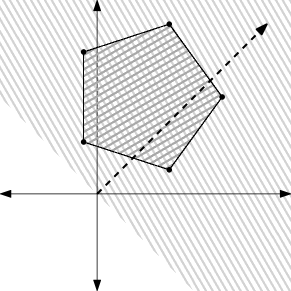
Figure 4: Geometric view of the primal and dual problem, under weak learnability. The vertices of the pentagon denote the points $\{-a_{i}\}_{1}^{m}$. The arrow, denoting $\lambda$ in (0.1), defines a homogeneous halfspace containing these points; on the other hand, their convex hull does not contain the origin. Please see Theorem 5.1 and its discussion.

Next, (0.2) is the (error part of the) usual strong PAC guarantee (Schapire, 1990): weak learnability entails that the training error will go to zero. And, as must be the case when $\Phi_{A}=\{\mathbf{0}_{m}\}$, property (0.3) provides that $\psi_{A}^{f}=\mathbf{0}_{m}$.

Proof of Theorem 5.1.

($\eqref{eq:gordan:a}\implies\eqref{eq:gordan:b}$) Let $\bar{\lambda}\in\mathbb{R}^{n}$ be given with $A\bar{\lambda}\in\mathbb{R}^{m}_{--}$, and let any increasing sequence $\{c_{i}\}_{1}^{\infty}\uparrow\infty$ be given. Then, since $f>0$ and $\lim_{x\to-\infty}g(x)=0$,

$$\inf_{\lambda}f(A\lambda)\leq\lim_{i\to\infty}f(c_{i}A\bar{\lambda})=0\leq\inf_{\lambda}f(A\lambda).$$

($\eqref{eq:gordan:b}\implies\eqref{eq:gordan:c}$) The point $\mathbf{0}_{m}$ is always dual feasible, and

$$\inf_{\lambda}f(A\lambda)=0=-f^{*}(\mathbf{0}_{m}).$$

Since the dual optimum is unique (Theorem 3.1), $\psi_{A}^{f}=\mathbf{0}_{m}$.

($\eqref{eq:gordan:c}\implies\eqref{eq:gordan:d}$) Suppose there exists $\psi\in\Phi_{A}$ with $\psi\neq\mathbf{0}_{m}$. Since $-f^{*}$ is continuous and increasing along every positive direction at $\mathbf{0}_{m}=\psi_{A}^{f}$ (see Section 3 and Lemma 16), there must exist some tiny $\tau>0$ such that $-f^{*}(\tau\psi)>-f^{*}(\psi_{A}^{f})$, contradicting the selection of $\psi_{A}^{f}$ as the unique optimum.

($\eqref{eq:gordan:d}\implies\eqref{eq:gordan:a}$) This case is directly handled by Gordan’s theorem (cf. Theorem B.1). ∎

5.2 Attainability

For strictly convex functions, there is a nice characterization of attainability, which will require the following definition.

Definition 1 (cf. Hiriart-Urruty and Lemaréchal (2001, Definition B.3.2.5)).

A closed convex function $h$ is called 0-coercive when all level sets are compact. (That is, for any $\alpha\in\mathbb{R}$, the set $\{x:f(x)\leq\alpha\}$ is compact.)

Proposition 2.

Suppose $h$ is differentiable, strictly convex, and $\textup{dom}(h)=\mathbb{R}^{m}$. Then $\inf_{x}h(x)$ is attainable iff $h$ is 0-coercive.

Note that 0-coercivity means the domain of the infimum in (2.1) can be restricted to a compact set, and attainability in turn follows just from properties of minimization of continuous functions on compact sets. It is the converse which requires some structure; the proof however is unilluminating and deferred to Section G.3.

Armed with this notion, it is now possible to build an attainability theory for $f\circ A$. Some care must be taken with the above concepts, however; note that while $f$ is strictly convex, $f\circ A$ need not be (for instance, if there exist nonzero elements of $\textup{Ker}(A)$, then moving along these directions does not change the objective value). Therefore, 0-coercivity statements will refer to the function

$$(f+\iota_{\textup{Im}(A)})(x)=\begin{cases}f(x)&\textup{when }x\in\textup{Im}(A),\\ \infty&\textup{otherwise}.\end{cases}$$

This function is effectively taking the epigraph of $f$, and intersecting it with a slice representing $\textup{Im}(A)=\{A\lambda:\lambda\in\mathbb{R}^{n}\}$, the set of points considered by the algorithm. As such, it is merely a convenient way of dealing with $\textup{Ker}(A)$ as discussed above.

Theorem 5.2.

For any $A\in\mathbb{R}^{m\times n}$ and $g\in\mathbb{G}_{0}$, the following conditions are equivalent:

1. $\forall\lambda\in\mathbb{R}^{n}\centerdot A\lambda\not\in\mathbb{R}^{m}_{-}\setminus\{\mathbf{0}_{m}\}$,

2. $f+\iota_{\textup{Im}(A)}$ is 0-coercive,

3. $\psi_{A}^{f}\in\mathbb{R}^{m}_{++}$,

4. $\Phi_{A}\cap\mathbb{R}^{m}_{++}\neq\emptyset$.

Following the discussion above, (2.2) is the desired attainability statement.

Next, note that (2.4) is equivalent to the expression $|H(A)|=m$, i.e. there exists a distribution with positive weight on all examples, upon which every weak learner is uncorrelated. The forward direction is direct from the existence of a single $\psi\in\Phi_{A}\cap\mathbb{R}^{m}_{++}$. For the converse, note that the $\psi_{i}$ corresponding to each $i\in H(A)$ can be combined into $\psi=\sum_{i}\psi_{i}\in\textup{Ker}(A^{\top})\cap\mathbb{R}^{m}_{++}$ (since $\textup{Ker}(A^{\top})$ is a subspace).

For a geometric interpretation, consider (2.1) and (2.4). The first says that any halfspace containing some $-a_{i}$ within its interior must also fail to contain some $-a_{j}$ (with $i\neq j$). (Property (2.1) also allows for the scenario that no valid enclosing halfspace exists, i.e. $\lambda=\mathbf{0}_{n}$.) The latter states that the origin $\mathbf{0}_{m}$ is contained within a positive convex combination of $\{-a_{i}\}_{1}^{m}$ (alternatively, the origin is within the relative interior of these points). These two scenarios appear in Figure 5.

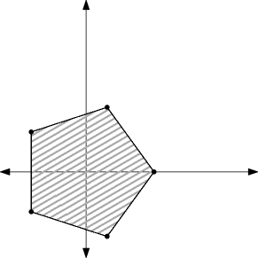
Figure 5: Geometric view of the primal and dual problem, under attainability. Once again, the $\{-a_{i}\}_{1}^{m}$ are the vertices of the pentagon. This time, no (closed) homogeneous halfspace containing all the points will contain one strictly, and the relative interior of the pentagon contains the origin. Please see Theorem 5.2 and its discussion.

Finally, note (2.3): it is not only the case that there are dual feasible points fully interior to $\mathbb{R}^{m}_{+}$, but furthermore the dual optimum is also interior. This will be crucial in the convergence rate analysis, since it will allow the dual iterates to never be too small.

Proof of Theorem 5.2.

($\eqref{eq:stiemke:a}\implies\eqref{eq:stiemke:b}$) Let $d\in\mathbb{R}^{m}\setminus\{\mathbf{0}_{m}\}$ and $\lambda\in\mathbb{R}^{n}$ be arbitrary. To show 0-coercivity, it suffices (Hiriart-Urruty and Lemaréchal, 2001, Proposition B.3.2.4.iii) to show

$$\lim_{t\to\infty}\frac{f(A\lambda+td)+\iota_{\textup{Im}(A)}(A\lambda+td)-f(A\lambda)}{t}>0.$$ (5.3)

If $d\not\in\textup{Im}(A)$ (and $t>0$), then $\iota_{\textup{Im}(A)}(A\lambda+td)=\infty$. Suppose $d\in\textup{Im}(A)$; by (2.1), since $d\neq\mathbf{0}_{m}$, then $d\not\in\mathbb{R}^{m}_{-}$, meaning there is at least one positive coordinate $j$. But then, since $g>0$ and $g$ is convex,

$$\eqref{eq:stiemke:helperdog:1} \geq\lim_{t\to\infty}\frac{g(\mathbf{e}_{j}^{\top}(A\lambda+td))-f(A\lambda)}{t}$$

$$\geq\lim_{t\to\infty}\frac{g(\mathbf{e}_{j}^{\top}A\lambda)+td_{j}g^{\prime}(\mathbf{e}_{j}^{\top}A\lambda)-f(A\lambda)}{t}$$

$$=d_{j}g^{\prime}(\mathbf{e}_{j}^{\top}A\lambda),$$

which is positive by the selection of $d_{j}$ and since $g^{\prime}>0$.

($\eqref{eq:stiemke:b}\implies\eqref{eq:stiemke:c}$) Since the infimum is attainable, designate any $\bar{\lambda}$ satisfying $\inf_{\lambda}f(A\lambda)=f(A\bar{\lambda})$ (note, although $f$ is strictly convex, $f\circ A$ need not be, thus uniqueness is not guaranteed!). The optimality conditions of Fenchel problems may be applied, meaning $\psi_{A}^{f}=\nabla f(A\bar{\lambda})$, which is interior to $\mathbb{R}^{m}_{+}$ since $\nabla f\in\mathbb{R}^{m}_{++}$ everywhere (cf. Lemma 16). (For the optimality conditions, see Borwein and Lewis (2000, Exercise 3.3.9.f), with a negation inserted to match the negation inserted within the proof of Theorem 3.1.)

($\eqref{eq:stiemke:c}\implies\eqref{eq:stiemke:d}$) This holds since $\Phi_{A}\supseteq\{\psi_{A}^{f}\}$ and $\psi_{A}^{f}\in\mathbb{R}^{m}_{++}$.

($\eqref{eq:stiemke:d}\implies\eqref{eq:stiemke:a}$) This case is directly handled by Stiemke’s Theorem (cf. Theorem B.4). ∎

5.3 General Setting

So far, the scenarios of weak learnability and attainability corresponded to the extremal hard core cases of $|H(A)|\in\{0,m\}$. The situation in the general setting $1\leq|H(A)|\leq m-1$ is basically as good as one could hope for: it interpolates between the two extremal cases.

As a first step, partition $A$ into two submatrices according to $H(A)$.

Definition 3.

Partition $A\in\mathbb{R}^{m\times n}$ by rows into two matrices $A_{0}\in\mathbb{R}^{m_{0}\times n}$ and $A_{+}\in\mathbb{R}^{m_{+}\times n}$, where $A_{+}$ has rows corresponding to $H(A)$, and $m_{+}=|H(A)|$. For convenience, permute the examples so that

$$A=\left[\begin{smallmatrix}A_{0}\\ A_{+}\end{smallmatrix}\right].$$

(This merely relabels the coordinate axes, and does not change the optimization problem.) Note that this decomposition is unique, since $H(A)$ is uniquely specified.

As a first consequence, this partition cleanly decomposes the dual feasible set $\Phi_{A}$ into $\Phi_{A_{0}}$ and $\Phi_{A_{+}}$.

Proposition 4.

For any $A\in\mathbb{R}^{m\times n}$, $\Phi_{A_{0}}=\{\mathbf{0}_{m_{0}}\}$, $\Phi_{A_{+}}\cap\mathbb{R}^{m_{+}}_{++}\neq\emptyset$, and

$$\Phi_{A}=\Phi_{A_{0}}\times\Phi_{A_{+}}.$$

Furthermore, no other partition of $A$ into $B_{0}\in\mathbb{R}^{z\times n}$ and $B_{+}\in\mathbb{R}^{p\times n}$ satisfies these properties.

Proof.

It must hold that $\Phi_{A_{0}}=\{\mathbf{0}_{m_{0}}\}$, since otherwise there would exist $\psi\in\textup{Ker}(A_{0}^{\top})\cap\mathbb{R}^{m_{0}}_{+}$ with $\psi\neq\mathbf{0}_{m_{0}}$, which could be extended to $\psi^{\prime}=\psi\times\mathbf{0}_{m_{+}}\in\Phi_{A}$ and the positive coordinate of $\psi$ could be added to $H(A)$, contradicting the construction of $H(A)$ as including all such rows.

The property $\Phi_{A_{+}}\cap\mathbb{R}^{m_{+}}_{++}\neq\emptyset$ was proved in the discussion of Theorem 5.2: simply add together, for each $i\in H(A)$, the $\psi_{i}$’s corresponding to positive weight on $i$.

For the decomposition, note first that certainly every $\psi\in\Phi_{A_{0}}\times\Phi_{A_{+}}$ satisfies $\psi\in\Phi_{A}$. Now suppose contradictorily that there exists $\psi^{\prime}\in\Phi_{A}\setminus(\Phi_{A_{0}}\times\Phi_{A_{+}})$. There must exist $j\in[m]\setminus H(A)$ with $(\psi^{\prime})_{j}>0$, since otherwise $\psi^{\prime}\in\{\mathbf{0}_{z}\}\times\Phi_{A_{+}}$; but that means $j$ should have been included in $H(A)$, a contradiction.

For the uniqueness property, suppose some other $B_{0},B_{+}$ is given, satisfying the desired properties. It is impossible that some $a_{i}\in B_{+}$ is not in $H(A)$, since any $\psi\in\Phi_{B_{+}}$ can be extended to $\psi^{\prime}\in\Phi_{A}$ with positive weight on $i$, and thus is included in $H(A)$ by definition. But the other case with $i\in H(A)$ but $a_{i}\in B_{0}$ is equally untenable, since the corresponding measure $\psi_{i}$ is in $\Phi_{A}$ but not in $\Phi_{B_{0}}\times\Phi_{B_{+}}$. ∎

The main result of this section will have the same two main ingredients as Proposition 4:

• The full boosting instance may be uniquely decomposed into two pieces, $A_{0}$ and $A_{+}$, each of which individually behave like the weak learnability and attainability scenarios.

• The subinstances have a somewhat independent effect on the full instance.

Theorem 5.4.

Let $g\in\mathbb{G}_{0}$ and $A\in\mathbb{R}^{m\times n}$ be given. Let $B_{0}\in\mathbb{R}^{z\times n}$, $B_{+}\in\mathbb{R}^{p\times n}$ be any partition of $A$ by rows. The following conditions are equivalent:

1. $\exists\lambda\in\mathbb{R}^{n}\centerdot B_{0}\lambda\in\mathbb{R}^{z}_{--}\land B_{+}\lambda=\mathbf{0}_{p}$     and     $\forall\lambda\in\mathbb{R}^{n}\centerdot B_{+}\lambda\not\in\mathbb{R}^{p}_{-}\setminus\{\mathbf{0}_{p}\}$,

2. $\inf_{\lambda\in\mathbb{R}^{n}}f(A\lambda)=\inf_{\lambda\in\mathbb{R}^{n}}f(B_{+}\lambda)$,     and     $\inf_{\lambda\in\mathbb{R}^{n}}f(B_{0}\lambda)=0$,
   and     $f+\iota_{\textup{Im}(B_{+})}$ is 0-coercive,

3. $\psi_{A}^{f}=\left[\begin{smallmatrix}\psi_{B_{0}}^{f}\\ \psi_{B_{+}}^{f}\end{smallmatrix}\right]$     with     $\psi_{B_{0}}^{f}=\mathbf{0}_{z}$     and     $\psi_{B_{+}}^{f}\in\mathbb{R}^{p}_{++}$,

4. $\Phi_{B_{0}}=\{\mathbf{0}_{z}\}$,     and     $\Phi_{B_{+}}\cap\mathbb{R}^{p}_{++}\neq\emptyset$,     and     $\Phi_{A}=\Phi_{B_{0}}\times\Phi_{B_{+}}$.

Stepping through these properties, notice that (4.4) mirrors the expression in Proposition 4. But that proposition also granted that this representation was unique, thus only one partition of $A$ satisfies the above properties, namely $A_{0},A_{+}$. Since this Theorem is stated as a series of equivalences, any one of these properties can in turn be used to identify the hard core set $H(A)$.

To continue with geometric interpretations, notice that (4.1) states that there exists a halfspace strictly containing those points in $[m]\setminus H(A)$, with all points of $H(A)$ on its boundary; furthermore, trying to adjust this halfspace to contain elements of $H(A)$ will place others outside it. With regards to the geometry of the dual feasible set as provided by (4.4), the origin is within the relative interior of the points corresponding to $H(A)$, however the convex hull of the other $m-|H(A)|$ points can not contain the origin. Furthermore, if the origin is written as a convex combination of all points, this combination must place zero weight on the points with indices $[m]\setminus H(A)$. This scenario is depicted in Figure 6.

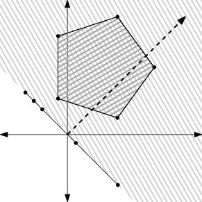
Figure 6: Geometric view of the primal and dual problem in the general case. There is a closed homogeneous halfspace containing the points $\{-a_{i}\}_{1}^{m}$, where the hard core lies on the halfspace boundary, and the other points are within its interior; moreover, there does not exist a closed homogeneous halfspace containing all points but with strict containment on a point in the hard core. Finally, although the origin is in the convex hull of $\{-a_{i}\}_{1}^{m}$, any such convex combination places zero weight on points outside the hard core. Please see Theorem 5.4 and its discussion.

In properties (4.2) and (4.3), $B_{0}$ mirrors the behavior of weakly learnable instances in Theorem 5.1, and analogously $B_{+}$ follows instances with minimizers from Theorem 5.2. The interesting addition, as discussed above, is the independence of these components: (4.2) provides that the infimum of the combined problem is the sum of the infima of the subproblems, while (4.3) provides that the full dual optimum may be obtained by concatenating the subproblems’ dual optima.

Proof of Theorem 5.4.

($\eqref{eq:decomp:a}\implies\eqref{eq:decomp:b}$) Let $\bar{\lambda}$ be given with $B_{0}\bar{\lambda}\in\mathbb{R}^{z}_{--}$ and $B_{+}\bar{\lambda}=\mathbf{0}_{p}$, and let $\{c_{i}\}_{1}^{\infty}\uparrow\infty$ be an arbitrary sequence increasing without bound. Lastly, let $\{\lambda_{i}\}_{1}^{\infty}$ be a minimizing sequence for $\inf_{\lambda}f(B_{+}\lambda)$. Then

$$\inf_{\lambda}f(B_{+}\lambda) =\lim_{i\to\infty}\left(f(B_{+}\lambda_{i})+f(c_{i}B_{0}\bar{\lambda})\right)\geq\inf_{\lambda}f(A\lambda)$$

$$=\inf_{\lambda}(f(B_{+}\lambda)+f(B_{0}\lambda))\geq\inf_{\lambda}f(B_{+}\lambda),$$

which used the fact that $f(B_{0}\lambda)\geq 0$ since $f\geq 0$. And since the chain of inequalities starts and ends the same, it must be a chain of equalities, which means $\inf_{\lambda}f(B_{0}\lambda)=0$. To show 0-coercivity of $f+\iota_{\textup{Im}(B_{+})}$, note the second part of $\eqref{eq:decomp:a}$ is one of the conditions of Theorem 5.2.

($\eqref{eq:decomp:b}\implies\eqref{eq:decomp:c}$) First, by Theorem 5.1, $\inf_{\lambda}f(B_{0}\lambda)=0$ means $\psi_{B_{0}}^{f}=\mathbf{0}_{z}$ and $\Phi_{B_{0}}=\{\mathbf{0}_{z}\}$. Thus

$$-f^{*}(\psi_{A}^{f}) =\sup_{\psi\in\Phi_{A}}-f^{*}(\psi)$$

$$=\sup\left\{-f^{*}(\psi_{z})-f^{*}(\psi_{p}):\psi_{z}\in\mathbb{R}^{z}_{+},\psi_{p}\in\mathbb{R}^{p}_{+},B_{0}^{\top}\psi_{z}+B_{+}^{\top}\psi_{p}=\mathbf{0}_{n}\right\}$$

$$\geq\sup_{\psi_{z}\in\Phi_{B_{0}}}-f^{*}(\psi_{z})+\sup_{\psi_{p}\in\Phi_{B_{+}}}-f^{*}(\psi_{p})$$

$$=0-f^{*}(\psi_{B_{+}}^{f})=\inf_{\lambda\in\mathbb{R}^{n}}f(B_{+}\lambda)=\inf_{\lambda\in\mathbb{R}^{n}}f(A\lambda)=-f^{*}(\psi_{A}^{f}).$$

Combining this with $f^{*}(x)=\sum_{i}g((x)_{i})$ and $g^{*}(0)=0$ (cf. Sections 3 and 3.1), $f^{*}(\psi_{A}^{f})=f^{*}(\psi_{B_{+}}^{f})=f^{*}(\left[\begin{smallmatrix}\psi_{B_{0}}^{f}\\ \psi_{B_{+}}^{f}\end{smallmatrix}\right])$. But Theorem 3.1 shows $\psi_{A}^{f}$ was unique, which gives the result. And to obtain $\psi_{B_{+}}^{f}\in\mathbb{R}^{p}_{++}$, use Theorem 5.2 with the 0-coercivity of $f+\iota_{\textup{Im}(B_{+})}$.

($\eqref{eq:decomp:c}\implies\eqref{eq:decomp:d}$) Since $\psi_{B_{0}}^{f}=\mathbf{0}_{z}$, it follows by Theorem 5.1 that $\Phi_{B_{0}}=\{\mathbf{0}_{z}\}$. Furthermore, since $\psi_{B_{+}}^{f}\in\mathbb{R}^{p}_{++}$, it follows that $\Phi_{B_{+}}\cap\mathbb{R}^{p}_{++}\neq\emptyset$. Now suppose contradictorily that $\Phi_{A}\neq\Phi_{B_{0}}\times\Phi_{B_{+}}$; since it always holds that $\Phi_{A}\supseteq\Phi_{B_{0}}\times\Phi_{B_{+}}$, this supposition grants the existence of $\psi=\left[\begin{smallmatrix}\psi_{z}\\ \psi_{p}\end{smallmatrix}\right]\in\Phi_{A}$ where $\psi_{z}\in\mathbb{R}^{z}_{+}\setminus\{\mathbf{0}_{z}\}$.

Consider the element $q:=\psi+\psi_{A}^{f}$, which has more nonzero entries than $\psi_{A}^{f}$, but still $q\in\Phi_{A}$ since $\Phi_{A}$ is a convex cone. Let $I_{q}$ index the nonzero entries of $q$, and let $A_{q}$ be the restriction of $A$ to the rows $I_{q}$. Since $q\in\Phi_{A}$, meaning $q$ is nonnegative and $q\in\textup{Ker}(A^{\top})$, it follows that the restriction of $q$ to its positive entries is within $\textup{Ker}(A_{q}^{\top})$ (because only zeros of $q$ and matching rows of $A$ are removed, dot products between $q$ with rows of $A^{\top}$ are the same as dot products between the restriction of $q$ and rows of $A_{q}^{\top}$), and so $q\in\Phi_{A_{q}}$, meaning $\Phi_{A_{q}}\cap\mathbb{R}^{|I_{q}|}_{++}$ is nonempty. Correspondingly, by Theorem 5.2, the dual optimum $\psi_{A_{q}}^{f}$ of this restricted problem will have only positive entries. But by the same reasoning granting that $q$ restricted to $I_{q}$ is within $\Phi_{A_{q}}$, it follows that the full optimum $\psi_{A}^{f}$, restricted to $I_{q}$, must also be within $\Phi_{A_{q}}$ (since, by $q$’s construction, $\psi_{A}^{f}$’s zero entries are a superset of the zero entries of $q$). Therefore this restriction $\hat{\psi}_{A}^{f}$ of $\psi_{A}^{f}$ to $I_{q}$ will have at least one zero entry, meaning it can not be equal to $\psi_{A_{q}}^{f}$; but Theorem 3.1 provided that the dual optimum is unique, thus $-f^{*}(\psi_{A_{q}}^{f})>-f^{*}(\hat{\psi}_{A}^{f})$. Finally, produce $\bar{\psi}_{A_{q}}^{f}$ from $\psi_{A_{q}}^{f}$ by inserting a zero for each entry of $I_{q}$; the same reasoning that allows feasibility to be maintained while removing zeros allows them to be added, and thus $\bar{\psi}_{A_{q}}^{f}\in\Phi_{A}$. But this is a contradiction: since $g^{*}(0)=0$ (cf. Section 3), both $\bar{\psi}_{A_{q}}^{f}$ and the optimum $\psi_{A}^{f}$ have zero contribution to the objective along the entries outside of $I_{q}$, and thus

$$-f^{*}(\bar{\psi}_{A_{q}}^{f})=-f^{*}(\psi_{A_{q}}^{f})>-f^{*}(\hat{\psi}_{A}^{f})=-f^{*}(\psi_{A}^{f}),$$

meaning $\bar{\psi}_{A_{q}}^{f}$ is feasible and has strictly greater objective value than the optimum $\psi_{A}^{f}$, a contradiction.

($\eqref{eq:decomp:d}\implies\eqref{eq:decomp:a}$) Unwrapping the definition of $\Phi_{A}$, the assumed statements imply

$$(\forall\phi_{0}\in\mathbb{R}^{z}_{+}\setminus\{\mathbf{0}_{z}\},\phi_{+}\in\mathbb{R}^{p}_{+}\centerdot B_{0}^{\top}\phi_{0}+B_{+}^{\top}\phi_{+}\neq\mathbf{0}_{n})\land(\exists\phi_{+}\in\mathbb{R}^{p}_{++}\centerdot B_{+}^{\top}\phi_{+}=\mathbf{0}_{n}).$$

Applying Motzkin’s transposition theorem (cf. Theorem B.7) to the left statement and Stiemke’s theorem (cf. Theorem B.4, which is implied by Motzkin’s theorem) to the right yields

$$(\exists\lambda\in\mathbb{R}^{n}\centerdot B_{0}\lambda\in\mathbb{R}^{z}_{--}\land B_{+}\lambda\in\mathbb{R}^{p}_{-})\land(\forall\lambda\in\mathbb{R}^{n}\centerdot B_{+}\lambda\not\in\mathbb{R}^{p}_{-}\setminus\{\mathbf{0}_{p}\}),$$

which implies the desired statement. ∎

Remark 5.

Notice the dominant role $A$ plays in the structure of the solution found by boosting. For every $i\in[m]\setminus H(A)$, the corresponding dual weights go to zero (i.e., $(\nabla f(A\lambda_{t}))_{i}\downarrow 0$), and the corresponding primal margins grow unboundedly (i.e., $-\mathbf{e}_{i}^{\top}A\lambda_{t}\uparrow\infty$, since otherwise $\inf_{\lambda}f(A_{0}\lambda)>0$). This is completely unaffected by the choice of $g\in\mathbb{G}_{0}$. Furthermore, whether this instance is weak learnable, attainable, or neither is dictated purely by $A$ (respectively $|H(A)|=0$, $|H(A)|=m$, or $|H(A)|\in[1,m-1]$).

Where different loss functions disagree is how they assign dual weight to the points in $H(A)$. In particular, each $g\in\mathbb{G}_{0}$ (and corresponding $f$) defines a notion of entropy via $f^{*}$. The dual optimization in Theorem 3.1 can then be interpreted as selecting the max entropy choice (per $f^{*}$) amongst those convex combinations of $H(A)$ equal to the origin.

6 Convergence Rates

Convergence rates will be proved for the following family of loss functions.

Definition 6.

$\mathbb{G}$ contains all functions $g$ satisfying the following properties. First, $g\in\mathbb{G}_{0}$. Second, for any $x\in\mathbb{R}^{m}$ satisfying $f(x)\leq f(A\lambda_{0})=mg(0)$, and for any coordinate $(x)_{i}$, there exist constants $\eta>0$ and $\beta>0$ such that $g^{\prime\prime}((x)_{i})\leq\eta g((x)_{i})$ and $g((x)_{i})\leq\beta g^{\prime}((x)_{i})$.

The exponential loss is in this family with $\eta=\beta=1$ since $\exp(\cdot)$ is a fixed point with respect to the differentiation operator. Furthermore, as is verified in Remark 26, the logistic loss is also in this family, with $\eta=2^{m}/(m\ln(2))$ and $\beta=1+2^{m}$ (which may be loose). In a sense, $\eta$ and $\beta$ encode how similar some $g\in\mathbb{G}$ is to the exponential loss, and thus these parameters can degrade radically. However, outside the weak learnability case, the other terms in the bounds here can also incur a large penalty with the exponential loss, and there is some evidence that this is unavoidable (see the lower bounds in Mukherjee et al. (2011) or the upper bounds in Rätsch et al. (2001)).

The first step towards proving convergence rates will be to lower bound the improvement due to one iteration. As discussed previously, standard techniques for analyzing descent methods provide such bounds in terms of gradients, however to overcome the difficulty of unattainability in the primal space, the key will be to convert this into distances in the dual via $\gamma(A,S)$, as in (4.3).

Proposition 7.

For any $t$, $g\in\mathbb{G}$, $A\in\mathbb{R}^{m\times n}$, and $S\supseteq\{\nabla f(A\lambda_{t})\}$ with $\gamma(A,S)>0$,

$$f(A\lambda_{t+1})-\bar{f}_{A}\leq f(A\lambda_{t})-\bar{f}_{A}-\frac{\gamma(A,S)^{2}\mathsf{D}^{1}_{S\cap\textup{Ker}(A^{\top})}(\nabla f(A\lambda_{t}))^{2}}{6\eta f(A\lambda_{t})}.$$

Proof.

The stopping condition grants $\nabla f(A\lambda_{t})\not\in\textup{Ker}(A^{\top})$. Proceeding as in (4.2),

$$\gamma(A,S)=\inf_{\phi\in S\setminus\textup{Ker}(A^{\top})}\frac{\|A^{\top}\phi\|_{\infty}}{\mathsf{D}^{1}_{S\cap\textup{Ker}(A^{\top})}(\phi)}\leq\frac{\|A^{\top}\nabla f(A\lambda_{t})\|_{\infty}}{\mathsf{D}^{1}_{S\cap\textup{Ker}(A^{\top})}(\nabla f(A\lambda_{t}))}.$$

Combined with the approximate line search guarantee from Proposition 18,

$$f(A\lambda_{t})-f(A\lambda_{t+1}) \geq\frac{\|A^{\top}\nabla f(A\lambda_{t})\|_{\infty}^{2}}{6\eta f(A\lambda_{t})}\geq\frac{\gamma(A,S)^{2}\mathsf{D}^{1}_{S\cap\textup{Ker}(A^{\top})}(\nabla f(A\lambda_{t}))^{2}}{6\eta f(A\lambda_{t})}.$$

Subtracting $\bar{f}_{A}$ from both sides and rearranging yields the statement. ∎

The task now is to manage the dual distance $\mathsf{D}^{1}_{S\cap\textup{Ker}(A^{\top})}(\nabla f(A\lambda_{t}))$, specifically to produce a relation to $f(A\lambda_{t})-\bar{f}_{A}$, the total suboptimality in the preceding iteration; from there, standard tools in convex optimization will yield convergence rates. Matching the problem structure revealed in Section 5, first the extremal cases of weak learnability and attainability will be handled, and only then the general case. The significance of this division is that the extremal cases have rate $\mathcal{O}(\ln(1/\epsilon))$, whereas the general case has rate $\mathcal{O}(1/\epsilon)$ (with a matching lower bound provided for the logistic loss). The reason, which will be elaborated in further sections, is straightforward: the extremal cases are fast for essentially opposing regions, and this conflict will degrade the rate in the general case.

6.1 Weak Learnability

Theorem 6.1.

Suppose $|H(A)|=0$ and $g\in\mathbb{G}$; then $\gamma(A,\mathbb{R}^{m}_{+})>0$, and for any $t\geq 0$,

$$f(A\lambda_{t})\leq f(A\lambda_{0})\left(1-\frac{\gamma(A,\mathbb{R}^{m}_{+})^{2}}{6\beta^{2}\eta}\right)^{t}.$$

Proof.

By Theorem 5.1, $\Phi_{A}=\{\mathbf{0}_{m}\}$, meaning

$$\mathsf{D}^{1}_{\Phi_{A}}(\nabla f(A\lambda_{t}))=\inf_{\psi\in\Phi_{A}}\|\nabla f(A\lambda_{t})-\psi\|_{1}=\|\nabla f(A\lambda_{t})\|_{1}\geq f(A\lambda_{t})/\beta.$$

Next, $\mathbb{R}^{m}_{+}$ is polyhedral, and Theorem 5.1 grants $\mathbb{R}^{m}_{+}\cap\textup{Ker}(A^{\top})\neq\emptyset$ and $\mathbb{R}^{m}_{+}\setminus\textup{Ker}(A^{\top})\neq\emptyset$, so Theorem 4.4 provides $\gamma(A,\mathbb{R}^{m}_{+})>0$. Since $\nabla f(A\lambda_{t})\in\mathbb{R}^{m}_{+}$, all conditions of Proposition 7 are met, and using $\bar{f}_{A}=0$ (again by Theorem 5.1),

$$f(A\lambda_{t+1})\leq f(A\lambda_{t})-\frac{\gamma(A,\mathbb{R}^{m}_{+})^{2}f(A\lambda_{t})^{2}}{6\beta^{2}\eta f(A\lambda_{t})}=f(A\lambda_{t})\left(1-\frac{\gamma(A,\mathbb{R}^{m}_{+})^{2}}{6\beta^{2}\eta}\right),$$ (6.2)

and recursively applying this inequality yields the result. ∎

As discussed in Section 4, $\gamma(A,\mathbb{R}^{m}_{+})=\gamma$, the latter quantity being the classical weak learning rate.

Specializing this analysis to the exponential loss (where $\eta=\beta=1$), the bound becomes $(1-\gamma^{2}/6)^{t}$, which recovers the bound of Schapire and Singer (1999), although with vastly different analysis. (The exact expression has denominator 2 rather than 6, which can be recovered with the closed form line search; cf. Appendix D.)

In general, solving for $t$ in the expression

$$\epsilon=\frac{f(A\lambda_{t})-\bar{f}_{A}}{f(A\lambda_{0})-\bar{f}_{A}}\leq\left(1-\frac{\gamma^{2}}{6\beta^{2}\eta}\right)^{t}\leq\exp\left(-\frac{t\gamma^{2}}{6\beta^{2}\eta}\right)$$

reveals that $t\leq\frac{6\beta^{2}\eta}{\gamma^{2}}\ln(1/\epsilon)$ iterations suffice to reach suboptimality $\epsilon$. Recall that $\beta$ and $\eta$, in the case of the logistic loss, have only been bounded by quantities like $2^{m}$. While it is unclear if this analysis of $\beta$ and $\eta$ was tight, note that it is plausible that the logistic loss is slower than the exponential loss in this scenario, as it works less in initial phases to correct minor margin violations.

Remark 8.

The rate $\mathcal{O}(\ln(1/\epsilon))$ depended crucially on both $g\leq\beta g^{\prime}$ and $g^{\prime\prime}\leq\eta g$. If for instance the second inequality were replaced with $g^{\prime\prime}\leq C$, then (6.2) would instead have form $f(A\lambda_{t+1})\leq f(A\lambda_{t})-f(A\lambda_{t})^{2}\mathcal{O}(1)$, which by an application of Lemma 13 would grant a rate $\mathcal{O}(1/\epsilon)$. For functions which asymptote to zero (i.e., everything in $\mathbb{G}_{0}$), satisfying this milder second order condition is quite easy. The real mechanism behind producing a fast rate is $g\leq\beta g^{\prime}$, which guarantees that the flattening of the objective function is concomitant with low objective values.

6.2 Attainability

Consider now the case of attainability. Recall from Theorem 5.2 and Proposition 2 that attainability occurred along with a stronger property, the 0-coercivity (compact level sets) of $f+\iota_{\textup{Im}(A)}$ (it was not possible to work with $f\circ A$ directly, which will have unbounded level sets when $\textup{Ker}(A)\neq\mathbf{0}_{n}$).

This has an immediate consequence to the task of relating $f(A\lambda_{t})-\bar{f}_{A}$ to the dual distance $\mathsf{D}^{1}_{S\cap\textup{Ker}(A^{\top})}(\nabla f(A\lambda_{t}))$. $f$ is a strictly convex function, which means it is strongly convex over any compact set. Strong convexity in the primal corresponds to upper bounds on second derivatives (occasionally termed strong smoothness) in the dual, which in turn can be used to relate distance and objective values. This also provides the choice of polyhedron $S$ in $\gamma(A,S)$: unlike the case of weak learnability, where the unbounded set $\mathbb{R}^{m}_{+}$ was used, a compact set containing the initial level set will be chosen.

Theorem 6.3.

Suppose $|H(A)|=m$ and $g\in\mathbb{G}$. Then there exists a (compact) tightest axis-aligned rectangle $\mathcal{C}$ containing the initial level set $\{x\in\mathbb{R}^{m}:(f+\iota_{\textup{Im}(A)})(x)\leq f(A\lambda_{0})\}$, and $f$ is strongly convex with modulus $c>0$ over $\mathcal{C}$. Finally, either $\lambda_{0}$ is optimal, or $\gamma(A,\nabla f(\mathcal{C}))>0$, and for all $t$,

$$f(A\lambda_{t})-\bar{f}_{A}\leq(f(A\lambda_{0})-\bar{f}_{A})\left(1-\frac{c\gamma(A,\nabla f(\mathcal{C}))^{2}}{3\eta f(A\lambda_{0})}\right)^{t}.$$

As in Section 6.1, when $\lambda_{0}$ is suboptimal, this bound may be rearranged to say that $t\leq\frac{3\eta f(A\lambda_{0})}{c\gamma(A,\nabla f(\mathcal{C}))^{2}}\ln(1/\epsilon)$ iterations suffice to reach suboptimality $\epsilon$.

To make sense of this bound and its proof, the essential object is $\mathcal{C}$, whose properties are captured in the following lemma, which is stated with some slight generality in order to allow reuse in Section 6.3.

Lemma 9.

Let $g\in\mathbb{G}$, $A\in\mathbb{R}^{m\times n}$ with $|H(A)|=m$, and any $d\geq\inf_{\lambda}f(A\lambda)$ be given. Then there exists a (compact nonempty) tightest axis-aligned rectangle $\mathcal{C}\supseteq\{x\in\mathbb{R}^{m}:(f+\iota_{\textup{Im}(A)})(x)\leq d\}$. Furthermore, the dual image $\nabla f(\mathcal{C})\subset\mathbb{R}^{m}$ is also a (compact nonempty) axis-aligned rectangle, and moreover it is strictly contained within $\textup{dom}(f^{*})\subseteq\mathbb{R}^{m}_{+}$. Finally, $\nabla f(\mathcal{C})$ contains dual feasible points (i.e., $\nabla f(\mathcal{C})\cap\Phi_{A}\neq\emptyset$).

A full proof may be found in Section G.4; the principle is that $|H(A)|=m$ provides 0-coercivity of $f+\iota_{\textup{Im}(A)}$, and thus the initial level set is compact. To later show $\gamma(A,S)>0$ via Theorem 4.4, $S$ must be polyhedral, and to apply Proposition 7, it must contain the dual iterates $\{\nabla f(A\lambda_{t})\}_{t=1}^{\infty}$; the easiest choice then is to take the bounding box $\mathcal{C}$ of the initial level set, and use its dual map $\nabla f(\mathcal{C})$. To exhibit dual feasible points within $\nabla f(\mathcal{C})$, note that $\mathcal{C}$ will contain a primal minimizer, and optimality conditions grant that $\nabla f(\mathcal{C})$ contains the dual optimum.

With the polyhedron in place, Proposition 7 may be applied, so what remains is to control the dual distance. Again, this result will be stated with some extra generality in order to allow reuse in Section 6.3.

Lemma 10.

Let $A\in\mathbb{R}^{m\times n}$, $g\in\mathbb{G}$, and any compact set $S$ with $\nabla f(S)\cap\textup{Ker}(A^{\top})\neq\emptyset$ be given. Then $f$ is strongly convex over $S$, and taking $c>0$ to be the modulus of strong convexity, for any $x\in S\cap\textup{Im}(A)$,

$$f(x)-\bar{f}_{A}\leq\frac{1}{2c}\inf_{\psi\in\nabla f(S)\cap\textup{Ker}(A^{\top})}\|\nabla f(x)-\psi\|_{1}^{2}.$$

Before presenting the proof, it can be sketched quite easily. Using the Fenchel-Young inequality (cf. Proposition 12) and the form of the dual optimization problem (cf. Theorem 3.1), primal suboptimality can be converted into a Bregman divergence in the dual. If there is strong convexity in the primal, it allows this Bregman divergence to be converted into a distance via standard tools in convex optimization (cf. Lemma 14). Although $f$ lacks strong convexity in general, it is strongly convex over any compact set.

Proof of Lemma 10.

Consider the optimization problem

$$\inf_{x\in S}\inf_{\begin{subarray}{c}\phi\in\mathbb{R}^{m}\\ \|\phi\|_{2}=1\end{subarray}}\left\langle\nabla^{2}f(x)\phi,\phi\right\rangle=\inf_{x\in S}\inf_{\begin{subarray}{c}\phi\in\mathbb{R}^{m}\\ \|\phi\|_{2}=1\end{subarray}}\sum_{i=1}^{m}g^{\prime\prime}(x_{i})\phi_{i}^{2};$$

since $S$ is compact and $g^{\prime\prime}$ and $(\cdot)^{2}$ are continuous, the infimum is attainable. But $g^{\prime\prime}>0$ and $\phi\neq\mathbf{0}_{m}$, meaning the infimum $c$ is nonzero, and moreover it is the modulus of strong convexity of $f$ over $S$ (Hiriart-Urruty and Lemaréchal, 2001, Theorem B.4.3.1.iii).

Now let any $x\in S\cap\textup{Im}(A)$ be given, define $D=\nabla f(S)\subset\mathbb{R}^{m}_{+}$, and for convenience set $K:=\textup{Ker}(A^{\top})$. Consider the dual element $\mathsf{P}^{2}_{D\cap K}(\nabla f(x))$ (which exists since $D\cap K\neq\emptyset$); due to the projection, it is dual feasible, and thus it must follow from Theorem 3.1 that

$$\bar{f}_{A}=\sup\{-f^{*}(\psi):\psi\in\Phi_{A}\}\geq-f^{*}\left(\mathsf{P}^{2}_{D\cap K}(\nabla f(x))\right).$$

Furthermore, since $x\in\textup{Im}(A)$,

$$\left\langle x,\mathsf{P}^{2}_{D\cap K}(\nabla f(x))\right\rangle=0.$$

Combined with the Fenchel-Young inequality (cf. Proposition 12) and $x=\nabla f^{*}(\nabla f(x))$,

$$f(x)-\bar{f}_{A} \leq f(x)+f^{*}\left(\mathsf{P}^{2}_{D\cap K}(\nabla f(x))\right)$$

$$=f^{*}\left(\mathsf{P}^{2}_{D\cap K}(\nabla f(x))\right)+\left\langle\nabla f(x),x\right\rangle-f^{*}(\nabla f(x))$$

$$=f^{*}\left(\mathsf{P}^{2}_{D\cap K}(\nabla f(x))\right)\!-\!f^{*}(\nabla f(x))-\left\langle\nabla f^{*}(\nabla f(x)),\mathsf{P}^{2}_{D\cap K}(\nabla f(x))\!-\!\nabla f(x)\right\rangle$$ (6.4)

$$\leq\frac{1}{2c}\|\nabla f(x)-\mathsf{P}^{2}_{D\cap K}(\nabla f(x))\|_{2}^{2},$$ (6.5)

where the last step follows by an application of Lemma 14, noting that both $\nabla f(x)$ and $\mathsf{P}^{2}_{D\cap K}(\nabla f(x))$ are in $\nabla f(S)=D$, and $f$ is strongly convex with modulus $c$ over $S$. To finish, rewrite $\mathsf{P}$ as an infimum and use $\|\cdot\|_{2}\leq\|\cdot\|_{1}$. ∎

The desired result now follows readily.

Proof of Theorem 6.3.

Invoking Lemma 9 with $d=f(A\lambda_{0})$ immediately provides a compact tightest axis-aligned rectangle $\mathcal{C}$ containing the initial level set $S:=\{x\in\mathbb{R}^{m}:(f+\iota_{\textup{Im}(A)})(x)\leq f(A\lambda_{0})\}$. Crucially, since the objective values never increase, $S$ and $\mathcal{C}$ contain every iterate $\{A\lambda_{t}\}_{t=1}^{\infty}$.

Applying Lemma 10 to the set $\mathcal{C}$ (by Lemma 9, $\nabla f(\mathcal{C})\cap\textup{Ker}(A^{\top})\neq\emptyset$), then for any $t$,

$$f(A\lambda_{t})-\bar{f}_{A}\leq\frac{1}{2c}\|\nabla f(A\lambda_{t})-\mathsf{P}^{1}_{\nabla f(\mathcal{C})\cap\textup{Ker}(A^{\top})}(\nabla f(A\lambda_{t}))\|_{1}^{2},$$

where $c>0$ is the modulus of strong convexity of $f$ over $\mathcal{C}$.

Finally, if there are suboptimal iterates, then $\nabla f(\mathcal{C})\supseteq\nabla f(S)$ contains points that are not dual feasible, meaning $\nabla f(\mathcal{C})\setminus\textup{Ker}(A^{\top})\neq\emptyset$; since Lemma 9 also provided $\nabla f(\mathcal{C})\cap\Phi_{A}\neq\emptyset$ and $\nabla f(\mathcal{C})$ is a hypercube, it follows by Theorem 4.4 that $\gamma(A,\nabla f(\mathcal{C}))>0$. Plugging this into Proposition 7 and using $f(A\lambda_{t})\leq f(A\lambda_{0})$ gives

$$f(A\lambda_{t+1})-\bar{f}_{A} \leq f(A\lambda_{t})-\bar{f}_{A}-\frac{\gamma(A,\nabla f(\mathcal{C}))^{2}\mathsf{D}^{1}_{\nabla f(\mathcal{C})\cap\textup{Ker}(A^{\top})}(\nabla f(A\lambda_{t}))^{2}}{6\eta f(A\lambda_{t})}$$

$$\leq(f(A\lambda_{t})-\bar{f}_{A})\left(1-\frac{c\gamma(A,\nabla f(\mathcal{C}))^{2}}{3\eta f(A\lambda_{0})}\right),$$

and the result again follows by recursively applying this inequality. ∎

Remark 11.

The key conditions on $g\in\mathbb{G}$, namely the existence of constants granting $g\leq\beta g^{\prime}$ and $g^{\prime\prime}\leq\eta g$ within the initial level set, are much more than are needed in this setting. Inspecting the presented proofs, it entirely suffices that on any compact set in $\mathbb{R}^{m}$, $f$ has quadratic upper and lower bounds (equivalently, bounds on the smallest and largest eigenvalues of the Hessian), which are precisely the weaker conditions used in previous treatments (Bickel et al., 2006, Rätsch et al., 2001).

These quantities are therefore necessary for controlling convergence under weak learnability. To see how the proofs of this section break down in that setting, consider the central Bregman divergence expression in (6.4). What is really granted by attainability is that every iterate lies well within the interior of $\textup{dom}(f^{*})$, and therefore these Bregman divergences, which depend on $\nabla f^{*}$, can not become too wild. On the other hand, with weak learnability, all dual weights go to zero (cf. Theorem 5.1), which means that $\nabla g^{*}\uparrow\infty$, and thus the upper bound in (6.5) ceases to be valid. As such, another mechanism is required to control this scenario, which is precisely the role of $g\leq\beta g^{\prime}$ and $g^{\prime\prime}\leq\eta g$.

6.3 General Setting

The key development of Section 5.3 was that general instances may be decomposed uniquely into two smaller pieces, one satisfying attainability and the other satisfying weak learnability, and that these smaller problems behave somewhat independently. This independence is leveraged here to produce convergence rates relying upon the existing rate analysis for the attainable and weak learnable cases. The mechanism of the proof is as straightforward as one could hope for: decompose the dual distance into the two pieces, handle them separately using preceding results, and then stitch them back together.

Theorem 6.6.

Suppose $g\in\mathbb{G}$ and $1\leq|H(A)|\leq m-1$. Recall from Section 5.3 the partition of the rows of $A$ into $A_{0}\in\mathbb{R}^{m_{0}\times n}$ and $A_{+}\in\mathbb{R}^{m_{+}\times n}$, and suppose the axes of $\mathbb{R}^{m}$ are ordered so that $A=\left[\begin{smallmatrix}A_{0}\\ A_{+}\end{smallmatrix}\right]$. Set $\mathcal{C}_{+}$ to be the tightest axis-aligned rectangle $\mathcal{C}_{+}\supseteq\{x\in\mathbb{R}^{m_{+}}:(f+\iota_{\textup{Im}(A_{+})})(x)\leq f(A\lambda_{0})\}$, and $w:=\sup_{t}\|\nabla f(A_{+}\lambda_{t})-\mathsf{P}^{1}_{\nabla f(\mathcal{C}_{+})\cap\textup{Ker}(A^{\top}_{+})}(\nabla f(A_{+}\lambda_{t}))\|_{1}$. Then $\mathcal{C}_{+}$ is compact, $w<\infty$, $f$ has modulus of strong convexity $c>0$ over $\mathcal{C}_{+}$, and $\gamma(A,\mathbb{R}^{m_{0}}\times\nabla f(\mathcal{C}_{+}))>0$. Using these terms, for all $t$,

$$f(A\lambda_{t})-\bar{f}_{A}\leq\frac{2f(A\lambda_{0})}{(t+1)\min\left\{1,\gamma(A,\mathbb{R}^{m_{0}}_{+}\times\nabla f(\mathcal{C}_{+}))^{2}/(3\eta(\beta+w/(2c))^{2})\right\}}.$$

The new term, $w$, appears when stitching together the two subproblems. For choices of $g\in\mathbb{G}$ where $\textup{dom}(g^{*})$ is a compact set, this value is easy to bound; for instance, the logistic loss, where $\textup{dom}(g^{*})=[0,1]$, has $w\leq\sup_{\phi\in\textup{dom}(f^{*})}\|\phi-\mathbf{0}_{m}\|_{1}=m$ (since $\mathbf{0}_{m}\in\textup{dom}(f^{*})$). And with the exponential loss, taking $S:=\{\lambda\in\mathbb{R}^{n}:f(A\lambda)\leq f(A\lambda_{0})\}$ to denote the initial level set, since $\mathbf{0}_{m}$ is always dual feasible,

$$w\leq\sup_{\lambda\in S}\|\nabla f(A\lambda)\|_{1}=\sup_{\lambda\in S}f(A\lambda)=f(A\lambda_{0})=m.$$

Note that rearranging the rate from Theorem 6.6 will provide that $\mathcal{O}(1/\epsilon)$ iterations suffice to reach suboptimality $\epsilon$, whereas the earlier scenarios needed only $\mathcal{O}(\ln(1/\epsilon))$ iterations. The exact location of the degradation will be pinpointed after the proof, and is related to the introduction of $w$.

Proof of Theorem 6.6.

By Theorem 5.4, $\bar{f}_{A_{+}}=\bar{f}_{A}$, and the form of $f$ gives $f(A\lambda_{t})=f(A_{0}\lambda_{t})+f(A_{+}\lambda_{t})$, thus

$$f(A\lambda_{t})-\bar{f}_{A} =f(A_{0}\lambda_{t})+f(A_{+}\lambda_{t})-\bar{f}_{A_{+}}.$$ (6.7)

For the left term, since $g(x)\leq\beta|g^{\prime}(x)|$,

$$f(A_{0}\lambda_{t})\leq\beta\|\nabla f(A_{0}\lambda_{t})\|_{1}=\beta\|\nabla f(A_{0}\lambda_{t})-\mathsf{P}^{1}_{\Phi_{A_{0}}}(\nabla f(A_{0}\lambda_{t}))\|_{1},$$ (6.8)

which used the fact (from Theorem 5.4) that $\Phi_{A_{0}}=\{\mathbf{0}_{m_{0}}\}$.

For the right term of (6.7), recall from Theorem 5.4 that $f+\iota_{\textup{Im}(A_{+})}$ is 0-coercive, thus the level set $S_{+}:=\{x\in\mathbb{R}^{m_{+}}:(f+\iota_{\textup{Im}(A_{+})})(x)\leq f(A\lambda_{0})\}$ is compact. For all $t$, since $f\geq 0$ and the objective values never increase,

$$f(A\lambda_{0})\geq f(A\lambda_{t})=f(A_{0}\lambda_{t})+f(A_{+}\lambda_{t})\geq f(A_{+}\lambda_{t});$$

in particular, $A_{+}\lambda_{t}\in S_{+}$. It is crucial that the level set compares against $f(A\lambda_{0})$ and not $f(A_{+}\lambda_{0})$.

Continuing, Lemma 9 may be applied to $A_{+}$ with value $d=f(A\lambda_{0})$, which grants a tightest axis-aligned rectangle $\mathcal{C}_{+}\subseteq\mathbb{R}^{m_{+}}$ containing $S_{+}$, and moreover $\nabla f(\mathcal{C}_{+})\cap\textup{Ker}(A^{\top}_{+})\neq\emptyset$. Applying Lemma 10 to $A_{+}$ and $\mathcal{C}_{+}$, $f$ is strongly convex with modulus $c>0$ over $\mathcal{C}_{+}$, and for any $t$,

$$f(A_{+}\lambda_{t})-\bar{f}_{A_{+}}\leq\frac{1}{2c}\|\nabla f(A_{+}\lambda_{t})-\mathsf{P}^{1}_{\nabla f(\mathcal{C}_{+})\cap\textup{Ker}(A_{+}^{\top})}(\nabla f(A_{+}\lambda_{t}))\|_{1}^{2}.$$ (6.9)

Next, set $w:=\sup_{t}\|\nabla f(A_{+}\lambda_{t})-\mathsf{P}^{1}_{\nabla f(\mathcal{C}_{+})\cap\textup{Ker}(A^{\top})}(\nabla f(A_{+}\lambda_{t}))\|_{1}$; $w<\infty$ since $S_{+}$ is compact and $\nabla f(\mathcal{C}_{+})\cap\textup{Ker}(A^{\top})$ is nonempty. By the definition of $w$,

$$\mathsf{D}^{1}_{\nabla f(\mathcal{C}_{+})\cap\textup{Ker}(A^{\top}_{+})}(\nabla f(A_{+}\lambda_{t}))^{2}\leq w\mathsf{D}^{1}_{\nabla f(\mathcal{C}_{+})\cap\textup{Ker}(A^{\top}_{+})}(\nabla f(A_{+}\lambda_{t})),$$

which combined with (6.9) yields

$$f(A_{+}\lambda_{t})-\bar{f}_{A_{+}}\leq\frac{w}{2c}\mathsf{D}^{1}_{\nabla f(\mathcal{C}_{+})\cap\textup{Ker}(A_{+}^{\top})}(\nabla f(A_{+}\lambda_{t})).$$ (6.10)

To merge the subproblem dual distance upper bounds (6.8) and (6.10) via Lemma 27, it must be shown that $(\mathbb{R}^{m_{0}}_{+}\times\nabla f(\mathcal{C}_{+}))\cap\Phi_{A}\neq\emptyset$. But this follows by construction and Theorem 5.4, since $\{\mathbf{0}_{m}\}=\Phi_{A_{0}}\subseteq\mathbb{R}^{m}_{+}$, $\nabla f(\mathcal{C}_{+})\cap\Phi_{A_{+}}\neq\emptyset$ by Lemma 9, and the decomposition $\Phi_{A}=\Phi_{A_{0}}\times\Phi_{A_{+}}$. Returning to the total suboptimality expression (6.7), these dual distance bounds yield

$$f(A\lambda_{t})-\bar{f}_{A} \leq\beta\mathsf{D}^{1}_{\Phi_{A_{0}}}(\nabla f(A_{0}\lambda_{t}))+w/(2c)\mathsf{D}^{1}_{\nabla f(\mathcal{C}_{+})\cap\textup{Ker}(A_{+}^{\top})}(\nabla f(A_{+}\lambda_{t}))$$

$$\leq(\beta+w/(2c))\mathsf{D}^{1}_{(\mathbb{R}^{m_{0}}_{+}\times\nabla f(\mathcal{C}_{+}))\cap\textup{Ker}(A^{\top})}(\nabla f(A\lambda_{t})),$$

the second step using Lemma 27.

To finish, note $\mathbb{R}^{m_{0}}_{+}\times\nabla f(\mathcal{C}_{+})$ is polyhedral, and

$$(\mathbb{R}^{m_{0}}_{+}\times\nabla f(\mathcal{C}_{+}))\setminus\textup{Ker}(A^{\top})\quad\supseteq\quad\{\nabla f(A\lambda_{t})\}_{t=1}^{\infty}\setminus\textup{Ker}(A^{\top})\quad\neq\quad\emptyset$$

since no primal iterate is optimal and thus $\nabla f(A\lambda_{t})$ is not dual feasible by optimality conditions; combined with the above derivation $(\mathbb{R}^{m_{0}}_{+}\times\nabla f(\mathcal{C}_{+}))\cap\Phi_{A}\neq\emptyset$, Theorem 4.4 may be applied, meaning $\gamma(A,\mathbb{R}^{m_{0}}_{+}\times\nabla f(\mathcal{C}_{+}))>0$. As such, all conditions of Proposition 7 are met, and making use of $f(A\lambda_{t})\leq f(A\lambda_{0})$,

$$f(A\lambda_{t+1})-\bar{f}_{A} \leq f(A\lambda_{t})-\bar{f}_{A}-\frac{\gamma(A,\mathbb{R}^{m_{0}}_{+}\times\nabla f(\mathcal{C}_{+}))^{2}\mathsf{D}^{1}_{(\mathbb{R}^{m_{0}}_{+}\times\nabla f(\mathcal{C}_{+}))\cap\textup{Ker}(A^{\top})}(\nabla f(A\lambda_{t}))^{2}}{6\eta f(A\lambda_{t})}$$

$$\leq f(A\lambda_{t})-\bar{f}_{A}-\frac{\gamma(A,\mathbb{R}^{m_{0}}_{+}\times\nabla f(\mathcal{C}_{+}))^{2}(f(A\lambda_{t})-\bar{f}_{A})^{2}}{6\eta f(A\lambda_{0})(\beta+w/(2c))^{2}}.$$

Applying Lemma 13 with

$$\epsilon_{t}:=\frac{f(A\lambda_{t})-\bar{f}_{A}}{f(A\lambda_{0})}\qquad\textup{and}\qquad r:=\frac{1}{2}\min\left\{1,\frac{\gamma(A,\mathbb{R}^{m_{0}}_{+}\times\nabla f(\mathcal{C}_{+}))^{2}}{3\eta(\beta+w/(2c))^{2}}\right\}$$

gives the result. ∎

In order to produce a rate $\mathcal{O}(\ln(1/\epsilon))$ under attainability, strong convexity related the suboptimality to a squared dual distance $\|\cdot\|_{1}^{2}$ (cf. (6.5)). On the other hand, the rate $\mathcal{O}(\ln(1/\epsilon))$ under weak learnability came from a fortuitous cancellation with the denominator $f(A\lambda_{t})$ (cf. (6.2)), which is equal to the total suboptimality since Theorem 5.1 provides $\bar{f}_{A}=0$. But in order to merge the subproblem dual distances via Lemma 27, the differing properties granting fast rates must be ignored. (In the case of attainability, this process introduces $w$.)

This incompatibility is not merely an artifact of the analysis. Intuitively, the finite and infinite margins sought by the two pieces $A_{0},A_{+}$ are in conflict. For a beautifully simple, concrete case of this, consider the following matrix, due to Schapire (2010):

$$S:=\begin{bmatrix}-1&+1\\ +1&-1\\ -1&-1\end{bmatrix}.$$

The optimal solution here is to push both coordinates of $\lambda$ unboundedly positive, with margins approaching $(0,0,\infty)$. But pushing any coordinate $(\lambda)_{i}$ too quickly will increase the objective value, rather than decreasing it. In fact, this instance will provide a lower bound, and the mechanism of the proof shows that the primal weights grow extremely slowly, as $\mathcal{O}(\ln(t))$.

Theorem 6.11.

Fix $g=\ln(1+\exp(\cdot))\in\mathbb{G}$, the logistic loss, and suppose the line search is exact. Then for any $t\geq 1$, $f(S\lambda_{t})-\bar{f}_{S}\geq 1/(8t)$.

(The proof, in Section G.6, is by brute force.)

Finally, note that this third setting does not always entail slow convergence. Again taking the view of the rows of $S$ being points $\{-s_{i}\}_{1}^{3}$, consider the effect of rotating the entire instance around the origin by $\pi/4$. The optimization scenario is unchanged, however coordinate descent can now be arbitrarily close to the optimum in one iteration by pushing a single primal weight extremely high.

Acknowledgement

The author thanks his advisor, Sanjoy Dasgupta, for valuable discussions and support throughout this project; Daniel Hsu for many discussions, and for introducing the author to the problem; Indraneel Mukherjee and Robert Schapire for discussions, and for sharing their related work; Robert Schapire for sharing early drafts of his book with Yoav Freund; the JMLR reviewers and editor for their extremely careful reading and comments. This work was supported by the NSF under grants IIS-0713540 and IIS-0812598.

Appendix A Common Notation

Symbol	Comment
$\mathbb{R}^{m}$	$m$-dimensional vector space over the reals.
$\mathbb{R}_{+}^{m}$	Non-negative $m$-dimensional real vectors.
$\textup{int}(S)$	The interior of set $S$.
$\mathbb{R}_{++}^{m}$	Positive $m$-dimensional real vectors, i.e. $\textup{int}(\mathbb{R}_{+}^{m})$.
$\mathbb{R}_{-}^{m},\mathbb{R}_{--}^{m}$	Respectively $-\mathbb{R}^{m}_{+},-\mathbb{R}^{m}_{++}$.
$\mathbf{0}_{m},\mathbf{1}_{m}$	$m$-dimensional vectors of all zeros and all ones, respectively.
$\mathbf{e}_{i}$	Indicator vector: 1 at coordinate $i$, 0 elsewhere. Context will provide the ambient dimension.
$\textup{Im}(A)$	Image of linear operator $A$.
$\textup{Ker}(A)$	Kernel of linear operator $A$.
$\iota_{S}$	Indicator function on a set $S$: $$\iota_{S}(x):=\left\{\begin{matrix}0&x\in S,\\ \infty&x\not\in S.\end{matrix}\right.$$
$\textup{dom}(h)$	Domain of convex function $h$, i.e. the set $\{x\in\mathbb{R}^{m}:h(x)<\infty\}$.
$h^{*}$	The Fenchel conjugate of $h$: $$h^{*}(\phi)=\sup_{x\in\textup{dom}(h)}\left\langle\phi,x\right\rangle-h(x).$$ (Cf. Section 3 and Section B.2.)
0-coercive	A convex function with all level sets compact is called 0-coercive (cf. Section 5.2).
$\mathbb{G}_{0}$	Basic loss family under consideration (cf. Section 2).
$\mathbb{G}$	Refined loss family for which convergence rates are established (cf. Section 6).
$\eta,\beta$	Parameters corresponding to some $g\in\mathbb{G}$ (cf. Section 6).
$\Phi_{A}$	The general dual feasibility set: $\Phi_{A}:=\textup{Ker}(A^{\top})\cap\mathbb{R}^{m}_{+}$ (cf. Section 3).
$\gamma(A,S)$	Generalization of classical weak learning rate (cf. Section 4).
$\bar{f}_{A}$	The minimal objective value of $f\circ A$: $\bar{f}_{A}:=\inf_{\lambda}f(A\lambda)$ (cf. Section 2).
$\psi_{A}^{f}$	Dual optimum (cf. Section 3).
$\mathsf{P}^{p}_{S}$	$l^{p}$ projection onto closed nonempty convex set $S$, with ties broken in some consistent manner (cf. Section 4).
$\mathsf{D}^{p}_{S}$	$l^{p}$ distance to closed nonempty convex set $S$: $\mathsf{D}^{p}_{S}(\phi):=\|\phi-\mathsf{P}^{p}_{S}(\phi)\|_{p}$.

Appendix B Supporting Results from Convex Analysis, Optimization, and Linear Programming

B.1 Theorems of the Alternative

Theorems of the alternative consider the interplay between a matrix (or a few matrices) and its transpose; they are typically stated as two alternative scenarios, exactly one of which must hold. These results usually appear in connection with linear programming, where Farkas’s lemma is used to certify (or not) the existence of solutions. In the present manuscript, they are used to establish the relationship between $\textup{Im}(A)$ and $\textup{Ker}(A^{\top})$, appearing as the first and fourth clauses of the various characterization theorems in Section 5.

The first such theorem, used in the setting of weak learnability, is perhaps the oldest theorem of alternatives (see Dantzig and Thapa, 2003, bibliographic notes, Section 5 of Chapter 2). Interestingly, a streamlined presentation, using a related optimization problem (which can nearly be written as $f\circ A$ from this manuscript), can be found in Borwein and Lewis (2000, Theorem 2.2.6).

Theorem B.1 (Gordan (Borwein and Lewis, 2000, Theorem 2.2.1)).

For any $A\in\mathbb{R}^{m\times n}$, exactly one of the following situations holds:

$$\exists\lambda\in\mathbb{R}^{n} \centerdot A\lambda\in\mathbb{R}^{m}_{--};$$ (B.2)

$$\exists\phi\in\mathbb{R}^{m}_{+}\setminus\{\mathbf{0}_{m}\} \centerdot A^{\top}\phi=\mathbf{0}_{n}.$$ (B.3)

A geometric interpretation is as follows. Take the rows of $A$ to be $m$ points in $\mathbb{R}^{n}$. Then there are two possibilities: either there exists an open homogeneous halfspace containing all points, or their convex hull contains the origin.

Next is Stiemke’s Theorem of the Alternative, used in connection with attainability.

Theorem B.4 (Stiemke (Borwein and Lewis, 2000, Exercise 2.2.8)).

For any $A\in\mathbb{R}^{m\times n}$, exactly one of the following situations holds:

$$\exists\lambda\in\mathbb{R}^{n} \centerdot A\lambda\in\mathbb{R}^{m}_{-}\setminus\{\mathbf{0}_{m}\};$$ (B.5)

$$\exists\phi\in\mathbb{R}^{m}_{++} \centerdot A^{\top}\phi=\mathbf{0}_{n}.$$ (B.6)

The geometric interpretation here is that either there exists a closed homogeneous halfspace containing all $m$ points, with at least one point interior to the halfspace, or the relative interior of the convex hull of the points contains the origin (for the connection to relative interiors, see for instance Hiriart-Urruty and Lemaréchal (2001, Remark A.2.1.4)).

Finally, a version of Motzkin’s Transposition Theorem, which can encode the theorems of alternatives due to Farkas, Stiemke, and Gordan (Ben-Israel, 2002).

Theorem B.7 (Motzkin (Dantzig and Thapa, 2003, Theorem 2.16)).

For any $B\in\mathbb{R}^{z\times n}$ and $C\in\mathbb{R}^{p\times n}$, exactly one of the following situations holds:

$$\exists\lambda\in\mathbb{R}^{n} \centerdot B\lambda\in\mathbb{R}^{z}_{--}\land C\lambda\in\mathbb{R}^{p}_{-},$$ (B.8)

$$\exists\phi_{B}\in\mathbb{R}^{z}_{+}\setminus\{\mathbf{0}_{z}\},\phi_{C}\in\mathbb{R}^{p}_{+} \centerdot B^{\top}\phi_{B}+C^{\top}\phi_{C}=\mathbf{0}_{n}.$$ (B.9)

For this geometric interpretation, take any matrix $A\in\mathbb{R}^{m\times n}$, broken into two submatrices $B\in\mathbb{R}^{z\times n}$ and $C\in\mathbb{R}^{p\times n}$, with $z+p=m$; again, consider the rows of $A$ as $m$ points in $\mathbb{R}^{n}$. The first possibility is that there exists a closed homogeneous halfspace containing all $m$ points, the $z$ points corresponding to $B$ being interior to the halfspace. Otherwise, the origin can be written as a convex combination of these $m$ points, with positive weight on at least one element of $B$.

B.2 Fenchel Conjugacy

The Fenchel conjugate of a function $h$, defined in Section 3, is

$$h^{*}(\phi)=\sup_{x\in\textup{dom}(h)}\left\langle x,\phi\right\rangle-h(x),$$

where $\textup{dom}(h)=\{x:h(x)<\infty\}$. The main property of the conjugate, indeed what motivated its definition, is that $\nabla h^{*}(\nabla h(x))=x$ (Hiriart-Urruty and Lemaréchal, 2001, Corollary E.1.4.4). To demystify this, differentiate and set to zero the contents of the above $\sup$: the Fenchel conjugate acts as an inverse gradient map. For a beautiful description of Fenchel conjugacy, please see Hiriart-Urruty and Lemaréchal (2001, Section E.1.2).

Another crucial property of Fenchel conjugates is the Fenchel-Young inequality, simplified here for differentiability (the “if” can be strengthened to “iff” via subgradients).

Proposition 12 (Fenchel-Young (Borwein and Lewis, 2000, proposition 3.3.4)).

For any convex function $h$ and $x\in\textup{dom}(h)$, $\phi\in\textup{dom}(h^{*})$,

$$h(x)+h^{*}(\phi)\geq\left\langle x,\phi\right\rangle,$$

with equality if $\phi=\nabla h(x)$.

B.3 Convex Optimization

Two standard results from convex optimization will help produce convergence rates; note that these results can be found in many sources.

First, a lemma to convert single-step convergence results into general convergence results.

Lemma 13 (Lemma 20 from Shalev-Shwartz and Singer (2008)).

Let $1\geq\epsilon_{1}\geq\epsilon_{2}\geq\ldots$ be given with $\epsilon_{t+1}\leq\epsilon_{t}-r\epsilon_{t}^{2}$ for some $r\in(0,1/2]$. Then $\epsilon_{t}\leq(r(t+1))^{-1}$.

Although strong convexity in the primal grants the existence of a lower bounding quadratic, it grants upper bounds in the dual. The following result is also standard in convex analysis, see for instance Hiriart-Urruty and Lemaréchal (2001, proof of Theorem E.4.2.2).

Lemma 14 (Lemma 18 from Shalev-Shwartz and Singer (2008)).

Let $h$ be strongly convex over compact convex set $S$ with modulus $c$. Then for any $\phi_{1},\phi_{1}+\phi_{2}\in\nabla h(S)$,

$$h^{*}(\phi_{1}+\phi_{2})-h^{*}(\phi_{1})\leq\left\langle\nabla h^{*}(\phi_{1}),\phi_{2}\right\rangle+\frac{1}{2c}\|\phi_{2}\|^{2}_{2}.$$

Appendix C Basic Properties of $g\in\mathbb{G}_{0}$

Lemma 15.

Let any $g\in\mathbb{G}_{0}$ be given. Then $g$ is strictly convex, $g>0$, $g$ strictly increases ($g^{\prime}>0$), and $g^{\prime}$ strictly increases. Lastly, $\lim_{x\to\infty}g(x)=\infty$.

Proof.

(Strict convexity and $g^{\prime}$ strictly increases.) For any $x<y$,

$$g^{\prime}(y)=g^{\prime}(x)+\int_{x}^{y}g^{\prime\prime}(t)dt\geq g^{\prime}(x)+(y-x)\inf_{t\in[x,y]}g^{\prime\prime}(t)>g^{\prime}(x),$$

thus $g^{\prime}$ strictly increases, granting strict convexity (Hiriart-Urruty and Lemaréchal, 2001, Theorem B.4.1.4).

($g$ strictly increases, i.e. $g^{\prime}>0$.) Suppose there exists $y$ with $g^{\prime}(y)\leq 0$, and choose any $x<y$. Since $g^{\prime}$ strictly increases, $g^{\prime}(x)<0$. But that means

$$\lim_{z\to-\infty}g(z)\geq\lim_{z\to-\infty}g(x)+(z-x)g^{\prime}(x)=\infty,$$

a contradiction.

($g>0$.) If there existed $y$ with $g(y)\leq 0$, then the strict increasing property would invalidate $\lim_{x\to-\infty}g(x)=0$.

($\lim_{x\to\infty}g(x)=\infty$.) Let any sequence $\{c_{i}\}_{1}^{\infty}\uparrow\infty$ be given; the result follows by convexity and $g^{\prime}>0$, since

$$\lim_{i\to\infty}g(c_{i}) \geq\lim_{i\to\infty}g(c_{1})+g^{\prime}(c_{1})(c_{i}-c_{1})=\infty.\qed$$

Next, a deferred proof regarding properties of $g^{*}$ for $g\in\mathbb{G}_{0}$.

Proof of Section 3.

$g^{*}$ is strictly convex because $g$ is differentiable, and $g^{*}$ is continuously differentiable on $\textup{int}(\textup{dom}(g^{*}))$ because $g$ is strictly convex (Hiriart-Urruty and Lemaréchal, 2001, Theorems E.4.1.1, E.4.1.2).

Next, when $\phi<0$: $\lim_{x\to-\infty}g(x)=0$ grants the existence of $y$ such that for any $x\leq y$, $g(x)\leq 1$, thus

$$g^{*}(\phi)=\sup_{x}\phi x-g(x)\geq\sup_{x\leq y}\phi x-1=\infty.$$

($g>0$ precludes the possibility of $\infty-\infty$.)

Take $\phi=0$; then

$$g^{*}(\phi)=\sup_{x}-g(x)=-\inf_{x}g(x)=0.$$

When $\phi=g^{\prime}(0)$, by the Fenchel-Young inequality (Proposition 12),

$$g^{*}(\phi)=g^{*}(g^{\prime}(0))=0\cdot g^{\prime}(0)-g(0)=-g(0).$$

Moreover $\nabla g^{*}(g^{\prime}(0))=0$ (Hiriart-Urruty and Lemaréchal, 2001, Corollary E.1.4.3), which combined with strict convexity of $g^{*}$ means $g^{\prime}(0)$ minimizes $g^{*}$. $g^{*}$ is closed (Hiriart-Urruty and Lemaréchal, 2001, Theorem E.1.1.2), which combined with the above gives that $\textup{dom}(g^{*})=[0,\infty)$ or $\textup{dom}(g^{*})=[0,b]$ for some $b>0$, and the rest of the form of $g^{*}$. ∎

Finally, properties of the empirical risk function $f$ and its conjugate $f^{*}$.

Lemma 16.

Let any $g\in\mathbb{G}_{0}$ be given. Then the corresponding $f$ is strictly convex, twice continuously differentiable, and $\nabla f>\mathbf{0}_{m}$. Furthermore, $\textup{dom}(f^{*})=\textup{dom}(g^{*})^{m}\subseteq\mathbb{R}^{m}_{+}$, $f^{*}(\mathbf{0}_{m})=0$, $f^{*}$ is strictly convex, $f^{*}$ is continuously differentiable on the interior of its domain, and finally $f^{*}(\phi)=\sum_{i=1}^{m}g^{*}(\phi_{i})$.

Proof.

First,

$$f^{*}(\phi)=\sup_{x\in\mathbb{R}^{m}}\left\langle\phi,x\right\rangle-f(x)=\sup_{x\in\mathbb{R}^{m}}\sum_{i=1}^{m}x_{i}\phi_{i}-g(x_{i})=\sum_{i=1}^{m}g^{*}(\phi_{i}).$$

Next, strict convexity of $g^{*}$ (cf. Section 3) means, for $x\neq y$, $\left\langle\nabla g^{*}(x)-\nabla g^{*}(y),x-y\right\rangle>0$ (Hiriart-Urruty and Lemaréchal, 2001, Theorem E.4.1.4); thus, given $\phi_{1},\phi_{2}\in\mathbb{R}^{m}$ with $\phi_{1}\neq\phi_{2}$, strict convexity of $f^{*}$ follows from

$$\left\langle\nabla f^{*}(\phi_{1})-\nabla f^{*}(\phi_{2}),\phi_{1}-\phi_{2}\right\rangle=\sum_{i=1}^{m}\left\langle\nabla g^{*}((\phi_{1})_{i})-\nabla g^{*}((\phi_{2})_{i}),(\phi_{1})_{i}-(\phi_{2})_{i}\right\rangle>0.$$

The remaining properties follow from properties of $g$ and $g^{*}$ (cf. Lemma 15 and Section 3). ∎

Appendix D Approximate Line Search

This section provides two approximate line search methods for Boost: an iterative approach, outlined in Section D.1 and analyzed in Section D.2, and a closed form choice, outlined in Section D.3.

The iterative approach follows standard line search principles from nonlinear optimization (Bertsekas, 1999, Nocedal and Wright, 2006). It requires no parameters, only the ability to evaluate objective values and their gradients, and as such is perhaps of greater practical interest. Due to this, and the fact that its guarantee is just a constant factor worse than the closed form method, all convergence analysis will use this choice.

The closed form step size is provided for the sake of comparison to other choices from the boosting literature. The drawback, as mentioned above, is the need to know certain parameters, specifically a second derivative bound, which may be loose.

Before proceeding, note briefly that this section is the only place where boundedness of the entries of $A$ is used. Without this assumption, the second derivative upper bounds would contain the term $\max_{i,j}A_{ij}^{2}$, which in turn would appear in the various convergence rates of Section 6.

D.1 The Wolfe Conditions

Consider any convex differentiable function $h$, a current iterate $x$, and a descent direction $v$ (that is, $\nabla h(x)^{\top}v<0$). By convexity, the linearization of $h$ at $x$ in direction $v$, symbolically $h(x)+\alpha\nabla h(x)^{\top}v$, will lie below the function. But, by continuity, it must be the case that, for any $c_{1}\in(0,1)$, the ray $h(x)+\alpha c_{1}\nabla h(x)^{\top}v$, depicted in Figure 8, must lie above $h$ for some small region around $x$; this gives the first Wolfe condition, also known as the Armijo condition (cf. Nocedal and Wright (2006, Equation 3.4) and Bertsekas (1999, Exercise 1.2.16)):

$$h(x+\alpha v)\leq h(x)+\alpha c_{1}\nabla h(x)^{\top}v.$$ (D.1)

Unfortunately, this rule may grant only very limited decrease in objective value, since $\alpha>0$ can be chosen arbitrarily small and still satisfy the rule; thus, the second Wolfe condition, also called a curvature condition, which depends on $c_{2}\in(c_{1},1)$, forces the step to be farther away:

$$\nabla h(x+\alpha v)^{\top}v\geq c_{2}\nabla h(x)^{\top}v.$$ (D.2)

This requires the new gradient (in direction $v$) to be closer to 0, mimicking first order optimality conditions for the exact line search. Note that the new gradient (in direction $v$) may in fact be positive; this does not affect the analysis.

In the case of boosting, with function $f\circ A$, current iterate $\lambda_{t}$, direction $v_{t+1}\in\{\pm\mathbf{e}_{j_{t+1}}\}$ satisfying $\nabla(f\circ A)(\lambda_{t})^{\top}v_{t+1}=-\|\nabla(f\circ A)(\lambda_{t})\|_{\infty}$, these conditions become

$$(f\circ A)(\lambda_{t}+\alpha v_{t+1}) \leq(f\circ A)(\lambda_{t})-\alpha c_{1}\|\nabla(f\circ A)(\lambda_{t})\|_{\infty},$$ (D.3)

$$\nabla(f\circ A)(\lambda_{t}+\alpha v_{t+1})^{\top}v_{t+1} \geq-c_{2}\|\nabla(f\circ A)(\lambda_{t})\|_{\infty}.$$ (D.4)

An algorithm to find a point satisfying these conditions, presented in Figure 7, is simple enough: grow $\alpha$ as quickly as possible, and then bisect backwards for a satisfactory point. As compared with the presentation in Nocedal and Wright (2006, Algorithm 3.5), $\alpha_{\max}$ is searched for rather than provided, and convexity removes the need for interpolation.

Routine Wolfe. Input Convex function $h$, iterate $x$, descent direction $v$. Output Step size $\alpha>0$ satisfying (D.1) and (D.2). 16.1. Bracketing step. (a) Set $\alpha_{\max}:=1$. (b) While $\alpha_{\max}$ satisfies (D.1): • Set $\alpha_{\max}:=2\alpha_{\max}$. 16.2. Bisection step. (a) Set $\alpha_{\min}:=0$ and $\alpha:=\alpha_{\max}/2$. (b) While $\alpha$ does not satisfy (D.1) and (D.2): i. If $\alpha$ violates (D.1): • Set $\alpha_{\max}:=\alpha$. ii. Else, $\alpha$ must violate (D.2): • Set $\alpha_{\min}:=\alpha$. iii. Set $\alpha:=(\alpha_{\min}+\alpha_{\max})/2$. (c) Return $\alpha$.

Figure 7: Bracketing and bisecting search for step size satisfying Wolfe conditions.

Proposition 17.

Given a continuously differentiable convex bounded below function $h$, iterate $x$, and direction $v$, Wolfe terminates with an $\alpha>0$ satisfying (D.1) and (D.2).

Proof.

The bracketing search must terminate: $v$ is a descent direction, so the linearization at $\lambda_{t-1}$ with slope $c_{1}\nabla h(x)^{\top}v$ will eventually intersect $h$ (since $h$ it is bounded below).

Figure 8: The mechanism behind Wolfe: the set of points satisfying (D.1) and (D.2) is a closed interval, and bisection will find interior points. In this figure, dashed lines denote various relevant slopes.

The remainder of this proof is illustrated in Figure 8. Let $\alpha_{1}$ be the greatest positive real satisfying (D.1); due to convexity, every $\alpha\geq 0$ satisfying this first condition must also satisfy $\alpha\in[0,\alpha_{1}]$. Crucially, $\alpha_{1}<\alpha_{\max}$.

Next, let $\alpha_{2}$ be the smallest positive real satisfying (D.2); existence of such a point follows from the existence of points satisfying both Wolfe conditions (Nocedal and Wright, 2006, Lemma 3.1). By convexity,

$$\left\langle\nabla h(x+\alpha v)-\nabla h(x),v\right\rangle\geq 0,$$

and therefore every $\alpha\geq 0$ satisfying (D.2) must satisfy $\alpha\geq\alpha_{2}$.

Finally, $\alpha_{1}\neq\alpha_{2}$, since $c_{1}<c_{2}$, meaning

$$\nabla h(x+\alpha_{1}v)^{\top}v=c_{2}\nabla h(x)^{\top}v<c_{1}\nabla h(x)^{\top}v<\nabla h(x+\alpha_{2}v)^{\top}v.$$

Combining these facts, the interval $[\alpha_{2},\alpha_{1}]$ is precisely the set of points which satisfy (D.3) and (D.2). The bisection search maintains the invariants $\alpha_{\min}\leq\alpha_{2}$ and $\alpha_{\max}\geq\alpha_{1}$, meaning no valid solution is ever thrown out: $[\alpha_{2},\alpha_{1}]\subseteq[\alpha_{\min},\alpha_{\max}]$. $[\alpha_{2},\alpha_{1}]$ has nonzero width (since $\alpha_{1}\neq\alpha_{2}$), and every bisection step halves the width of $[\alpha_{\min},\alpha_{\max}]$, thus the procedure terminates. ∎

D.2 Improvement Guaranteed by Wolfe Search

The following proof, adapted from Nocedal and Wright (2006, Lemma 3.1), provides the improvement gained by a single line search step. The usual proof depends on a Lipschitz parameter on the gradient, which is furnished here by $g^{\prime\prime}(x)\leq\eta g(x)$.

Proposition 18 (Cf. Nocedal and Wright (2006, Lemma 3.1)).

Fix any $g\in\mathbb{G}$. If $\alpha_{t+1}$ is chosen by Wolfe applied to function $f\circ A$ at iterate $\lambda_{t}$ in direction $v_{t+1}$ with $c_{1}=1/3$ and $c_{2}=1/2$, then

$$f(A(\lambda_{t}+\alpha_{t+1}v_{t+1}))\leq f(A\lambda_{t})-\frac{\|A^{\top}\nabla f(A\lambda_{t})\|_{\infty}^{2}}{6\eta f(A\lambda_{t})}.$$

Proof.

First note that every $\alpha\in[0,\alpha_{t+1}]$ satisfies

$$f(A(\lambda_{t}+\alpha v_{t+1}))\leq f(A\lambda_{t}).$$

By the fundamental theorem of calculus,

$$(\nabla(f\circ A)(\lambda_{t}+\alpha_{t+1}v_{t+1})-\nabla(f\circ A)(\lambda_{t}))^{\top}v_{t+1}$$

$$\hskip 72.26999pt=\int_{0}^{\alpha_{t+1}}v_{t+1}^{\top}\nabla^{2}(f\circ A)(\lambda_{t}+\alpha v_{t+1})v_{t+1}d\alpha$$

$$\hskip 72.26999pt\leq\alpha_{t+1}\sup_{\alpha\in[0,\alpha_{t+1}]}\sum_{i=1}^{m}g^{\prime\prime}(\mathbf{e}_{i}^{\top}A(\lambda_{t}+\alpha v_{t+1}))(A_{ij_{t+1}})^{2}$$

$$\hskip 72.26999pt\leq\eta\alpha_{t+1}\sup_{\alpha\in[0,\alpha_{t+1}]}\sum_{i=1}^{m}g(\mathbf{e}_{i}^{\top}A(\lambda_{t}+\alpha v_{t+1}))$$

$$\hskip 72.26999pt\leq\eta\alpha_{t+1}f(A\lambda_{t}),$$

which used boundedness of the entries in $A$.

The rest of the proof continues as in Nocedal and Wright (2006, Theorem 3.2). Specifically, subtracting $\nabla(f\circ A)(\lambda_{t})^{\top}v_{t+1}$ from both sides of (D.4) yields

$$(\nabla(f\circ A)(\lambda_{t}+\alpha_{t+1}v_{t+1})-\nabla(f\circ A)(\lambda_{t}))^{\top}v_{t+1}\geq(c_{2}-1)\nabla(f\circ A)(\lambda_{t})^{\top}v_{t+1}.$$

Combining these two gives

$$\alpha_{t+1}\geq\frac{(c_{2}-1)\nabla(f\circ A)(\lambda_{t})^{\top}v_{t+1}}{\eta f(A\lambda_{t})}=\frac{(1-c_{2})\|\nabla(f\circ A)(\lambda_{t})\|_{\infty}}{\eta f(A\lambda_{t})}.$$

Plugging this into (D.3) yields

$$(f\circ A)(\lambda_{t}+\alpha_{t+1}v_{t+1})\leq(f\circ A)(\lambda_{t})-\frac{c_{1}(1-c_{2})\|\nabla(f\circ A)(\lambda_{t})\|_{\infty}^{2}}{\eta f(A\lambda_{t})}.\qed$$

Note briefly that the simpler iterative strategy of backtracking line search is doomed to require knowledge of the sorts of parameters appearing in the closed form choice.

D.3 Non-iterative Step Selection

The same techniques from the proof of Proposition 18 can provide a closed form choice of $\alpha_{t}$. In particular, it follows that any $\alpha\in\{\alpha\geq 0:f(A\lambda_{t})\geq f(A(\lambda_{t}+\alpha v_{t+1}))\}$ is upper bounded by the quadratic

$$f(A(\lambda_{t}+\alpha v_{t+1}))\leq f(A\lambda_{t})-\alpha\|A^{\top}\nabla f(A\lambda_{t})\|_{\infty}+\frac{\alpha^{2}\eta f(A\lambda_{t})}{2}.$$

This quadratic is minimized at

$$\alpha^{\prime}:=\frac{\|A^{\top}\nabla f(A\lambda_{t})\|_{\infty}}{\eta f(A\lambda_{t})};$$

moreover, this minimum is attained within the interval above, which in particular implies

$$f(A(\lambda_{t}+\alpha^{\prime}v_{t+1}))\leq f(A\lambda_{t})-\frac{\|A^{\top}\nabla f(A\lambda_{t})\|_{\infty}^{2}}{2\eta f(A\lambda_{t})}.$$

When $\eta$ is simple and tight, this yields a pleasing expression (for instance, $\eta=1$ when $g=\exp(\cdot)$). In general, however, $\eta$ might be hard to calculate, or simply very loose, in which case performing a line search like Wolfe is preferable.

Appendix E Approximate Coordinate Selection

Selecting a coordinate $j_{t}$ translates into selecting some hypothesis $h_{t}\in\mathcal{H}$; this is in fact a key strength of boosting, since $A$ need not be written down, and a weak learning oracle can select $h_{t}\in\mathcal{H}$. But for certain hypothesis classes $\mathcal{H}$, it may be impossible to guarantee $h_{t}$ is truly the best choice.

Observe how these statements translate into gradient descent. Specifically, the choice $v_{t+1}$ made by boosting satisfies

$$v_{t+1}^{\top}\nabla(f\circ A)(\lambda_{t})=v_{t+1}^{\top}A^{\top}\nabla f(A\lambda_{t})=-\|A^{\top}\nabla f(A\lambda_{t})\|_{\infty}.$$

On the other hand, the usual choice $v=-\nabla(f\circ A)(\lambda_{t})/\|A^{\top}\nabla f(A\lambda_{t})\|_{2}$ of gradient descent ($l^{2}$ steepest descent) grants

$$v^{\top}\nabla(f\circ A)(\lambda_{t})=-\|A^{\top}\nabla f(A\lambda_{t})\|_{2};$$

note that this choice of $v$ is potentially a dense vector.

Remark 19.

Suppose the relaxed condition that the weak learner need merely have any correlation over the provided distribution; in optimization terms, the returned direction $v$ satisfies

$$v^{\top}\nabla(f\circ A)(\lambda_{t})<0.$$

This choice is not sufficient to guarantee convergence, let alone any reasonable convergence rate. As an example boosting instance, consider either of the matrices

$$A_{1} :=\begin{bmatrix}-1&+1&0\\ +1&-1&0\\ -1&-1&0\\ 0&0&-1\end{bmatrix}, A_{2} :=\begin{bmatrix}-1&+1&-1\\ +1&-1&-1\\ -1&-1&-1\end{bmatrix},$$

the first of which uses confidence-rated predictors, the second of which is weak learnable; note that both instances embed the matrix $S$ due to Schapire (2010), used for lower bounds in Section 6.3.

For either instance, $\mathbf{e}_{1},\mathbf{e}_{2},\mathbf{e}_{1},\mathbf{e}_{2},\mathbf{e}_{1},\ldots$ is a sequence of descent directions. But, for either matrix, to approach optimality, the weight on the third column must go to infinity.

A first candidate fix is to choose some appropriate $c_{0}>0$, and require

$$v^{\top}\nabla(f\circ A)(\lambda_{t})\leq-c_{0}\|\nabla f(A\lambda_{t})\|_{1};$$

but note, by Sections 4 and 5.1, that this is only possible under weak learnability. (Dropping the term $\|\nabla f(A\lambda_{t})\|_{1}$ also fails; suppose $A$ grants a minimizer $\bar{\lambda}$: plugging this in makes the left hand side exactly zero, and continuity thus grants arbitrarily small values.)

Instead consider requiring the weak learning oracle to return some hypothesis at least a fraction $c_{0}\in(0,1]$ as good as the best weak learner in the class; written in the present framework, the direction $v$ must satisfy

$$v^{\top}\nabla(f\circ A)(\lambda_{t})\leq-c_{0}\|A^{\top}\nabla f(A\lambda_{t})\|_{\infty}.$$

Inspecting the proof of Proposition 7, it follows that this approximate selection would simply introduce the constant $c_{0}^{2}$ in all rates, but would not degrade their asymptotic relationship to suboptimality $\epsilon$.

Appendix F Generalizing the Weak Learning Rate

F.1 Choosing a Generalization to $\gamma$

Any generalization $\gamma^{\prime}$ of $\gamma$ should satisfy the following properties.

• When weak learnability holds, $\gamma^{\prime}=\gamma$.

• For any boosting instance, $\gamma^{\prime}\in(0,\infty)$.

• $\gamma^{\prime}$ provides an expression similar to (4.3), which allows the full gradient to be converted into a notion of suboptimality in the dual.

Taking the form of the classical weak learning rate from (4.1) as a model, the template generalized weak learning rate is

$$\gamma^{\prime}(A,S,C,D):=\inf_{\phi\in S\setminus C}\frac{\|A^{\top}\phi\|_{\infty}}{\inf_{\psi\in S\cap D}\|\phi-\psi\|_{1}},$$

for some sets $S$, $C$, and $D$ (for instance, the classical weak learning rate uses $S=\mathbb{R}^{m}_{+}$ and $C=D=\{\mathbf{0}_{m}\}$). In order to provide an expression similar to (4.3), the domain of the infimum must include every suboptimal dual iterate $\nabla f(A\lambda_{t})$.

Any choice $C$ which does not include all of $\textup{Ker}(A^{\top})$ is immediately problematic: this allows $\phi\in S\cap\textup{Ker}(A^{\top})$ to be selected, whereby $A^{\top}\phi=\mathbf{0}_{m}$ and $\gamma^{\prime}=0$. But note that without being careful about $D$, it is still possible to force the value 0.

Remark 20.

Another generalization is to define

$$\gamma^{\prime\prime}(A):=\gamma^{\prime}(A,\mathbb{R}^{m}_{+},\textup{Ker}(A^{\top}),\{\psi_{A}^{f}\})=\inf_{\phi\in\mathbb{R}^{m}_{+}\setminus\Phi_{A}}\frac{\|A^{\top}\phi\|_{\infty}}{\|\phi-\psi_{A}^{f}\|_{1}}.$$ (F.1)

This form agrees with the original $\gamma$ when weak learnability holds, and will lead to a very convenient analog to (4.3).

Unfortunately, $\gamma^{\prime\prime}$ may be zero. Specifically, take the matrix $S$ defined in Section 6.3, due to Schapire (2010), where

$$\psi_{S}^{f}=g^{\prime}(0)\left[\begin{smallmatrix}1\\ 1\\ 0\end{smallmatrix}\right].$$

Furthermore, for any $\alpha\in(0,1)$, define

$$\phi_{a} :=\alpha\left[\begin{smallmatrix}0\\ 0\\ 1\end{smallmatrix}\right]\in\textup{Im}(S); \psi_{\alpha} :=(1-\alpha)\left[\begin{smallmatrix}1/2\\ 1/2\\ 0\end{smallmatrix}\right]+\psi_{S}^{f}\in\textup{Ker}(S^{\top}).$$

Then

$$\inf_{\phi\in\mathbb{R}^{m}_{+}\setminus\textup{Ker}(S^{\top})}\frac{\|S^{\top}\phi\|_{\infty}}{\|\phi-\psi_{S}^{f}\|_{1}}\leq\inf_{\alpha\in(0,1)}\frac{\|S^{\top}(\phi_{\alpha}+\psi_{\alpha})\|_{\infty}}{\|\phi_{\alpha}+\psi_{\alpha}-\psi_{S}^{f}\|_{1}}=\inf_{\alpha\in(0,1)}\frac{\left\|\left[\begin{smallmatrix}-\alpha\\ -\alpha\end{smallmatrix}\right]\right\|_{\infty}}{1}=0.$$

The natural correction to these worries is to set $C=D=\textup{Ker}(A^{\top})$. But there is still sensitivity due to $S$.

Remark 21.

Set $A:=\mathbf{1}_{2}$, meaning $\textup{Ker}(A^{\top})=\{z(1,-1):z\in\mathbb{R}\}$, and $S=B(\mathbf{1}_{2},\sqrt{2})$, the ball of radius $\sqrt{2}$ around $\mathbf{1}_{2}$; note that $S\cap\textup{Ker}(A^{\top})=\mathbf{0}_{2}$. Consider $\gamma^{\prime}(A,S,\textup{Ker}(A^{\top}),\textup{Ker}(A^{\top}))$, and the sequence $\{\phi_{i}\}_{i=1}^{\infty}$ where

$$\phi_{i}=\mathbf{1}_{2}-\frac{1}{\sqrt{i^{2}+1}}\begin{bmatrix}i+1\\ i-1\end{bmatrix}.$$

Note that $\|\phi_{i}-\mathbf{1}_{2}\|_{2}=\sqrt{2}$, thus $\phi_{i}\in S$. Furthermore, $A^{\top}\phi_{i}\neq 0$, so $\phi_{i}\not\in S\cap\textup{Ker}(A^{\top})$. As such,

$$\gamma^{\prime}(A,S,\textup{Ker}(A^{\top}),\textup{Ker}(A^{\top})) \leq\inf_{i}\frac{\|A^{\top}\phi_{i}\|_{\infty}}{\|\phi_{i}-\mathsf{P}^{1}_{S\cap\textup{Ker}(A^{\top})}(\phi_{i})\|_{1}}$$ (F.2)

$$=\frac{\|\mathbf{1}_{2}^{\top}\left(\mathbf{1}_{2}\sqrt{i^{2}+1}-\left[\begin{smallmatrix}i+1\\ i-1\end{smallmatrix}\right]\right)\|_{\infty}}{\|\mathbf{1}_{2}\sqrt{i^{2}+1}-\left[\begin{smallmatrix}i+1\\ i-1\end{smallmatrix}\right]\|_{1}}.$$ (F.3)

Using $\sqrt{y}\leq(1+y)/2$, the numerator has upper bound

$$\|\mathbf{1}_{2}^{\top}\left(\mathbf{1}_{2}\sqrt{i^{2}+1}-\left[\begin{smallmatrix}i+1\\ i-1\end{smallmatrix}\right]\right)\|_{\infty} =|2\sqrt{i^{2}+1}-2i|$$

$$=2i(\sqrt{1+i^{-2}}-1)$$

$$\leq 2i((2+i^{-2})/2-1)=1/i.$$

The denominator is

$$\|\mathbf{1}_{2}\sqrt{i^{2}+1}-\left[\begin{smallmatrix}i+1\\ i-1\end{smallmatrix}\right]\|_{1} =|\sqrt{i^{2}+1}-(i+1)|+|\sqrt{i^{2}+1}-(i-1)|$$

$$=((i+1)-\sqrt{i^{2}+1})+(\sqrt{i^{2}+1}-(i-1))$$

$$=2.$$

Thus (F.3) is bounded above by $\inf_{i}(2i)^{-1}=0$.

The difficulty here was the curvature of $S$, which allowed elements arbitrarily close to $\textup{Ker}(A^{\top})$ without actually being inside this subspace. This possibility is averted in this manuscript by requiring polyhedrality of $S$. This choice is sufficiently rich to allow the various dual-distance upper bounds of Section 6.

F.2 Proof of Theorem 4.4

The proof of Theorem 4.4 requires a few steps, but the strategy is straightforward. First note that $\gamma(A,S)$ can be rewritten as

$$\gamma(A,S) =\inf_{\phi\in S\setminus\textup{Ker}(A^{\top})}\frac{\|A^{\top}\phi\|_{\infty}}{\|\phi-\mathsf{P}^{1}_{S\cap\textup{Ker}(A^{\top})}(\phi)\|_{1}}$$

$$=\inf_{\phi\in S\setminus\textup{Ker}(A^{\top})}\frac{\|A^{\top}(\phi-\mathsf{P}^{1}_{S\cap\textup{Ker}(A^{\top})}(\phi))\|_{\infty}}{\|\phi-\mathsf{P}^{1}_{S\cap\textup{Ker}(A^{\top})}(\phi)\|_{1}}$$

$$=\inf\left\{\frac{\|A^{\top}v\|_{\infty}}{\|v\|_{1}}:v\in\mathbb{R}^{m}\setminus\{\mathbf{0}_{m}\},\exists\phi\in S\centerdot v=\phi-\mathsf{P}^{1}_{S\cap\textup{Ker}(A^{\top})}(\phi)\right\}$$

$$=\inf\left\{\|A^{\top}v\|_{\infty}:\|v\|_{1}=1,\exists\phi\in S,\exists c>0\centerdot cv=\phi-\mathsf{P}^{1}_{S\cap\textup{Ker}(A^{\top})}(\phi)\right\},$$ (F.4)

where the second equivalence used $A^{\top}\mathsf{P}^{1}_{S\cap\textup{Ker}(A^{\top})}(\phi)=\mathbf{0}_{n}$.

In the final form, $v\not\in\textup{Ker}(A^{\top})$, and so $A^{\top}v\neq\mathbf{0}_{n}$; that is to say, the infimand is positive for every element of its domain. The difficulty is that the domain of the infimum, written in this way, is not obviously closed; thus one can not simply assert the infimum is attainable and positive.

The goal then will be to reparameterize the infimum to have a compact domain. For technical convenience, the result will be mainly proved for the $l^{2}$ norm (where projections behave nicely), and norm equivalence will provide the final result.

Lemma 22.

Given $A\in\mathbb{R}^{m\times n}$ and a polyhedron $S\subseteq\mathbb{R}^{m}$ with $S\cap\textup{Ker}(A^{\top})\neq\emptyset$ and $S\setminus\textup{Ker}(A^{\top})\neq\emptyset$,

$$\inf\left\{\frac{\|A^{\top}(\phi-\mathsf{P}^{2}_{S\cap\textup{Ker}(A^{\top})}(\phi))\|_{2}}{\|\phi-\mathsf{P}^{2}_{S\cap\textup{Ker}(A^{\top})}(\phi)\|_{2}}:\phi\in S\setminus\textup{Ker}(A^{\top})\right\}>0.$$ (F.5)

To produce the desired reparameterization of this infimum, the following characterization of polyhedral sets will be used.

Definition 23.

For any nonempty polyhedral set $S\subseteq\mathbb{R}^{m}$, let $\mathscr{H}_{S}$ index a finite (but possibly empty) collection of affine functions $g_{\alpha}:\mathbb{R}^{m}\to\mathbb{R}$ so that $S=\cap_{\alpha\in\mathscr{H}_{S}}\{x\in\mathbb{R}^{m}:g_{\alpha}(x)\leq 0\}$ (with the convention that $S=\mathbb{R}^{m}$ when $\mathscr{H}_{S}=\emptyset$). For any $x\in S$, let $\mathcal{I}_{S}(x)$ denote the active set for $x$: $\alpha\in\mathcal{I}_{S}(x)$ iff $g_{\alpha}(x)=0$. Lastly, define a relation $\sim_{S}$ over points in $S$: given $x,y\in S$, $x\sim_{S}y$ iff $\mathcal{I}_{S}(x)=\mathcal{I}_{S}(y)$. Observe that $\sim_{S}$ is an equivalence relation over points within $S$, and let $\mathcal{C}_{S}$ be the set of equivalence classes.

The equivalence relation $\sim_{S}$ thus partitions $S$ into the members of $\mathcal{C}_{S}$, each of which has a very convenient structure.

Lemma 24.

Let a polyhedral set $S\subseteq\mathbb{R}^{m}$ be given, and fix a nonempty $F\in\mathcal{C}_{S}$. Then $F$ is convex, and $F$ is equal to its relative interior (i.e., $F=\textup{ri}(F)$). Finally, fixing an arbitrary $z_{0}\in F$, the normal cone at any point $z\in F$ is orthogonal to the vector space parallel to the affine hull of $F$ (i.e., $N_{F}(z)=(\textup{aff}(F)-\{z\})^{\perp}=(\textup{aff}(F)-\{z_{0}\})^{\perp}$).

Throughout the remainder of this section, normal and tangent cones will be considered at points within a set $F\in\mathcal{C}_{S}$. As Lemma 24 establishes, any set $F\in\mathcal{C}_{S}$ is relatively open ($F=\textup{ri}(F)$), however, the required properties of normal and tangent cones, as developed by Hiriart-Urruty and Lemaréchal (2001, Sections A.5.2 and A.5.3), suppose closed convex sets. But it is always the case that $\textup{ri}(F)=\textup{ri}(\textup{cl}(F))$ (Hiriart-Urruty and Lemaréchal, 2001, Proposition A.2.1.8); as such, the normal and tangent cones at the desired relative interior points may just as well be constructed against $\textup{cl}(F)$, and thus the aforementioned properties safely hold.

Proof.

If $S=\mathbb{R}^{m}$ (meaning $\mathscr{H}_{S}$ is empty) or $\dim(F)=0$ ($F$ is a single point), everything follows directly, thus suppose $S\neq\mathbb{R}^{m}$, and fix a nonempty $F\in\mathcal{C}_{S}$ with $\dim(F)>0$.

Let any $x_{0},x_{1}\in F$ and $\beta\in[0,1]$ be given, and define $x_{\beta}:=(1-\beta)x_{0}+\beta x_{1}$. Since each $g_{\alpha}$ defining $S$ is affine,

$$g_{\alpha}(x_{\beta})=(1-\beta)g_{\alpha}(x_{0})+\beta g_{\alpha}(x_{1}).$$ (F.6)

By construction of $\mathcal{C}_{S}$, $g_{\alpha}(x_{0})=0$ iff $g_{\alpha}(x_{1})=0$ and otherwise both are negative, thus $g_{\alpha}(x_{\beta})=0$ iff $g_{\alpha}(x_{0})=g_{\alpha}(x_{1})=0$, meaning $\mathcal{I}_{S}(x_{\beta})=\mathcal{I}_{S}(x_{0})=\mathcal{I}_{S}(x_{1})$, so $x_{\beta}\in F$ and $F$ is convex.

Now let any $y_{0}\in F$ be given; $y_{0}\in\textup{ri}(F)$ when there exists a $\delta>0$ so that

$$B(y_{0},\delta)\cap\textup{aff}(F)\subseteq F$$ (F.7)

(Hiriart-Urruty and Lemaréchal, 2001, Definition A.2.1.1). To this end, first define $\delta$ to be half the distance to the closest hyperplane defining $S$ which is not active for $y_{0}$:

$$\delta:=\frac{1}{2}\min_{\alpha\in\mathscr{H}_{S}\setminus\mathcal{I}_{S}(y)}\min\{\|y^{\prime}-y_{0}\|_{2}:y^{\prime}\in\mathbb{R}^{m},g_{\alpha}(y^{\prime})=0\}.$$

Since there are only finitely many such hyperplanes, and the distance to each is nonzero, $\delta>0$. Let any $y_{\beta}\in B(y,\delta)\cap\textup{aff}(F)$ be given; by definition of $\textup{aff}(F)$, there must exist $\beta\in\mathbb{R}$ and $y_{1}\in F$ so that $y_{\beta}=(1-\beta)y_{0}+\beta y_{1}$. By (F.6), for any $\alpha\in\mathcal{I}_{S}(y_{0})=\mathcal{I}_{S}(y_{1})$,

$$g_{\alpha}(y_{\beta})=(1-\beta)g_{\alpha}(y_{0})+\beta g_{\alpha}(y_{1})=0.$$

On the other hand, for any $\alpha\in\mathscr{H}_{S}\setminus\mathcal{I}_{S}(y_{0})$, it must be the case that $g_{\alpha}(y_{\beta})<0$, since $y_{\beta}\in B(y_{0},\delta)$, and due to the choice of $\delta$. Returning to the definition of relative interior in (F.7), it follows that $y_{0}\in\textup{ri}(F)$, and $\textup{ri}(F)=F$ since $y_{0}\in F$ was arbitrary.

For the final property, for any $z_{0},z\in\textup{ri}(F)=F$, the tangent cone $T_{F}(z)$ has form $(\textup{aff}(F)-\{z\})$ (see Hiriart-Urruty and Lemaréchal, 2001, Proposition A.5.2.1 and discussion within Section A.5.3), and note $\textup{aff}(F)-\{z\}=\textup{aff}(F)+\{z_{0}-z\}-\{z_{0}\}=\textup{aff}(F)-\{z_{0}\}$. Lastly, $N_{F}(z)=T_{F}(z)^{\perp}$ (Hiriart-Urruty and Lemaréchal, 2001, Proposition A.5.2.4). ∎

The relevance to (F.5) and (F.4) is that projections from polyhedron $S$ onto $S\cap\textup{Ker}(A^{\top})$ (itself a polyhedron, as is verified in the proof of Lemma 22) must land on some equivalence class of $\mathcal{C}_{S\cap\textup{Ker}(A^{\top})}$, and these projections are easily characterized.

Lemma 25.

Let any nonempty polyhedra $S\subseteq\mathbb{R}^{m}$ and $K\subseteq\mathbb{R}^{m}$ be given, and fix any nonempty $F\in\mathcal{C}_{S\cap K}$ and $x_{F}\in F$. Define

$$P_{F} :=\{c(\phi-\mathsf{P}^{2}_{S\cap K}(\phi)):c>0,\phi\in S,\mathsf{P}^{2}_{S\cap K}(\phi)\in F\},$$

$$D_{F} :=N_{F}(x_{F})\cap\{y-x_{F}:y\in\mathbb{R}^{m},\forall\alpha\in\mathcal{I}_{S}(x_{F})\centerdot g_{\alpha}(y)\leq 0\},$$

where $N_{F}(x_{F})$ is the normal cone of $F$ at $x_{F}$. Then $P_{F}=D_{F}$.

Note that the final active set $\mathcal{I}_{S}(x_{F})$ is with respect to $S$, not $S\cap K$.

Proof.

($\subseteq$) Let any $\phi\in S$ with $\psi:=\mathsf{P}^{2}_{S\cap K}(\phi)\in F$ be given, where the latter is well-defined since $F$ and hence $S\cap K$ are nonempty. By Lemma 24, $\psi\in\textup{ri}(F)$, and $N_{F}(\psi)=N_{F}(x_{F})$, meaning $\phi-\psi\in N_{F}(x_{F})$ (Hiriart-Urruty and Lemaréchal, 2001, Proposition A.5.3.3). Since $\phi\in S$, for any $\alpha\in\mathcal{I}_{S}(\psi)=\mathcal{I}_{S}(x_{F})\subseteq\mathscr{H}_{S}$, $g_{\alpha}(\phi)\leq 0$, so

$$\phi-\psi\in\{y\in\mathbb{R}^{m}:g_{\alpha}(y)\leq 0\}-\{\psi\} =\big{(}\{y\in\mathbb{R}^{m}:g_{\alpha}(y)\leq 0\}-\{\psi-x_{F}\}\big{)}-\{x_{F}\}$$

$$=\{y\in\mathbb{R}^{m}:g_{\alpha}(y)\leq 0\}-\{x_{F}\},$$

the final equality following since $g_{\alpha}(x_{F})=g_{\alpha}(\psi)=0$ and $g_{\alpha}$ defines an affine hyperplane, meaning the corresponding affine halfspace is closed under translations by $\psi-x_{F}$. This holds for all $\alpha\in\mathcal{I}_{S}(x_{F})$, thus $\phi-\psi\in D_{F}$, and since $D_{F}$ is a convex cone, for any $c>0$, $c(\phi-\psi)\in D_{F}$.

($\supseteq$) Define

$$\delta:=\min\left\{\|x_{F}-z\|_{2}:\alpha\in\mathscr{H}_{S}\setminus\mathcal{I}_{S}(x_{F}),z\in\mathbb{R}^{m},g_{\alpha}(z)=0\right\}.$$

For any fixed $\alpha$, this minimum is positive since $g_{\alpha}(x_{F})<0$, while polyhedrality of $S$ grants that $\alpha$ ranges over a finite set, together meaning $\delta>0$. Now let any $v\in D_{F}$ be given, and set $\phi:=x_{F}+\delta v/(2\|v\|_{2})$. The form of $D_{F}$ immediately grants $g_{\alpha}(\phi)\leq 0$ for $\alpha\in\mathcal{I}_{S}(x_{F})$, but notice for $\alpha\in\mathscr{H}_{S}\setminus\mathcal{I}_{S}(x_{F})$, it still holds that $g_{\alpha}(\phi)\leq 0$, since $g_{\alpha}(x_{F})<0$ and $\|\phi-x_{F}\|_{2}<\delta$. So $v=(2\|v\|_{2}/\delta)(\phi-\mathsf{P}^{2}_{S\cap K}(\phi))$ where $\phi\in S$ and $\mathsf{P}^{2}_{S\cap K}(\phi)=x_{F}\in F$, meaning $v\in P_{F}$. ∎

The result now follows by considering all elements of $\mathcal{C}_{S\cap\textup{Ker}(A^{\top})}$.

Proof of Lemma 22.

For convenience, set $K:=\textup{Ker}(A^{\top})$. Note that $K$ (and hence $S\cap K$) is a polyhedron; indeed, it has the form

$$K =\textup{Ker}(A^{\top})=\{\phi\in\mathbb{R}^{m}:A^{\top}\phi=\mathbf{0}_{n}\}$$

$$=\bigcap_{i=1}^{n}\left(\{\phi\in\mathbb{R}^{m}:\mathbf{e}_{i}^{\top}A^{\top}\phi\leq 0\}\cap\{\phi\in\mathbb{R}^{m}:\mathbf{e}_{i}^{\top}A^{\top}\phi\geq 0\}\right).$$

Next, note $\mathcal{C}_{S\cap K}$ has at least one nonempty equivalence class, since $S\cap K$ is nonempty by assumption. Rewriting (F.5) as in (F.4), and fixing an $x_{F}$ within each nonempty $F\in\mathcal{C}_{S\cap K}$, Lemma 25 grants

$$\eqref{eq:gamma2:power} =\inf\left\{\|A^{\top}v\|_{2}:\|v\|_{2}=1,\exists c>0,\exists\phi\in S\centerdot\phi-\mathsf{P}^{2}_{S\cap K}(\phi)=cv\right\}$$

$$=\min_{\begin{subarray}{c}F\in\mathcal{C}_{S\cap K}\\ F\neq\emptyset\end{subarray}}\inf\left\{\|A^{\top}v\|_{2}:\|v\|_{2}=1,\exists c>0,\exists\phi\in S\centerdot\phi-\mathsf{P}^{2}_{S\cap K}(\phi)=cv,\mathsf{P}^{2}_{S\cap K}(\phi)\in F\right\}$$

$$=\min_{\begin{subarray}{c}F\in\mathcal{C}_{S\cap K}\\ F\neq\emptyset\end{subarray}}\inf\left\{\|A^{\top}v\|_{2}:\|v\|_{2}=1,v\in N_{F}(x_{F}),\forall\alpha\in\mathcal{I}_{S}(x_{F})\centerdot g_{\alpha}(x_{F}+v)\leq 0\right\}.$$

Since $S\setminus\textup{Ker}(A^{\top})\neq\emptyset$ and $S\cap\textup{Ker}(A^{\top})$, at least one infimum has a nonempty domain (for the others, take the convention that their value is $+\infty$). Each infimum with a nonempty domain in this final expression is of a continuous function over a compact set (in fact, a polyhedral cone intersected with the boundary of the unit $l^{2}$ ball), and thus it has a minimizer $\bar{v}$, which corresponds to some $c(\bar{\phi}-\mathsf{P}^{2}_{S\cap K}(\bar{\phi}))\not\in\textup{Ker}(A^{\top})$, where $c>0$. It follows that

$$A^{\top}\bar{v}=cA^{\top}(\bar{\phi}-\mathsf{P}^{2}_{S\cap K}(\bar{\phi}))\neq 0,$$

meaning each of these infima is positive. But since $S$ is polyhedral, $\mathcal{C}_{S}$ has finitely many equivalence classes ($|\mathcal{C}_{S}|\leq 2^{|\mathscr{H}_{S}|}$), meaning the outer minimum is attained and positive. ∎

Finally, as mentioned above, the desired result follows by norm equivalence.

Proof of Theorem 4.4.

For the upper bound, note as in the proof of Lemma 22 that $S\cap\textup{Ker}(A^{\top})\neq\emptyset$ and the infimand is positive for every element of the domain, so the infimum is finite. For the lower bound, by Lemma 22 and norm equivalence,

$$\gamma(A,S) =\inf_{\phi\in S\setminus\textup{Ker}(A^{\top})}\frac{\|A^{\top}\phi\|_{\infty}}{\inf_{\psi\in S\cap\textup{Ker}(A^{\top})}\|\phi-\psi\|_{1}}$$

$$\geq\left(\frac{1}{\sqrt{mn}}\right)\inf_{\phi\in S\setminus\textup{Ker}(A^{\top})}\frac{\|A^{\top}\phi\|_{2}}{\inf_{\psi\in S\cap\textup{Ker}(A^{\top})}\|\phi-\psi\|_{2}}>0.$$ ∎

Appendix G Miscellaneous Technical Material

G.1 The Logistic Loss is within $\mathbb{G}$

Remark 26.

This remark develops bounds on the quantities $\eta,\beta$ for the logistic loss $g=\ln(1+\exp(\cdot))$. First note that the initial level set $S_{0}:=\{x\in\mathbb{R}^{m}:f(x)\leq f(A\lambda_{0})\}$ is contained within a cube $(-\infty,b]^{m}$, where $b\leq m\ln(2)$; this follows since $f(A\lambda_{0})=f(\mathbf{0}_{m})=m\ln(2)$, whereas $g(m\ln(2))=\ln(1+\exp(m\ln(2)))\geq m\ln(2)$.

For convenience, the analysis will be mainly written with respect to $b=m\ln(2)$. Let any $x\in(-\infty,b]$ be given, and note $g^{\prime}=\exp(\cdot)/(1+\exp(\cdot))$, and $g^{\prime\prime}=\exp(\cdot)/(1+\exp(\cdot))^{2}$.

To determine $\eta$, note $1\leq 1+\exp(x)\leq 1+\exp(b)$. Since $\ln$ is concave, it follows for all $z\in[1,1+\exp(b)]$ that the secant line through $(1,0)$ and $(1+\exp(b),\ln(1+\exp(b)))$ is a lower bound:

$$\ln(z)\geq\left(\frac{\ln(1+\exp(b))-0}{1+\exp(b)-1}\right)z-\frac{\ln(1+\exp(b))-0}{1+\exp(b)-1}=\ln(1+\exp(b))\exp(-b)(z-1).$$

As such, for $x\in(-\infty,b]$, $\ln(1+\exp(x))\geq\exp(x)\ln(1+\exp(b))\exp(-b)$, so

$$\frac{g^{\prime\prime}(x)}{g(x)}=\frac{\exp(x)}{(1+\exp(x))^{2}\ln(1+\exp(x))}\leq\frac{\exp(b)}{(1+\exp(x))^{2}\ln(1+\exp(b))}\leq\frac{\exp(b)}{\ln(1+\exp(b))}.$$

Consequently, a sufficient choice is $\eta:=\exp(b)/\ln(1+\exp(b))\leq 2^{m}/(m\ln(2))$.

For $g(x)\leq\beta g^{\prime}(x)$, using $\ln(x)\leq x-1$,

$$\frac{g(x)}{g^{\prime}(x)}=\frac{\ln(1+\exp(x))}{\frac{\exp(x)}{1+\exp(x)}}\leq\frac{\exp(x)}{\frac{\exp(x)}{1+\exp(x)}}\leq 1+\exp(b).$$

That is, it suffices to set $\beta:=1+\exp(b)=1+2^{m}$.

G.2 Proof of Theorem 3.1

Proof of Theorem 3.1.

Writing the objective as two Fenchel problems,

$$\bar{f}_{A}= \inf_{\lambda}f(A\lambda)+\iota_{\mathbb{R}^{n}}(\lambda),$$

$$d:= \sup_{\phi}-f^{*}(-\phi)-\iota_{\mathbb{R}^{n}}^{*}(A^{\top}\phi).$$

Since $\textup{cont}(f)=\mathbb{R}^{m}$ (set of points where $f$ is continuous) and $\textup{dom}(\iota_{\mathbb{R}^{n}})=\mathbb{R}^{n}$, it follows that $A\textup{dom}(\iota_{\mathbb{R}^{n}})\cap\textup{cont}(f)=\textup{Im}(A)\neq\emptyset$, thus $d=\bar{f}_{A}$ (Borwein and Lewis, 2000, Theorem 3.3.5). Moreover, since $\bar{f}_{A}\leq f(\mathbf{0}_{m})$ and $d\geq-f^{*}(\mathbf{0}_{m})=0$, the optimum is finite, and thus the same theorem grants that it is attainable in the dual.

To complete the dual problem, note for any $\lambda\in\mathbb{R}^{n}$ that

$$\iota_{\mathbb{R}^{n}}^{*}(\lambda) =\sup_{\mu\in\mathbb{R}^{n}}\left\langle\lambda,\mu\right\rangle-\iota_{\mathbb{R}^{n}}(\mu)=\iota_{\{\mathbf{0}_{n}\}}(\lambda).$$

From this, the term $-\iota_{\mathbb{R}^{n}}^{*}(A^{\top}\phi)$ allows the search in the dual to be restricted to $\phi\in\textup{Ker}(A^{\top})$. Next, replace $\phi\in\textup{Ker}(A^{\top})$ with $-\psi\in\textup{Ker}(A^{\top})$, which combined with $\textup{dom}(f^{*})\subseteq\mathbb{R}^{m}_{+}$ (from Lemma 16) means it suffices to consider $\psi\in\textup{Ker}(A^{\top})\cap\mathbb{R}^{m}_{+}=\Phi_{A}$. (Note that the negation was simply to be able to interpret feasible dual variables as nonnegative measures.)

Next, $f^{*}(\phi)=\sum_{i}g^{*}((\phi)_{i})$ was proved in Lemma 16.

Finally, the uniqueness of $\psi_{A}^{f}$ was established by Collins et al. (2002, Theorem 1), however a direct argument is as follows by the strict convexity of $f^{*}$ (cf. Lemma 16). Specifically, if there were some other optimal $\psi^{\prime}\neq\psi$, the point $(\psi+\psi^{\prime})/2$ is dual feasible and has strictly larger objective value, a contradiction. ∎

G.3 Proof of Proposition 2

Proof of Proposition 2.

It holds in general that 0-coercivity grants attainable minima (cf. Hiriart-Urruty and Lemaréchal (2001, Proposition B.3.2.4) and Borwein and Lewis (2000, Proposition 1.1.3)). Conversely, let $\bar{x}$ with $h(\bar{x})=\inf_{x}h(x)$ and any direction $d\in\mathbb{R}^{m}$ with $\|d\|_{2}=1$ be given. To demonstrate 0-coercivity, it suffices to show

$$\lim_{t\to\infty}\frac{h(\bar{x}+td)-h(\bar{x})}{t}>0$$

(Hiriart-Urruty and Lemaréchal, 2001, Proposition B.3.2.4.iii). To this end, first note, for any $t\in\mathbb{R}$, that convexity grants

$$h(\bar{x}+td)\geq h(\bar{x}+d)+(t-1)\left\langle\nabla h(\bar{x}+d),d\right\rangle.$$

By strict monotonicity of gradients (Hiriart-Urruty and Lemaréchal, 2001, Section B.4.1.4) and first-order necessary conditions ($\nabla h(\bar{x})=\mathbf{0}_{m}$),

$$\left\langle\nabla h(\bar{x}+d),d\right\rangle=\left\langle\nabla h(\bar{x}+d)-\nabla h(\bar{x}),\bar{x}+d-\bar{x}\right\rangle=:c>0,$$

Combining these,

$$\lim_{t\to\infty}\frac{h(\bar{x}+td)-h(\bar{x})}{t}\geq\lim_{t\to\infty}\frac{h(\bar{x}+d)+(t-1)c-h(\bar{x})}{t}=c>0.\qed$$

G.4 Proof of Lemma 9

Proof of Lemma 9.

Since $d\geq\inf_{\lambda}f(A\lambda)$, the level set $S_{d}:=\{x\in\mathbb{R}^{m}:(f+\iota_{\textup{Im}(A)})(x)\leq d\}$ is nonempty. Since $|H(A)|=m$, Theorem 5.2 provides $f+\iota_{\textup{Im}(A)}$ is 0-coercive, meaning $S_{d}$ is compact.

Now consider the rectangle $\mathcal{C}$ defined as a product of intervals $\mathcal{C}=\otimes_{i=1}^{m}[a_{i},b_{i}]$, where

$$a_{i}:=\inf\{x_{i}:x\in S_{d}\},\quad\quad b_{i}:=\sup\{x_{i}:x\in S_{d}\}.$$

By construction, $\mathcal{C}\supseteq S_{d}$, and furthermore any smaller axis-aligned rectangle must violate some infimum or supremum above, and so must fail to include a piece of $S_{d}$. In particular, the tightest rectangle exists, and it is $\mathcal{C}$.

Next, note that $\nabla f(x)=(g^{\prime}(x_{1}),g^{\prime}(x_{2}),\ldots,g^{\prime}(x_{m}))$, thus $D=\otimes_{i=1}^{m}g^{\prime}([a_{i},b_{i}])$, an axis-aligned rectangle in the dual. Since $g$ is strictly convex and $\textup{dom}(g)=\mathbb{R}$, both $g^{\prime}(a_{i})$ and $g^{\prime}(b_{i})$ are within $\textup{int}(\textup{dom}(g^{*}))$ (for all $i$), and so $\nabla f(\mathcal{C})\subset\textup{int}(\textup{dom}(f^{*}))$.

Finally, Proposition 2 grants that $f+\iota_{\textup{Im}(A)}$ has a minimizer; thus choose any $\bar{\lambda}\in\mathbb{R}^{n}$ so that $f(A\bar{\lambda})=\inf_{\lambda}f(A\lambda)$. By optimality conditions of Fenchel problems, $\psi_{A}^{f}=\nabla f(A\bar{\lambda})$ (cf. the optimality conditions in Borwein and Lewis (2000, Exercise 3.3.9.f), and the proof of Theorem 3.1, where a negation was inserted into the dual to allow dual points to be interpreted as nonnegative measures). But the dual optimum is dual feasible, and $A\bar{\lambda}\in S_{d}$, so

$$\nabla f(\mathcal{C})\cap\Phi_{A}\supseteq\{\nabla f(A\bar{\lambda})\}\cap\Phi_{A}=\{\psi_{A}^{f}\}\cap\Phi_{A}\neq\emptyset.\qed$$

G.5 Splitting Distances along $A_{0},A_{+}$

Lemma 27.

Let $A=\left[\begin{smallmatrix}A_{0}\\ A_{+}\end{smallmatrix}\right]$ be given as in Theorem 6.6, and let a set $S=S_{0}\times S_{+}$ be given with $S_{0}\subseteq\mathbb{R}^{m_{0}}$ and $S_{+}\subseteq\mathbb{R}^{m_{+}}$ and $S\cap\Phi_{A}\neq\emptyset$. Then, for any $\phi=\left[\begin{smallmatrix}\phi_{0}\\ \phi_{+}\end{smallmatrix}\right]$ with $\phi_{0}\in\mathbb{R}^{m_{0}}$ and $\phi_{+}\in\mathbb{R}^{m_{+}}$,

$$\mathsf{D}^{1}_{S\cap\Phi_{A}}(\phi)=\mathsf{D}^{1}_{S_{0}\cap\Phi_{A_{0}}}(\phi_{0})+\mathsf{D}^{1}_{S_{+}\cap\Phi_{A_{+}}}(\phi_{+}).$$

Proof.

Recall from Theorem 5.4 that $\Phi_{A}=\Phi_{A_{0}}\times\Phi_{A_{+}}$, thus

$$S\cap\Phi_{A}=(S_{0}\cap\Phi_{A_{0}})\times(S_{+}\cap\Phi_{A_{+}}),$$

and $S\cap\Phi_{A}\neq\emptyset$ grants that $S_{0}\cap\Phi_{A_{0}}\neq\emptyset$ and $S_{+}\cap\Phi_{A_{+}}\neq\emptyset$. Define now the notation $[\cdot]_{0}:\mathbb{R}^{m}\to\mathbb{R}^{m_{0}}$ and $[\cdot]_{+}:\mathbb{R}^{m}\to\mathbb{R}^{m_{+}}$, which respectively select the coordinates corresponding to the rows of $A_{0}$, and the rows of $A_{+}$.

Let $\phi=\left[\begin{smallmatrix}\phi_{0}\\ \phi_{+}\end{smallmatrix}\right]\in\mathbb{R}^{m}$ be given; in the above notation, $\phi_{0}=[\phi]_{0}$ and $\phi_{+}=[\phi]_{+}$. By the above Cartesian product and intersection properties,

$$\begin{bmatrix}\mathsf{P}^{1}_{S_{0}\cap\Phi_{A_{0}}}(\phi_{0})\\ \mathsf{P}^{1}_{S_{+}\cap\Phi_{A_{+}}}(\phi_{+})\end{bmatrix}\in S\cap\Phi_{A},$$

and so

$$\mathsf{D}^{1}_{S\cap\Phi_{A}}(\phi) \leq\left\|\left[\begin{smallmatrix}\phi_{0}\\ \phi_{+}\end{smallmatrix}\right]-\left[\begin{smallmatrix}\mathsf{P}^{1}_{S_{0}\cap\Phi_{A_{0}}}(\phi_{0})\\ \mathsf{P}^{1}_{S_{+}\cap\Phi_{A_{+}}}(\phi_{+})\end{smallmatrix}\right]\right\|_{1}=\mathsf{D}^{1}_{S_{0}\cap\Phi_{A_{0}}}(\phi_{0})+\mathsf{D}^{1}_{S_{+}\cap\Phi_{A_{+}}}(\phi_{+}).$$

On the other hand, since $\mathsf{P}^{1}_{S\cap\Phi_{A}}(\phi)\in(S_{0}\cap\phi_{A_{0}})\times(S_{+}\cap\phi_{A_{+}})$,

$$\mathsf{D}^{1}_{S_{0}\cap\Phi_{A_{0}}}(\phi_{0})+\mathsf{D}^{1}_{S_{+}\cap\Phi_{A_{+}}}(\phi_{+})\leq\left\|\phi_{0}-[\mathsf{P}^{1}_{S\cap\Phi_{A}}(\phi)]_{0}\right\|_{1}+\left\|\phi_{+}-[\mathsf{P}^{1}_{S\cap\Phi_{A}}(\phi)]_{+}\right\|_{1}=\mathsf{D}^{1}_{S\cap\Phi_{A}}(\phi).\qed$$

G.6 Proof of Theorem 6.11

Proof of Theorem 6.11.

This proof proceeds in two stages: first the gap between any solution with $l^{1}$ norm $B$ is shown to be large, and then it is shown that the $l^{1}$ norm of the Boost solution (under logistic loss) grows slowly.

To start, $\textup{Ker}(S^{\top})=\{z(1,1,0):z\in\mathbb{R}\}$, and $-g^{*}$ is maximized at $g^{\prime}(0)$ with value $-g(0)$ (cf. Section 3). Thus $\psi_{S}^{f}=(g^{\prime}(0),g^{\prime}(0),0)$, and $\bar{f}_{S}=-f^{*}(\psi_{S}^{f})=2g(0)=2\ln(2)$.

Next, by calculus, given any $B$,

$$\inf_{\|\lambda\|_{1}\leq B}f(S\lambda)-\bar{f}_{S} =f\left(S\left[\begin{smallmatrix}B/2\\ B/2\end{smallmatrix}\right]\right)-2\ln(2)$$

$$=(2\ln(2)+\ln(1+\exp(-B)))-2\ln(2)$$

$$=\ln(1+\exp(-B)).$$

Now to bound the $l^{1}$ norm of the iterates. By the nature of exact line search, the coordinates of $\lambda$ are updated in alternation (with arbitrary initial choice); thus let $u_{t}$ denote the value of the coordinate updated in iteration $t$, and $v_{t}$ be the one which is held fixed. (In particular, $v_{t}=u_{t-1}$.)

The objective function, written in terms of $(u_{t},v_{t})$, is

$$\ln\big{(}1+\exp(v_{t}-u_{t})\big{)}+\ln\big{(}1+\exp(u_{t}-v_{t})\big{)}+\ln\big{(}1+\exp(-u_{t}-v_{t})\big{)}$$

$$=\quad \ln\big{(}2+\exp(v_{t}-u_{t})+\exp(u_{t}-v_{t})+2\exp(-u_{t}-v_{t})+\exp(-2u_{t})+\exp(-2v_{t})\big{)}.$$

Due to the use of exact line search, and the fact that $u_{t}$ is the new value of the updated variable, the derivative with respect to $u_{t}$ of the above expression must equal zero. In particular, producing this equality and multiplying both sides by the (nonzero) denominator yields

$$-\exp(v_{t}-u_{t})+\exp(u_{t}-v_{t})-2\exp(-u_{t}-v_{t})-2\exp(-2u_{t})=0.$$

Multiplying by $\exp(u_{t}+v_{t})$ and rearranging, it follows that, after line search, $u_{t}$ and $v_{t}$ must satisfy

$$\exp(2u_{t})=\exp(2v_{t})+2\exp(v_{t}-u_{t})+2.$$ (G.1)

First it will be shown for $t\geq 1$, by induction, that $u_{t}\geq v_{t}$. The base case follows by inspection (since $u_{0}=v_{0}=0$ and so $u_{1}=\ln(2)$). Now the inductive hypothesis grants $u_{t}\geq v_{t}$; the case $u_{t}=v_{t}$ can be directly handled by (G.1), thus suppose $u_{t}>v_{t}$. But previously, it was shown that the optimal $l^{1}$ bounded choice has both coordinates equal; as such, the current iterate, with coordinates $(u_{t},v_{t})$, is worse than the iterate $(u_{t},u_{t})$, and thus the line search will move in a positive direction, giving $u_{t+1}\geq v_{t+1}$.

It will now be shown by induction that, for $t\geq 1$, $u_{t}\leq\frac{1}{2}\ln(4t)$. The base case follows by the direct inspection above. Applying the inductive hypothesis to the update rule above, and recalling $v_{t+1}=u_{t}$ and that the weights increase (i.e., $u_{t+1}\geq v_{t+1}=u_{t}$),

$$\exp(2u_{t+1})=\exp(2u_{t})+2\exp(u_{t}-u_{t+1})+2\leq\exp(2u_{t})+2\exp(u_{t}-u_{t})+2\leq 4t+4\leq 4(t+1).$$

To finish, recall by Taylor expansion that $\ln(1+q)\geq q-\frac{q^{2}}{2}$; consequently for $t\geq 1$

$$f(S\lambda_{t})-\bar{f}_{S}\geq\inf_{\|\lambda\|_{1}\leq\ln(4t)}f(S\lambda)-\bar{f}_{S}\geq\ln\left(1+\frac{1}{4t}\right)\geq\frac{1}{4t}-\frac{1}{2}\left(\frac{1}{4t}\right)^{2}\geq\frac{1}{8t}.\qed$$

References

- Ben-Israel (2002) Adi Ben-Israel. Motzkin’s transposition theorem, and the related theorems of Farkas, Gordan and Stiemke. In M. Hazewinkel, editor, Encyclopaedia of Mathematics, Supplement III. 2002.
- Bertsekas (1999) Dimitri P. Bertsekas. Nonlinear Programming. Athena Scientific, 2 edition, 1999.
- Bickel et al. (2006) Peter J. Bickel, Yaacov Ritov, and Alon Zakai. Some theory for generalized boosting algorithms. Journal of Machine Learning Research, 7:705–732, 2006.
- Borwein and Lewis (2000) Jonathan Borwein and Adrian Lewis. Convex Analysis and Nonlinear Optimization. Springer Publishing Company, Incorporated, 2000.
- Boucheron et al. (2005) Stéphane Boucheron, Olivier Bousquet, and Gabor Lugosi. Theory of classification: A survey of some recent advances. ESAIM: Probability and Statistics, 9:323–375, 2005.
- Boyd and Vandenberghe (2004) Stephen P. Boyd and Lieven Vandenberghe. Convex Optimization. Cambridge University Press, 2004.
- Breiman (1999) Leo Breiman. Prediction games and arcing algorithms. Neural Computation, 11:1493–1517, October 1999.
- Collins et al. (2002) Michael Collins, Robert E. Schapire, and Yoram Singer. Logistic regression, AdaBoost and Bregman distances. Machine Learning, 48(1-3):253–285, 2002.
- Dantzig and Thapa (2003) George B. Dantzig and Mukund N. Thapa. Linear Programming 2: Theory and Extensions. Springer, 2003.
- Freund (1995) Yoav Freund. Boosting a weak learning algorithm by majority. Information and Computation, 121(2):256–285, 1995.
- Freund and Schapire (1997) Yoav Freund and Robert E. Schapire. A decision-theoretic generalization of on-line learning and an application to boosting. J. Comput. Syst. Sci., 55(1):119–139, 1997.
- Friedman et al. (2000) Jerome Friedman, Trevor Hastie, and Robert Tibshirani. Additive logistic regression: a statistical view of boosting. Annals of Statistics, 28(2):337–407, 2000.