Quantum phase transitions for two coupled sites with dipole-coupled effective Jaynes-Cummings model

Abstract

The nature of the ground states for a system composed of two coupled cavities with each containing a pair of dipole-coupled two-level atoms are studied over a wide range of detunings and dipole coupling strengths. The cases for three limits of exact resonance, large positive and negative detunings are discussed, and four types of the ground states are revealed. Then the phase diagrams of the ground state are plotted by choosing three different “order parameters”. We find that the phase space, determined by the combinative action of detuning and the dipole coupling strength, is divided into four regions. This is different from the general Bose-Hubbard model and more richer physics are presented in the two-site coupled cavities system. That is, the insulator region may be polaritonic or atomic and the superfluid region may be polaritonic or photonic in nature.

I Introduction

The simulation of the strongly correlated many-body systems described by Bose-Hubbard model has received great advances in optical latticesGreiner ; Bloch ; Jaksch ; Albus ; Scarola ; Christoph ; Spielman ; Schneider ; Strohmaier ; Compton and coupled-cavity systemsHartmann1 ; Greentree ; Angelakis ; Hartmann2 ; Rossini ; Aichhorn ; Cho ; Carusotto ; Schmidt0 ; Jens ; Hartmann3 ; Tomadin ; Tomadin2 ; Ciccarello . Both of them depend on the competition between the local interaction and the nonlocal tunneling, but there are also some differences for this two basic models. In optical lattices, the quantum phase transitions (QPT) in a gas of ultracold atoms with periodic potentials is described by the Bose-Hubbard model with on site two atoms interacting and hopping between the adjacent sites. However, in the coupled-cavity systems, two types of particles are involved to study the many-body dynamics and its realization relays on the strong light-matter coupling regime. Therefore, the QPT is due to the transferring of the excitations from polaritonic to photonic rather than purely bosonic or purely fermionic entities. However, the realization of the strong coupling in experiment is the greatest bottleneck for the QPT manipulated in coupled-cavity system. To be optimistic, with the progress in the realization of strong light-matter coupling regime in both atomicRaimond ; Birnbaum and solid-stateReithmaier ; Hennessy cavity quantum electrodynamics devices with single two-level emitters in high-Q resonators, the QPT for coupled-cavity arrays of Jaynes-Cummings(JC) model systems and its variants attracts more and more attentions.

Subsequent works that deal with coupled nonlinear cavities arrays have addressed the dynamics in the two coupled cavities for its great freedom and flexibility, which can provides a convenience controllable platform for engineering the transport of quantum states via photonic processes and the exact numerical solutions can be easily found and then some analytical approximations can be used. Only very recently the investigation of such systems of two coupled cavities has begun. The quantum states transfersIrish , the atomic state transferOgden , the quantum phase gateszheng , the bipartite entanglement entropiesIrish1 , the one-excitation dynamicszhang , the photon correlationsFerretti , the time evolution of the population imbalanceSchmidt , the photonic tunneling effectGuo and the emission characteristicsKanp have been studied. To the best of our knowledge, most of the previous works focused on this system are limited to the single atom-cavity interactions without consideration of an additional interatomic coupling. With the advances of the technology, the interatomic dipole-dipole interaction may be realized in several solid-state systems, such as an ensemble of quantum dotsScheibner and Bose-Einstein condensates Schneble . At present, the stationary entanglementNicolosi ; Wang and QPTLi for dipole-coupled two-level atoms in single-mode cavity have been investigated theoretically. Then an investigation of the QPT to the system of two coupled cavities with dipole-dipole interaction is also of considerable significance and highly called for.

The previous workIrish has identified some of the unique features of QPT in the coupled two-site JC model. The nature of the ground states for the system can be divided into four types corresponding to different parameter values of atom-field detunings and cavity-cavity hopping strengths. Differing from the Bose-Hubbard model, the insulator state may be either atomic or polaritonic, while the superfluid state may be photonic or polaritonic in nature. In this paper, we extend the workIrish to each cavity containing two dipole-coupled atoms. We find that in the presence of weak cavity-cavity coupling, the effective on-site repulsion not only attributes to the atom-photon interaction and the detuning, but also depends on the interatomic dipole-coupled strength. So the atomic dipole-dipole interaction provides an additional parameter, and more importantly, richer physics for the system.

The paper is organized as follows. We first describe the model under consideration and then simplify it to an effective form, with reformed atomic energy and atom-field coupling strength. We then address the nature of the ground state of the system under a wide range of detuning and dipole coupling strengths. Thirdly, we discuss the quantum phase transitions of the system by choosing three different “order parameters”. We finally present our conclusions.

II MODEL

The system under consideration consists of two identical single-mode cavities with each cavity containing two coupled two-level atoms through dipole-dipole interaction. The two cavities are coupled by hopping strength $A$, therefore the photons may hop between them. Besides, the model is ideal without taking into account the dissipation induced by atomic spontaneous emission and photonic escape from the cavities. In such a case, the Hamiltonian for the coupled two-cavity system is given by $(\hbar=1)$

$$H = H_{1}+H_{2}+H_{12},$$

$$H_{1} = \omega_{c}a^{\dagger}_{1}a_{1}+\sum_{i=1,2}[\omega_{a}\sigma_{i}^{{\dagger}}\sigma_{i}+g(a^{\dagger}_{1}\sigma_{i}+a_{1}\sigma_{i}^{{\dagger}})]$$

$$+ J(\sigma_{1}^{{\dagger}}\sigma_{2}+\sigma_{1}\sigma_{2}^{{\dagger}}),$$

$$H_{2} = \omega_{c}a^{\dagger}_{2}a_{2}+\sum_{j=3,4}[\omega_{a}\sigma_{j}^{{\dagger}}\sigma_{j}+g(a^{\dagger}_{2}\sigma_{j}+a_{2}\sigma_{j}^{{\dagger}})]$$

$$+ J(\sigma_{3}^{{\dagger}}\sigma_{4}+\sigma_{3}\sigma_{4}^{{\dagger}}),$$

$$H_{12} = A(a^{\dagger}_{1}a_{2}+a_{1}a^{\dagger}_{2}),$$ (1)

where $\omega_{a}$ and $\omega_{c}$ are the resonance frequencies for atoms and cavities, respectively. Supposing the same atom-field coupling strength in the system, it is defined by an uniform parameter $g$. $a^{\dagger}_{i}$ and $a_{i}$ are the creation and annihilation operators of the field in cavity $i$ ($i=1,2$). $\sigma^{+}_{j}$ and $\sigma_{j}$ represent the atomic raising and lowering operators of the atom $j$ ($j=1,2,3,4$). For static atoms, the coherent dipole-dipole interaction between them can be given by

$$J=|\textbf{d}|^{2}(1-3\cos^{2}\theta)/\textbf{r}_{12}^{3},$$ (2)

where, $\textbf{r}_{12}$=$\textbf{r}_{1}-\textbf{r}_{2}$ is the distance between the two atoms located at $\textbf{r}_{1}$ and $\textbf{r}_{2}$. $\theta$ is the angle between $\textbf{r}_{12}$ and the atomic dipole moment d. Here, we assume the dipole moments of the two atoms are parallel to each other and are polarized in the direction perpendicular to the interatomic axis. Then, $J$ can be simplified as

$$J=|\textbf{d}|^{2}/\textbf{r}_{12}^{3},$$ (3)

and its strength can be adjusted by changing the positions of the two atoms in each cavity. $H_{1}$ and $H_{2}$ show the atom-field interaction and the atom-atom coupling in each site, respectively. The cavity-cavity coupling is depicted by $H_{12}$. The total excitation for the Hamiltonian $H$ can be defined as $N=a^{\dagger}_{1}a_{1}+a^{\dagger}_{2}a_{2}+\sigma_{1}^{{\dagger}}\sigma_{1}+\sigma_{2}^{{\dagger}}\sigma_{2}$. We assume the total number of excitations $N$ is conserved and exactly two excitations in the system. Then Hamiltonian $H_{1}$ and $H_{2}$ can be transformed into two simple forms by unitary transformationNicolosi ,

$$H_{1eff} = U^{\dagger}_{1}H_{1}U_{1}=\omega_{c}a^{\dagger}_{1}a_{1}+(\omega_{a}+J)\sigma_{1}^{{\dagger}}\sigma_{1}$$

$$+ \sqrt{2}g(a^{\dagger}_{1}\sigma_{1}+a_{1}\sigma_{1}^{{\dagger}})],$$

$$H_{2eff} = U^{\dagger}_{2}H_{1}U_{2}=\omega_{c}a^{\dagger}_{2}a_{2}+(\omega_{a}+J)\sigma_{3}^{{\dagger}}\sigma_{3}$$ (4)

$$+ \sqrt{2}g(a^{\dagger}_{2}\sigma_{3}+a_{2}\sigma_{3}^{{\dagger}})].$$

where, $U_{1}=\exp[-\frac{\pi}{4}(\sigma^{\dagger}_{1}\sigma_{2}+\sigma^{\dagger}_{2}\sigma_{1})]$, $U_{2}=\exp[-\frac{\pi}{4}(\sigma^{\dagger}_{3}\sigma_{4}+\sigma^{\dagger}_{4}\sigma_{3})]$. In the transformed form, the dipole coupled atoms are denoted by two fictitious atoms. Only one of them couples to the field mode with frequencies $\omega_{a}+J$, but the other atom freely evolves decoupling from the field. The effective coupling strength also changes from $g$ to $\sqrt{2}g$. In this paper, we pay our attention to the strong atom-cavity coupling regime which can be put into practice only when $A\ll g$. On this condition, the eigenstates of the individual cavity should be expressed by the dressed states

$$|0_{i}\rangle = |g_{i}\rangle|0_{i}\rangle,$$

$$|n^{-}_{i}\rangle = \sin\frac{\theta_{n}}{2}|e_{i}\rangle|(n-1)_{i}\rangle-\cos\frac{\theta_{n}}{2}|g_{i}\rangle|n_{i}\rangle,$$

$$|n^{+}_{i}\rangle = \cos\frac{\theta_{n}}{2}|e_{i}\rangle|(n-1)_{i}\rangle+\sin\frac{\theta_{n}}{2}|g_{i}\rangle|n_{i}\rangle.$$ (5)

where $i=1,2$ indicates the cavity number, $\sqrt{n}$ is a photon number state, $\theta_{n}=\arctan 2\sqrt{2}g\sqrt{n}/(\Delta+J)$, and $\Delta=\omega_{a}-\omega_{c}$ is the detuning between the atom and the field. The eigenenergies of these eigenstates are

$$E_{i}^{0} = 0,$$

$$E_{i}^{n\mp} = n\omega_{c}+\frac{\Delta+J}{2}\mp\frac{1}{2}\sqrt{(\Delta+J)^{2}+8g^{2}n}.$$ (6)

The effective form of Hamiltonian $H$ can be rewritten as

$$H_{eff}=H_{1eff}+H_{2eff}+H_{12}$$ (7)

Because there are only two excitations in the system, we can write out the the corresponding state of $H_{eff}$ in the order of increasing energy and divide them into five groups, defined as $|\phi_{1}\rangle$, $|\phi_{2}\rangle$, $|\phi_{3}\rangle$, $|\phi_{4}\rangle$, $|\phi_{5}\rangle$, corresponding to subspaces $\{|1^{-}_{1}\rangle\otimes|1^{-}_{2}\rangle\}$, $\{|2^{-}_{1}\rangle\otimes|0_{2}\rangle,|0_{1}\rangle\otimes|2^{-}_{2}\rangle\}$, $\{|1^{-}_{1}\rangle\otimes|1^{+}_{2}\rangle,|1^{+}_{1}\rangle\otimes|1^{-}_{2}\rangle\}$, $\{|2^{+}_{1}\rangle\otimes|0_{2}\rangle,|0_{1}\rangle\otimes|2^{+}_{2}\rangle\}$, $\{|1^{+}_{1}\rangle\otimes|1^{+}_{2}\rangle\}$, respectively. Obviously, the energy difference between the adjacent subspaces depends on the parameter values in $H_{eff}$. Then the probability distribution of the ground states in the five subspaces, as well as its nature, will be different for taking different parameter values.

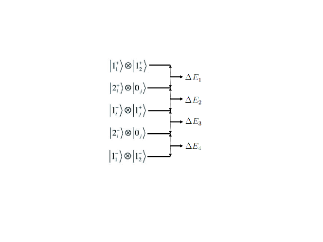
Figure 1: Energy levels for the two-cavity system in the absence of hopping (A=0), $\Delta E_{i}$ $(i=1,2,3,4)$ is the energy gap between the adjacent energy levels.

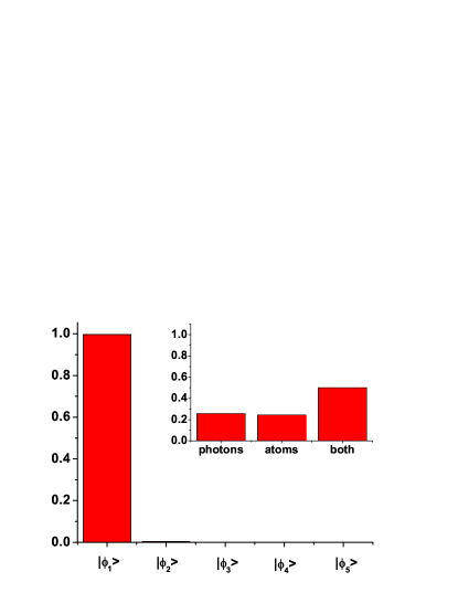
Figure 2: (Color online) Occupation probabilities of the ground state in the five subspaces. The inset shows the probability distribution of excitations among states with purely photonic, purely atomic, and mixed of them. The hopping strength between the two cavities is weak for $A=0.1g$, the detuning between the atom and the field is $\Delta=0$, and the atom-atom coupling strength is $J=0.1g$.

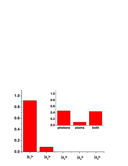
Figure 3: (Color online) Occupation probabilities of the ground state in the five subspaces. The inset shows the probability distribution of excitations among states with purely photonic, purely atomic, and mixed of them. The hopping strength between the two cavities is weak for $A=0.1g$, the detuning between atom and field is $\Delta=0$, and the atom-atom coupling strength is $J=g$.

III The nature of the ground state

In the weak cavity-cavity coupling limit, we can understand the nature of the ground state by considering the effects of parameters in the effective Hamiltonian in Eq.(4). In fact, the energy gap $\Delta E_{i}$ $(i=1,2,3,4)$ between the five subspaces not only dependents on the atom-field coupling strength $g$ and detuning $\Delta$, but also relies on the atom-atom coupling strength $J$, which is shown in Fig.1.

where

$$\Delta E_{1} = \sqrt{(\Delta+J)^{2}+8g^{2}}$$

$$- \frac{1}{2}[\sqrt{(\Delta+J)^{2}+16g^{2}}+(\Delta+J)],$$

$$\Delta E_{2} = \frac{1}{2}[(\Delta+J)+\sqrt{(\Delta+J)^{2}+16g^{2}}],$$

$$\Delta E_{3} = \frac{1}{2}[\sqrt{(\Delta+J)^{2}+16g^{2}}-(\Delta+J)],$$

$$\Delta E_{4} = \sqrt{(\Delta+J)^{2}+8g^{2}}$$ (8)

$$- \frac{1}{2}[\sqrt{(\Delta+J)^{2}+16g^{2}}-(\Delta+J)].$$

To illustrate the behavior of the ground state operating in the dipole-dipole interaction, we first pay our attention to the resonant condition $\Delta=0$, and three cases for $J\ll g$, $J\approx g$, and $J\gg g$ will be discussed in the following.

At $J\ll g$, there is a large energy gap between $|\phi_{1}\rangle$ and $|\phi_{2}\rangle$ due to the photon blockade effect, for which the presence of one photon in the cavity blocks the entering of the subsequent photons. On this condition, the ground state of the system is approximately $|1^{-}_{1}\rangle\otimes|1^{-}_{2}\rangle$, as shown in Fig.2. Moreover, $|1^{-}\rangle$ is nearly the maximal entanglement state of atom and field. For this state, only one excitation in each cavity with almost equal probabilities for atomic and field excitations. This can also be confirmed from the inset of Fig.2. Thus the ground state is a polaritonic insulatorlike state, which is analogous to the Mott insulator state in the Bose-Hubbard model.

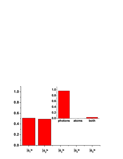
Figure 4: (Color online) (Occupation probabilities of the ground state in the five subspaces. The inset shows the probability distribution of excitations among states with purely photonic, purely atomic, and mixed of them. The hopping strength between the two cavities is weak for $A=0.1g$, the detuning between atom and field is $\Delta=0$, and the atom-atom coupling strength is $J=10g$.

Figure 5: The energy gap $\Delta E_{1}$ versus dipole coupling strength $J$ at $\Delta=0$. The hopping strength between the two cavities is weak for $A=0.1g$.

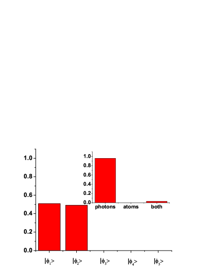
Figure 6: (Color online) Occupation probabilities of the ground state in the five subspaces. The inset shows the probability distribution of excitations among states with purely photonic, purely atomic, and mixed of them. For large positive atom-field detuning, the effects of the dipole coupling strength can be ignored. Here, we choose $A=0.1g$, $\Delta=10g$ and $J=g$.

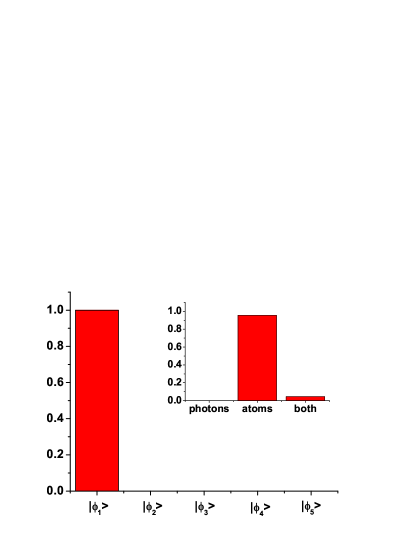
Figure 7: (Color online) Occupation probabilities of the ground state in the five subspaces. The inset shows the probability distribution of excitations among states with purely photonic, purely atomic, and mixed of them. For large negative atom-field detuning, two cases of weak and strong dipole coupling strength are shown. Here, we choose $A=0.1g$ and $\Delta=-10g$. Other parameter value is $J=0.1g$.

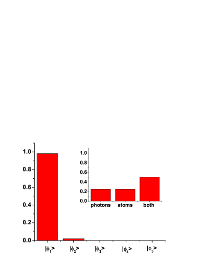
Figure 8: (Color online) Occupation probabilities of the ground state in the five subspaces. The inset shows the probability distribution of excitations among states with purely photonic, purely atomic, and mixed of them. For large negative atom-field detuning, two cases of weak and strong dipole coupling strength are shown. Here, we choose $A=0.1g$ and $\Delta=-10g$. Other parameter value is $J=10g$.

Compared to Fig.2, Figure 3 indicates a more different behavior for $J\approx g$. Besides $|\phi_{1}\rangle$, the subspace $|\phi_{2}\rangle$ is also occupied for the ground state of the system. From its inset, we find that both the atom and the field are excited, indicating a polaritonic superfluidlike state.

When $J\gg g$, the ground state occupies the subspaces $|\phi_{1}\rangle$ and $|\phi_{2}\rangle$ with almost same probabilities, as represented in Fig.4. However, only the photons are excited in this state. This is because, in this limit, $|n^{-}\rangle\approx-|gn\rangle$, so the ground state is a delocalized photon state in nature. The state of this form is a photonic superfluidlike state.

The results can be understood easily. Similar to the effect of detuning in Ref.Irish , at $\Delta=0$, the energy gap of $\Delta E_{1}$ is a monotonic decreasing function of $J$, see Fig.5. With the increase of $J$, the photon blockade effect is destroyed, leading to an increase of the occupied probability of $|\phi_{2}\rangle$. When $J\approx 10g$, $\Delta E_{1}$ is almost zero, so the subspaces $|\phi_{1}\rangle$ and $|\phi_{2}\rangle$ nearly degenerate. Oppositely, $\Delta E_{2}$ is a monotonic increasing function of $J$ with a large initial value. Thus, the subspace $|\phi_{3}\rangle$ can not be occupied.

Next, we discuss the case of large positive detuning. At $\Delta=0$, the nature of the ground state changes with different values of $J$. However, when $\Delta\gg g$, no matter what value of $J$, the energy gap of $\Delta E_{1}$ is always zero. While $\Delta E_{2}$ is a monotonic increasing function of $\Delta+J$. Even $J=0$, the energy gap $\Delta E_{2}$ is very large. Therefore, the ground state has equal occupation probabilities in the subspaces $|\phi_{1}\rangle$ and $|\phi_{2}\rangle$, but zero probability in other subspaces. More interestingly, in the large positive detuning limit, the superposition coefficients of the dressed states in Eq.(5) have particular values, $\sin\frac{\theta_{n}}{2}$$\approx 0$ and $\cos\frac{\theta_{n}}{2}$$\approx 1$. Then, $|n^{-}\rangle\approx-|g\rangle|n\rangle$. Consequently, not only the constitution of the ground state but also its nature is fixed. In Fig.6, the inset shows that the excitation is photonic rather than atomic. This is because the energy of the atoms is larger than that of the photons when $\Delta>0$. Analogous to the situation shown in Fig.4, the ground state indicates photonic superfluidlike nature.

At $\Delta<0$, the energy of atoms is smaller than that of photons. In the limit of $-\Delta\gg g,J$, we find $\Delta E_{1}\approx|\Delta|$, the ground state is approximate $|1^{-}_{1}\rangle\otimes|1^{-}_{2}\rangle$. In this condition, $\sin\frac{\theta_{n}}{2}$$\approx 1$ and $\cos\frac{\theta_{n}}{2}$$\approx 0$. Thus, $|1^{-}\rangle\approx|e\rangle|0\rangle$, The excitation is almost atomic rather than photonic, standing for an atomic insulatorlike state. The result is illustrated in Fig.7. However, when $J$ approaches to the value of $-\Delta$, the value of $|\Delta+J|$ decreases. That is, the energy difference between atom and photon is less and less. As a result, the photonic and atomic excitations coexist, as shown in Fig.8, corresponding to the polaritonic insulatorlike state.

IV Phase diagrams

The phase diagrams of these states can be distinguished using the corresponding “order parameters”. In superfluid states, the excitations in each cavity is uncertain, resulting in a nonzero variance of the total excitation number $\Delta N_{1}$. Oppositely, in the insulator state the number of excitations per cavity is constant and thus has zero variance. However, the insulator state may be either atomic or polaritonic and the superfluid state may be photonic or polaritonic in nature. To determine the allowed types of particles involved in the state, the atomic excitation number variance $\Delta N_{A1}$ should be taken as the “order parameter”. $\Delta N_{A1}=0$ is corresponding to the atomic insulator state or the photonic superfluid state, while $\Delta N_{A1}>0$ revealing the polaritonic nature. Only when $\Delta N_{1}\Delta N_{A1}>0$, it shows the polaritonic superfluid characteristic for the ground state of the system.

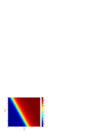
Figure 9: (Color online) For weak hopping strength $A=0.1g$, $\Delta N_{1}$ is plotted versus atom-field detuning $\Delta$ and dipole coupling strength $J$ in the ground state of the coupled two-site and two-excitation system.

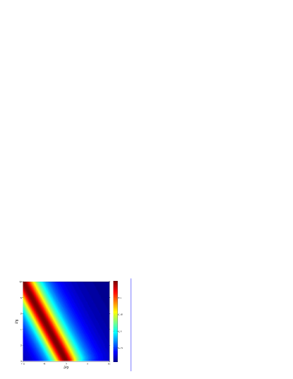
Figure 10: (Color online) For weak hopping strength $A=0.1g$, $\Delta N_{A1}$ is plotted versus atom-field detuning $\Delta$ and dipole coupling strength $J$ in the ground state of the coupled two-site and two-excitation system.

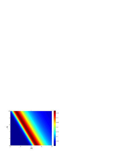
Figure 11: (Color online) For weak hopping strength $A=0.1g$, $\Delta N_{1}\cdot\Delta N_{A1}$ is plotted versus atom-field detuning $\Delta$ and dipole coupling strength $J$ in the ground state of the coupled two-site and two-excitation system.

To begin with, we should distinguish the insulator and superfluid areas in the phase diagram, which are determined by the total excitation number $\Delta N_{1}$. With Eq.(4), we can give out the expression of $\Delta N_{1}$ directly.

$$N_{1} = a^{\dagger}_{1}a_{1}+\sigma_{1}^{{\dagger}}\sigma_{1},$$

$$\Delta N_{1} = \langle N^{2}_{1}\rangle-\langle N_{1}\rangle^{2}.$$ (9)

In Fig.9, $\Delta N_{1}$ is plotted under a wide range values of the atom-cavity detunings $\Delta$ and the dipole-dipole interaction strength $J$. It is apparent that the phase diagram is divided into two sections. The insulator region is under the boundary where $\Delta<0$ while above the boundary is the superfluid region. There is also an area which is symmetric to the insulator area, where the $\Delta N_{1}$ with a maximum value 0.5, indicating a most evident superfluidity.

To find out the polaritonic area, we should introduce the second “order parameters” $\Delta N_{A1}$, where

$$N_{A1} = a^{\dagger}_{1}a_{1}+\sigma_{1}^{{\dagger}}\sigma_{1},$$

$$\Delta N_{A1} = \langle N^{2}_{A1}\rangle-\langle N_{A1}\rangle^{2}.$$ (10)

In Fig.10, we find that the polaritonic area approximately spreads at both sides of the line $J=-\Delta$. The more closer to the line the more obvious the polaritonic nature. In fact, when $J=-\Delta$, $\Delta E_{1}=(2\sqrt{2}-2)g$, it is the conditions for photon blockade effect obviously. Then the ground state only occupies the subspace $|\phi_{1}\rangle$, with $\sin\frac{\theta_{n}}{2}=\cos\frac{\theta_{n}}{2}=\frac{1}{2}$, standing for a maximal entanglement state of the atom and the field. So the ground state indicates polaritonic insulatorlike nature.

So far we may guess that on the bases of what are embodied in Fig.9 and Fig.10, there must be some overlapped areas in the two figures. In Fig.11, the product of $\Delta N_{1}$ and $\Delta N_{A1}$ is shown as a contour plot. We can clearly identify that there is an area not only in the superfluid region in Fig.9, but also in the polaritonic area in Fig.10, representing polaritonic superfluidlike characters.

Then it is obvious that the phase space in Fig.9 is divided into four sections, from left bottom to top right corner, in order of atomic insulatorlike region, polaritonic insulatorlike region, polaritonic superfluidlike region and photonic superfluidlike region.

V Conclusions

In summary, we have investigated the QPT of a system composed of two coupled cavities, each containing a pair of two-level atoms with dipole-dipole interaction. In the conditions of fixed cavity-cavity interaction and atom-cavity coupling strength, the nature of the ground state is dependent on the constituents of the dressed states in each cavity and the occupation probabilities of the ground state in the five subspaces. Moreover, both of them attribute to the dipole-dipole interaction strength between the localized atoms and the atom-field detuning in each cavity. By choosing three different order parameters, we found that the ground state of the system represented more richer behaviors than the Bose-Hubbard model. Four types of states are revealed, which divide the phase space into four regions. They are the atomic insulatorlike state, the polaritonic insulatorlike state, the polaritonic superfluidlike state and the photonic superfluidlike state. In the scope of parameter values we taken in this paper, the insulator or superfluid phases is determined by the combinative effect of $\Delta$ and $J$, that is the value of $\Delta+J$. Small negative values of it is in favour of polaritonic insulatorlike states while for small positive value of it embodies polaritonic superfluidlike state. The more larger negative value of $\Delta+J$, the more obvious of atomic insulatorlike nature, and oppositely it shows photonic superfluidlike nature.

- (1) M. Greiner, et al., Nature (London) 415, 39 (2002).
- (2) I. Bloch, J. Dalibard, and W. Zwerger, Rev. Mod. Phys. 80, 885 (2008).
- (3) D. Jaksch, C. Bruder, J. I. Cirac, C. W. Gardiner, and P. Zoller, Phys. Rev. Lett. 81, 3108 (1998).
- (4) A. Albus, F. Illuminati, and J. Eisert, Phys. Rev. A 68, 023606 (2003).
- (5) V. W. Scarola and S. Das Sarma, Phys. Rev. Lett. 95, 033003 (2005).
- (6) C. Maschler and H. Ritsch, Phys. Rev. Lett. 95, 260401 (2005).
- (7) I. B. Spielman, W. D. Phillips, and J. V. Porto, Phys. Rev. Lett. 98, 080404 (2007).
- (8) U. Schneider, et al., Science 322, 1520 (2008).
- (9) R. Jrdens, et al., Nature (London) 455, 204 (2008).
- (10) K. JiménezGarcía, et al., Phys. Rev. Lett. 105, 110401 (2010).
- (11) M. J. Hartmann, F. G. S. L. Brando, and M. B. Plenio, Nat. Phys. 2, 849 (2006).
- (12) A. D. Greentree, C. Tahan, J. H. Cole, and L. C. L. Hollenberg, Nat. Phys. 2, 856 (2006).
- (13) D. G. Angelakis, M. F. Santos, and S. Bose, Phys. Rev. A 76, 031805(R) (2007).
- (14) M. J. Hartmann, F. G. S. L. Brando, and M. B. Plenio, Laser Photon. Rev. 2, 527 (2008).
- (15) D. Rossini and R. Fazio, Phys. Rev. Lett. 99, 186401 (2007).
- (16) M. Aichhorn, M. Hohenadler, C. Tahan, and P. B. Littlewood, Phys. Rev. Lett. 100, 216401 (2008).
- (17) J. Cho, D. G. Angelakis, and S. Bose, Phys. Rev. Lett. 101, 246809 (2008).
- (18) I. Carusotto, et al., Phys. Rev. Lett. 103, 033601 (2009).
- (19) S. Schmidt and G. Blatter, Phys. Rev. Lett. 103, 086403 (2009).
- (20) J. Koch and K. L. Hur, Phys. Rev. A 80, 023811 (2009).
- (21) M. J. Hartmann, Phys. Rev. Lett. 104, 113601 (2010).
- (22) A. Tomadin, et al., Phys. Rev. A 81, 061801(R) (2010)
- (23) A. Tomadin and R. Fazio, J. Opt. Soc. Am. B 27, A130(2010).
- (24) F. Ciccarello, Phys. Rev. A 83, 043802 (2011).
- (25) J. M. Raimond, M. Brune and S. Haroche, Rev. Mod. Phys. 73, 565 (2001).
- (26) K. M. Birnbaum, et al., Nature(London) 436, 87 (2005).
- (27) J. P. Reithmaier et al., Nature(London) 432, 197 (2004)
- (28) K. Hennessy, et al., Nature(London) 445, 896 (2007).
- (29) E. K. Irish, C. D. Ogden, and M. S. Kim, Phys. Rev. A 77, 033801 (2008).
- (30) C. D. Ogden, E. K. Irish, and M. S. Kim, Phys. Rev. A 78, 063805 (2008).
- (31) Z. B. Yang, H. Z. Wu, W. J. Su, and S. B. Zheng, Phys. Rev. A 80, 012305 (2009).
- (32) E. K. Irish, Phys. Rev. A 80, 043825 (2009).
- (33) K. Zhang and Z. Y. Li, Phys. Rev. A 81, 033843 (2010).
- (34) S. Ferretti and L. C. Andreani, Phys. Rev. A 82, 013841 (2010).
- (35) S. Schmidt, D. Gerace, A. A. Houck, G. Blatter, and H. E. Treci, Phys. Rev. B 82, 100507(R) (2010).
- (36) X. Y. Guo and Z. Z. Ren, Phys. Rev. A 83, 013809 (2011).
- (37) M. Knap, E. Arrigoni, and W. von der Linden, J. H. Cole, Phys. Rev. A 83, 023821 (2011).
- (38) M. Scheibner et al., Nat. Phys. 3, 106 (2007).
- (39) D. Schneble et al., Science 300, 475 (2003).
- (40) S. Nicolosi, et al., Phys. Rev. A 70, 022511 (2004).
- (41) H. Wang, S. Q. Liu, and J. Z. He, Phys. Rev. E 79, 041113 (2009).
- (42) P. B. Li, Y. Gu, Q. H. Gong, and G. C. Guo, Phys. Rev. A 79, 042339 (2009).