Period- and Mirror-maps for the Quartic K3

Abstract.

We study in detail mirror symmetry for the quartic K3 surface in ${\mathbb{P}}^{3}$ and the mirror family obtained by the orbifold construction. As explained by Aspinwall and Morrison [AM97], mirror symmetry for K3 surfaces can be entirely described in terms of Hodge structures.
- We give an explicit computation of the Hodge structures and period maps for these families of K3 surfaces.
- We identify a mirror map, i.e. an isomorphism between the complex and symplectic deformation parameters and explicit isomorphisms between the Hodge structures at these points.
- We show compatibility of our mirror map with the one defined by Morrison [Mor92] near the point of maximal unipotent monodromy.
Our results rely on earlier work by Narumiyah–Shiga [NS01], Dolgachev [Dol96] and Nagura–Sugiyama [NS95].

1. Introduction

Let $(X,I,\omega_{X})$ be a Calabi–Yau manifold with complex structure $I$ and chosen Kähler form $\omega_{X}$. The philosophy of mirror symmetry says that certain invariants of the complex manifold $(X,I)$ should be encoded by the symplectic structure $\omega_{Y}$ of a mirror Calabi–Yau $(Y,J,\omega_{Y})$ and vice versa.

Following Aspinwall and Morrison [AM97] (see also [Huy04] and [Huy05]), mirror symmetry for K3 surfaces can be described in terms of Hodge structures. To a K3 surface $(X,I,\omega_{X})$ with chosen Kähler form $\omega_{X}$ we associate two Hodge structures $H_{A},H_{B}$ on the lattice $H^{*}(X,{\mathbb{Z}})$. The essential fact is, that $H_{A}$ only depends on the symplectic form $\omega_{X}$ and $H_{B}$ only on the complex structure $I$. Now $(X,I)$ is said to be mirror dual to $(Y,\omega_{Y})$ in the Hodge theoretic sense if there exists a Hodge isometry

$$H_{B}(X,{\mathbb{Z}})\cong H_{A}(Y,{\mathbb{Z}}).$$

This definition can be seen as a refinement of Dolgachev’s [Dol96] notion of mirror symmetry for families of lattice polarized K3 surfaces (cf. section 2.5). There are many examples of mirror dual families of lattice polarized K3 surfaces, e.g. [Bel02], [Roh04], [Dol96]. On the other hand, the author is not aware of an explicit example of mirror symmetry in the Hodge theoretic sense in the literature.

We study the following families of K3 surfaces.

• Let $Y\subset{\mathbb{P}}^{3}$ be a smooth quartic in ${\mathbb{P}}^{3}$ viewed as a symplectic manifold with the symplectic structure given by the restriction of the Fubini–Study Kähler form $\omega_{FS}$. We introduce a scaling parameter $p\in{\mathbb{H}}$ to get a family of (complexified) symplectic manifolds $Y_{p}=(Y,\omega_{p}),\;\omega_{p}=p/i\cdot\omega_{FS}$ parametrized by the upper half plane.

• Let $X_{t}$ be the Dwork family of K3 surfaces, which is constructed from the Fermat pencil

  $$F_{t}:=\{X_{0}^{4}+X_{1}^{4}+X_{2}^{4}+X_{3}^{4}-4tX_{0}X_{1}X_{2}X_{3}=0\}\subset{\mathbb{P}}^{3}$$

  by taking the quotient with respect to a finite group and minimal resolution of singularities.

This is the two-dimensional analog to the quintic threefold and its mirror studied by Candelas et al. [COGP91].

Theorem 1.1 (Theorem 5.1, Theorem 4.29, Theorem 4.37).

The K3 surfaces $X_{t}$ and $Y_{p}$ are mirror dual in the Hodge theoretic sense if $t$ and $p$ are related by

$$exp(2\pi ip) =w+104\,{w}^{2}+15188\,{w}^{3}+2585184\,{w}^{4}+480222434\,{w}^{5}+\dots$$

where $w:=1/(4t)^{4}$. A closed expression as ratio of hypergeometric functions is given in section 4.7.

The multi-valued map $\psi:z\mapsto p(z),z=1/t^{4}$ determined by this equation is a Schwarz triangle function which maps the upper half plane to the hyperbolic triangle with vertices $(\infty,\frac{i}{\sqrt{2}},\frac{1+i}{2})$ and interior angles $(0,\pi/2,\pi/4)$, as pictured in Figure 1.

The proof relies heavily on earlier work by Narumiyah and Shiga [NS01], Dolgachev [Dol96] and Nagua and Sugiyama [NS95]. We proceed in three main steps: First, we use a theorem of Narumiyah and Shiga which provides us with the required cycles and a description of the topological monodromy of the family. Then we consider the Picard–Fuchs differential equation which is satisfied by the period integrals. We derive a criterion for a set of solutions to be the coefficients of the period map. In a third step we construct solutions to this differential equation which match this criterion. Here we use the work of Nagura and Sugiyama. The relation to Schwarz triangle function appears also in [NS01, Thm. 6.1].

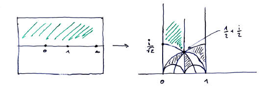
Figure 1. Mapping behavior of the mirror map $\psi$ in coordinates $z=1/t^{4}$ and $p$.

The function in Theorem 1.1 was also considered by Lian and Yau [LY96] (see Remark 5.2). There it was noted that the inverse function $z(p)$ is a modular form with integral Fourier expansion which is related to the Thompson series for the Griess–Fischer (“monster”) group. See also the exposition by Verrill and Yui in [VY00].

Our motivation for studying this specific family stems from a theorem of Seidel. Recall that the homological mirror symmetry conjecture due to Kontsevich [Kon95] states that if $(X,I)$ is mirror dual to $(Y,\omega_{Y})$ then then there is an exact equivalence of triangulated categories

$${\mathcal{D}}^{b}(Coh(X,I))\cong{\mathcal{D}}^{\pi}(Fuk(Y,\omega_{Y})).$$

There are only a few cases where such an equivalence is known to hold. One example was provided by Seidel. He proves homological mirror symmetry for the pair of K3 surfaces considered above.

Theorem (Seidel [Sei03]).

If the family $X_{t}$ is viewed as a K3 surface $X$ over the Novikov field $\Lambda_{{\mathbb{Q}}}(1/t)$, which is the algebraic closure of the field of formal Laurent series ${\mathbb{C}}((1/t))$, then there is an isomorphism $\psi:\Lambda_{{\mathbb{Q}}}(1/t)\cong\Lambda_{{\mathbb{Q}}}(q)$ and an equivalence of triangulated $\Lambda_{{\mathbb{Q}}}(q)$-linear categories

$$\psi_{*}{\mathcal{D}}^{b}(Coh(X))\cong{\mathcal{D}}^{\pi}(Fuk(Y)).$$

Unfortunately, the isomorphism $\psi$ has not yet been determined explicitly. Geometrically it describes the dependence of the symplectic volume $p$ of the quartic from the deformation parameter $t$ of the complex structure on $X$. Thus our mirror map $\psi$ in Theorem 1.1 provides a conjectural candidate for this isomorphism.

On the way to proving Theorem 1.1 we also give an explicit calculation of the classical period map for the Dwork family. Consider a non-zero holomorphic two-form $\Omega\in H^{2,0}(X)$ and a basis of two-dimensional cycles $\Gamma_{i}\in H_{2}(X,{\mathbb{Z}})\cong{\mathbb{Z}}^{22}$. By the global Torelli theorem, the complex structure on $X$ is determined by the period integrals $(\int_{\Gamma_{1}}\Omega,\dots,\int_{\Gamma_{22}}\Omega)$ and the intersection numbers $\Gamma_{i}.\Gamma_{j}$.

Theorem 1.2 (Theorem 4.29, Remark 4.32).

For $t\in{\mathbb{C}}$ near $t_{0}=i/\sqrt{2}$, there are explicit bases $\Gamma_{i}(t)\in H_{2}(X_{t},{\mathbb{Z}}),i=1,\dots,22$ and holomorphic two forms $\Omega_{t}$ on the Dwork family $X_{t}$ such that the period integrals are given by

$$(\int_{\Gamma_{1}(t)}\Omega_{t},\dots,\int_{\Gamma_{22}(t)}\Omega_{t})=(4p(t),2p(t)^{2},-1,p(t),0,\dots,0),$$

where $p(t)=\psi(1/t^{4})$ is the function introduced in Theorem 1.1.

Acknowledgments. This work is part of my PhD thesis written under the supervision of Prof. Daniel Huybrechts to whom I owe much gratitude for his constant support and encouragement. I thank Duco van Straten for explaining to me much about hypergeometric functions and Picard–Fuchs equations.

2. Mirror symmetry for K3 surfaces

In this section we summarize Aspinwall and Morrison’s description [AM97] of mirror symmetry for K3 surfaces in terms of Hodge structures. Their constructions have been generalized to higher dimensional hyperkähler manifolds by Huybrechts in [Huy04] and [Huy05].

2.1. The classical Hodge structure of a complex K3 surface

Recall from [BBD85] that a K3 surface is a two-dimensional connected complex manifold $X$ with trivial canonical bundle $\Omega^{2}_{X}\cong{\mathcal{O}}_{X}$ and $H^{1}(X,{\mathcal{O}}_{X})=0$.

The second cohomology $H^{2}(X,{\mathbb{Z}})$ endowed with the cup-product pairing $(a.b)=\int a\cup b$ is an even, unimodular lattice of rank 22 isomorphic to the K3 lattice $\Lambda:=2E_{8}(-1)\oplus 3U$. The group $H^{2,0}(X)=H^{0}(X,\Omega^{2}_{X})$ is spanned by a the class of a holomorphic two form $\Omega$ which is nowhere vanishing. This class satisfies the properties

$$(\Omega.\Omega)=0\,\qquad(\Omega.\bar{\Omega})>0.$$

Remark 2.1.

The Hodge structure on $H^{2}(X,{\mathbb{Z}})$ is completely determined by the subspace $H^{2,0}(X)\subset H^{2}(X,{\mathbb{C}})$. Indeed, we have

$$H^{0,2}(X)=\overline{H^{2,0}(X)}\quad\text{and}\quad H^{1,1}(X)=(H^{2,0}(X)\oplus H^{0,2}(X))^{\perp}.$$

The global Torelli theorem states that a K3 surface is determined up to isomorphy, by it’s Hodge structure.

Theorem 2.2 (Piatetski-Shapiro–Shafarevich, Burns–Rapoport).

Two K3 surfaces $X,X^{\prime}$ are isomorphic if and only if there is a Hodge isometry $H^{2}(X,{\mathbb{Z}})\cong H^{2}(X^{\prime},{\mathbb{Z}})$.

2.2. CFT-Hodge structures of complex K3 surfaces

There is another weight-two Hodge structure associated to a K3 surface, which plays an important role for mirror symmetry.

Define the Mukai pairing on the total cohomology $H^{*}(X,{\mathbb{Z}})$ by

(1) $$((a_{0},a_{2},a_{4}).(b_{0},b_{2},b_{4})):=\int a_{2}\cup b_{2}-a_{0}\cup b_{4}-a_{4}\cup b_{2}.$$

We denote this lattice by $\tilde{H}(X,{\mathbb{Z}})$. It is an even, unimodular lattice of rank $24$ and signature $(4,20)$ isomorphic to the enlarged K3 lattice $\tilde{\Lambda}:=\Lambda\oplus U$.

We define a weight-two Hodge structure on $\tilde{H}(X,{\mathbb{Z}})$ by setting $H_{B}^{2,0}(X)=H^{2,0}(X)$ and using the construction in Remark 2.1. Note that

$$H_{B}^{1,1}(X)=H^{0}(X,{\mathbb{C}})\oplus H^{1,1}(X)\oplus H^{4}(X,{\mathbb{C}}).$$

We call $H_{B}(X,{\mathbb{Z}})=(\tilde{H}(X,{\mathbb{Z}}),(\,.\,),H_{B}^{p,q}(X))$ the B-model Hodge structure of $X$. The name is motivated by the statement in [AM97], that the “B-model conformal field theory” associated to $X$ is uniquely determined by $H_{B}(X,{\mathbb{Z}})$.

One very important occurrence of this Hodge structure is the following theorem.

Theorem 2.3 (Derived global Torelli; Orlov [Orl97]).

Two projective K3 surfaces $X,X^{\prime}$ have equivalent derived categories ${\mathcal{D}}^{b}(X)\cong{\mathcal{D}}^{b}(X^{\prime})$ if and only if there exists a Hodge isometry $H_{B}(X,{\mathbb{Z}})\cong H_{B}(X^{\prime},{\mathbb{Z}})$.

2.3. CFT-Hodge structures of symplectic K3 surfaces

Every Kähler form $\omega$ on a K3 surface $X$ defines a symplectic structure on the underlying differentiable manifold. In this section we will associate a Hodge structure to this symplectic manifold. Moreover, we shall allow twists by a so called B-field $\beta\in H^{2}(X,{\mathbb{R}})$ to get a complexified version.

Given $\omega$ and $\beta$ we define the following class of mixed, even degree

(2) $$\mho=\exp(i\omega+\beta)=(1,i\omega+\beta,(i\omega+\beta)^{2}/2)\in\tilde{H}(X,{\mathbb{C}}).$$

This class enjoys formally the same properties as $\Omega\in H^{2,0}(X)$ above:

$$(\mho.\mho)=0,\quad(\mho.\overline{\mho})>0$$

with respect to the Mukai-pairing. Hence, we can define a Hodge structure $H_{A}(X,{\mathbb{Z}})$ on $\tilde{H}(X,{\mathbb{Z}})$ by demanding $H_{A}^{2,0}(X):={\mathbb{C}}\,\mho$ via Remark 2.1.

We call $H_{A}(X,{\mathbb{Z}})$ the A-model Hodge structure of $(X,\omega,\beta)$. Again, the name is motivated by the statement in [AM97], that the “A-model conformal field theory” associated to $(X,\omega,\beta)$ is uniquely determined by $H_{A}(X,{\mathbb{Z}})$.

2.4. Mirror symmetries

Two Calabi–Yau manifolds $X,Y$ form a mirror pair if the B-model conformal field theory associated to $X$ is isomorphic to the A-model conformal field theory associated to $Y$. This motivates the following definition.

Definition 2.4.

A complex K3 surface $X$ with holomorphic two-form $\Omega$ and a symplectic K3 surface $Y$ with complexified Kähler form $\mho=\exp(i\omega+\beta)$ form a mirror pair if there exists a Hodge isometry

$$H_{B}(X,{\mathbb{Z}})\cong H_{A}(Y,{\mathbb{Z}}).$$

Thus a naive translation of Kontsevich’s homological mirror conjecture reads as follows.

Conjecture 2.5.

Let $X$ be a K3 surface with holomorphic two-form $\Omega$ and $Y$ a K3 surface with Kähler form $\omega$. Then there is an exact equivalence of triangulated categories

$${\mathcal{D}}^{b}(Coh(X))\cong{\mathcal{D}}^{\pi}(Fuk(Y))$$

if and only if there is a Hodge isometry $H_{B}(X,{\mathbb{Z}})\cong H_{A}(Y,{\mathbb{Z}}).$

Note that this is perfectly consistent with Orlov’s derived global Torelli theorem.

2.5. Relation to mirror symmetry for lattice polarized K3 surfaces

In this subsection we compare the Hodge theoretic notion of mirror symmetry to Dolgachev’s version for families of lattice polarized K3 surfaces [Dol96]. See also [Huy04, Sec. 7.1] and [Roh04, Sec. 2].

Let $M\subset\Lambda$ be a primitive sublattice. A $M$-polarized K3 surface is a K3 surface $X$ together with a primitive embedding $i:M\rightarrow Pic(X)$. We call $(X,i)$ pseudo-ample polarized if $i(M)$ contains a numerically effective class of positive self intersection.

Assume that $M$ has the property, that for any two primitive embeddings $i_{1},i_{2}:M\rightarrow\Lambda$ there is an isometry $g\in O(\Lambda)$ such that $i_{2}=g\circ i_{1}$. Then, there is a coarse moduli space $K_{M}$ of pseudo-ample $M$-polarized K3 surfaces.

Fix a splitting $M^{\perp}=U\oplus\hat{M}$. The above condition ensures, that the isomorphism class of $\hat{M}$ is independent of this choice.

Definition 2.6.

The mirror moduli space of $K_{M}$ is $K_{\hat{M}}$.

Symplectic structures on a K3 surface $Y$ in $K_{\hat{M}}$ correspond to points of the mirror moduli space $K_{M}$ in the following way:

Let $(Y,j)\in K_{\hat{M}}$ be an $\hat{M}$-polarized K3 surface with a marking, i.e. an isometry $n:H^{2}(Y,{\mathbb{Z}})\rightarrow\Lambda$, such that $j=n^{-1}|_{\hat{M}}$. Let $\omega+i\beta\in H^{2}(Y,{\mathbb{C}})$ be a complexified symplectic structure on $Y$, which is compatible with the $\hat{M}$-polarization, i.e. $\omega+i\beta\in j(\hat{M})_{{\mathbb{C}}}$. Denote by $\mho=exp(i\omega\oplus\beta)$ be the associated period vector.

The chosen splitting $M^{\perp}=\hat{M}\oplus U$ determines an isometry of $\xi\in O(\tilde{H}(Y,{\mathbb{Z}}))$ which interchanges the hyperbolic plane $n(U)$ with $H^{0}(Y,{\mathbb{Z}})\oplus H^{4}(Y,{\mathbb{Z}})$ and leaves the orthogonal complement fixed.

By construction the vector $\Omega:=\xi(\mho)$ lies in $n(U)_{{\mathbb{C}}}\oplus\hat{M}_{{\mathbb{C}}}\subset H^{2}(Y,{\mathbb{C}})$. Note that $(\Omega.\Omega)=0$ and $(\Omega.\bar{\Omega})>0$. Hence, by the surjectivity of the period map [BBD85, Exp. X], there exists a complex K3 surface $X$ and a isometry $g:H^{2}(Y,{\mathbb{Z}})\rightarrow H^{2}(X,{\mathbb{Z}})$ that maps $\Omega$ into $H^{2,0}(X)$. Extend $g$ to an isometry of Mukai lattices $\tilde{g}$, then

$$\tilde{g}\circ\xi:H_{A}(Y,{\mathbb{Z}})\longrightarrow H_{B}(X,{\mathbb{Z}})$$

is an Hodge isometry. Moreover, the marking of $Y$ induces an $M$-polarization of $X$ via

$$i:M\subset\Lambda\overset{n}{\longrightarrow}H^{2}(Y,{\mathbb{Z}})\overset{g}{\longrightarrow}H^{2}(X,{\mathbb{Z}}).$$

This means $(X,i)$ lies in the mirror moduli space $K_{M}$.

Conversely, if $\Omega\in H^{2.0}(X)$ is the period vector of a marked $M$-polarized K3 surface, then $\mho=\xi(\Omega)$ lies in $H^{0}(X,{\mathbb{C}})\oplus\hat{M}_{{\mathbb{C}}}\oplus H^{4}(X,{\mathbb{C}})$. Hence $\mho$ is of the form

$$\mho=a\,exp(i\omega+\beta)$$

for some $\omega,\beta\in M_{{\mathbb{R}}}$, $a\in{\mathbb{C}}^{*}$. Indeed, write $\mho=(a,c,b)$ with respect to the above decomposition, then $-2ab+c^{2}=0$ since $\mho^{2}=0$. Therefore $a\neq 0$ and we can set $i\omega+\beta:=c/a\in M_{{\mathbb{C}}}$.

Note that $\omega^{2}>0$ since $\mho.\bar{\mho}>0$. Now assume, that $\omega$ is represented by a symplectic form, then $i\omega+\beta$ defines a complexified symplectic structure on $Y=X$ such that

$$H_{B}(X,{\mathbb{Z}})\cong H_{A}(Y,{\mathbb{Z}}).$$

2.6. Period domains

In order to compare Hodge structures on different manifolds, it is convenient to introduce the period domains classifying Hodge structures.

Let $(L,(\,.\,))$ be a lattice. The period domain associated to $L$ is the complex manifold

$$\mathscr{D}(L):=\left\{\,[\Omega]\in{\mathbb{P}}(L\otimes{\mathbb{C}})\;|\;(\Omega.\Omega)=0,\;(\Omega.\bar{\Omega})>0\,\right\}.$$

The orthogonal group $O(L,(\,.\,))$ acts on $\mathscr{D}(L)$ from the left.

The period domain carries a tautological variation of Hodge structures on the constant local system $L$. Indeed, the holomorphic vector bundle $L\otimes{\mathcal{O}}_{\mathscr{D}(L)}$ has a tautological sub-vector bundle ${\mathcal{F}}^{2}$ with fiber ${\mathbb{C}}\,\Omega\subset L\otimes{\mathbb{C}}$ over a point $[\Omega]\in\mathscr{D}(L)$. The Hodge filtration is determined by ${\mathcal{F}}^{2}$ via

(3) $${\mathcal{F}}^{2}\subset{\mathcal{F}}^{1}:=({\mathcal{F}}^{2})^{\perp}\subset L\otimes{\mathcal{O}}_{\mathscr{D}(L)}.$$

2.7. Periods of marked complex K3 surfaces

Let $\pi:X\rightarrow B$ be a smooth family of K3 surfaces. We have a local system

$$\mathcal{H}_{\mathbb{Z}}=\mathrm{\mathbb{R}}^{2}\pi_{*}\underline{{\mathbb{Z}}}_{X}$$

on $B$ with stalks isomorphic to the cohomology $H^{2}(X_{t},{\mathbb{Z}})$ of the fiber $X_{t}=\pi^{-1}(\{t\})$. It carries a quadratic form $(\,.\,):\mathcal{H}_{\mathbb{Z}}\otimes\mathcal{H}_{\mathbb{Z}}\rightarrow\mathcal{H}_{\mathbb{Z}}$ and a holomorphic filtration

$${\mathcal{F}}^{2}=\pi_{*}\Omega^{2}_{X/B}\subset{\mathcal{F}}^{1}:=({\mathcal{F}}^{2})^{\perp}\subset\mathcal{H}:=\mathcal{H}_{\mathbb{Z}}\otimes{\mathcal{O}}_{B}$$

restricting fiber wise to the cup product pairing and the Hodge filtration on $H^{2}(X_{t},{\mathbb{C}})$, respectively.

Suppose now, that the local system $\mathcal{H}_{\mathbb{Z}}$ is trivial, and we have chosen a marking, i.e. an isometric trivialization $m:\mathcal{H}_{\mathbb{Z}}\rightarrow\Lambda\otimes\underline{{\mathbb{Z}}}_{B}.$ We can transfer the Hodge filtration on $\mathcal{H}_{\mathbb{Z}}$ to the constant system $\Lambda$ via $m$ and get a unique map to the period domain

$$\mathscr{P}({\mathcal{F}}^{*},m):B\longrightarrow\mathscr{D}(\Lambda)$$

with the property that the pull-back of the tautological variation of Hodge structures agrees with $m({\mathcal{F}}^{*})$ as Hodge structures on $\Lambda\otimes\underline{{\mathbb{Z}}}_{B}$. If $\Omega$ is a local section of ${\mathcal{F}}^{2}$, then the period map is explicitly given by

$$\mathscr{P}({\mathcal{F}}^{*},m)(t)=[m(\Omega(t))]\in\mathscr{D}(\Lambda)$$

for $t\in B$.

2.8. CFT-Periods of marked complex K3 surfaces

In the same way, we define the periods of the enlarged Hodge structures. We endow the local system

$$\tilde{\mathcal{H}}_{\mathbb{Z}}:=\mathrm{\mathbb{R}}^{*}\pi_{*}\underline{{\mathbb{Z}}}_{X}=\mathrm{\mathbb{R}}^{0}\pi_{*}\underline{{\mathbb{Z}}}_{X}\oplus\mathrm{\mathbb{R}}^{2}\pi_{*}\underline{{\mathbb{Z}}}_{X}\oplus\mathrm{\mathbb{R}}^{4}\pi_{*}\underline{{\mathbb{Z}}}_{X}$$

with the Mukai pairing defined by the same formula (1) as above. The associated holomorphic vector bundle $\tilde{\mathcal{H}}=\tilde{\mathcal{H}}_{\mathbb{Z}}\otimes{\mathcal{O}}_{B}$ carries the B-model Hodge filtration

$${\mathcal{F}}_{B}^{2}:=\pi_{*}\Omega^{2}_{X/B}\subset{\mathcal{F}}_{B}^{1}:=({\mathcal{F}}_{B}^{2})^{\perp}\subset\tilde{\mathcal{H}}.$$

For every marking $\tilde{m}:\tilde{\mathcal{H}}_{\mathbb{Z}}\rightarrow\tilde{\Lambda}\otimes\underline{{\mathbb{Z}}}_{B}$ of this enlarged local system, we get an associated B-model period map

$$\mathscr{P}_{B}({\mathcal{F}}^{*}_{B},\tilde{m}):B\longrightarrow\mathscr{D}(\tilde{\Lambda}).$$

Remark 2.7.

A marking $m$ of $\mathcal{H}_{\mathbb{Z}}$ determines a marking of $\tilde{\mathcal{H}}_{\mathbb{Z}}$ by the following convention. There are canonical trivializing sections $1\in\mathrm{\mathbb{R}}^{0}\pi_{*}\underline{{\mathbb{Z}}}_{X}$ and $or\in\mathrm{\mathbb{R}}^{4}\pi_{*}\underline{{\mathbb{Z}}}_{X}$, satisfying $(1.or)=-1$ with respect to the Mukai pairing. Let $e,f$ be the standard basis of $U$ with intersections $(e.f)=1,(e.e)=(f.f)=0$. Then the map

$$m_{0}:\mathrm{\mathbb{R}}^{0}\pi_{*}\underline{{\mathbb{Z}}}_{X}\oplus\mathrm{\mathbb{R}}^{4}\pi_{*}\underline{{\mathbb{Z}}}_{X}\longrightarrow U\otimes\underline{{\mathbb{Z}}}_{B},\quad 1\mapsto e,\;or\mapsto-f$$

is an orthogonal isomorphism of local systems and the map

$$\tilde{m}:=m\oplus m_{0}:\tilde{\mathcal{H}}_{\mathbb{Z}}=\mathcal{H}_{\mathbb{Z}}\oplus(\mathrm{\mathbb{R}}^{0}\pi_{*}\underline{{\mathbb{Z}}}_{X}\oplus\mathrm{\mathbb{R}}^{4}\pi_{*}\underline{{\mathbb{Z}}}_{X})\longrightarrow(\Lambda\oplus U)\otimes\underline{{\mathbb{Z}}}_{B}=\tilde{\Lambda}\otimes\underline{{\mathbb{Z}}}_{B}.$$

defines a marking of $\tilde{\mathcal{H}}_{\mathbb{Z}}$.

2.9. CFT-Periods of marked symplectic K3 surfaces

Let $\pi:X\rightarrow B$ be a family of K3 surfaces, and $\omega\in H^{0}(B,\pi_{*}{\mathcal{A}}^{2}_{X/B})$ a $d_{X/B}$-closed two-form, that restricts to a Kähler form on each fiber $X_{t}$. The form $\omega$ determines a global section of

$$\mathcal{H}_{\infty}=(\mathrm{\mathbb{R}}^{2}\pi_{*}\underline{{\mathbb{Z}}}_{X})\otimes\mathscr{C}_{B}^{\infty}({\mathbb{C}})=\mathrm{\mathbb{R}}^{2}\pi_{*}({\mathcal{A}}^{*}_{X/B})={\mathcal{H}}^{2}(\pi_{*}{\mathcal{A}}^{*}_{X/B}).$$

Analogously, a closed form $\beta\in H^{0}(B,\pi_{*}{\mathcal{A}}^{2}_{X/B})$ gives a section $\beta\in H^{0}(B,\mathcal{H}_{\infty})$. Given $\omega$ and $\beta$ we define a section

$$\mho=\exp(i\omega+\beta)\in H^{0}(B,\tilde{\mathcal{H}}_{\infty}),\quad\tilde{\mathcal{H}}_{\infty}=\mathrm{\mathbb{R}}^{*}\pi_{*}{\mathbb{Z}}\otimes\mathscr{C}_{B}^{\infty}({\mathbb{C}})$$

by the same formula (2) used in the point-wise definition of $\mho$. We set the A-model Hodge filtration to be the sequence of $\mathscr{C}^{\infty}$-vector bundles

$${\mathcal{F}}^{2}_{A}:=\mathscr{C}_{B}^{\infty}({\mathbb{C}})\,\mho\subset{\mathcal{F}}^{1}_{A}:=({\mathcal{F}}^{2}_{A})^{\perp}\subset\tilde{\mathcal{H}}_{\infty}.$$

In the same way as above, every marking $\tilde{m}:\tilde{\mathcal{H}}_{\mathbb{Z}}\rightarrow\tilde{\Lambda}\otimes\underline{{\mathbb{Z}}}_{B}$ determines an A-model period map

$$\mathscr{P}_{A}({\mathcal{F}}_{A}^{*},\tilde{m}):B\longrightarrow\mathscr{D}(\tilde{\Lambda})$$

which is a morphism of $\mathscr{C}^{\infty}$-manifolds.

Example 2.8.

Given $d_{X}$-closed two-forms $\omega,\beta\in{\mathcal{A}}^{2}_{X}$ on $X$, we get $d_{X/B}$-closed relative two-forms via the canonical projection ${\mathcal{A}}^{*}_{X}\rightarrow{\mathcal{A}}^{*}_{X/B}$. In this case, the map $B\ni t\mapsto\exp(i\omega(t)+\beta(t))\in\tilde{H}(X_{t},{\mathbb{C}})$ factors through the pull-back

$$i^{*}:H^{*}(X,{\mathbb{C}})\longrightarrow H^{*}(X_{t},{\mathbb{C}})$$

along the inclusion $i:X_{t}\rightarrow X$. As this map is already defined on $H^{2}(\_,{\mathbb{Z}})$ the associated period map is constant.

We can extend this example a bit further. Let $\omega$ be a constant Kähler form as above and $f:B\rightarrow{\mathbb{H}}$ a holomorphic function to the upper half-plane. The form $f\omega=iIm(f)\omega+Re(f)\omega$ is $d_{X/B}$-closed and satisfies $(\exp(f\omega).\overline{\exp(f\omega)})>0$. Hence we get a period map

$$\mathscr{P}_{A}({\mathcal{F}}_{A}^{*},\tilde{m})(t)=[\tilde{m}(\exp(f(t)\omega))]\in\mathscr{D}(\tilde{\Lambda})$$

for $t\in B$, which is easily seen to be holomorphic.

2.10. Mirror symmetry for families

Let $\pi:X\rightarrow B$ be a family of complex K3 surfaces with marking and $\rho:Y\rightarrow C$ a family of K3 surfaces with marking and chosen relative complexified Kähler form $i\omega+\beta$.

Definition 2.9.

A mirror symmetry between $X$ and $Y$ consists of an orthogonal transformation $g\in O(\tilde{\Lambda})$ called global mirror map and an étale, surjective morphism $\psi:C\rightarrow B$ called geometric mirror map such that the following diagram is commutative.

In particular for every point $s\in C$ we have a mirror pair

$$H_{A}(Y_{s},{\mathbb{Z}})\cong H_{B}(X_{\psi(s)},{\mathbb{Z}}).$$

Remark 2.10.

A typical global mirror map will exchange the hyperbolic plane $H^{0}(X_{s},{\mathbb{Z}})\oplus H^{4}(X_{s},{\mathbb{Z}})$ with a hyperbolic plane inside $H^{2}(X_{s},{\mathbb{Z}})$ as in subsection 2.5. We will see, that this happens in our case, too. Examples for other mirror maps can be found in [Huy04, Sec. 6.4].

Note that, if the markings of $X$ and $Y$ are both induced by a marking of the second cohomology local system as in Remark 2.7 then $g$ can never be the identity. Indeed, we always have

$$H^{2,0}_{B}(X_{s})\perp(H^{0}(X_{s},{\mathbb{Z}})\oplus H^{4}(X_{s},{\mathbb{Z}}))$$

but never $H^{2,0}_{A}(Y_{t})\perp(H^{0}(Y_{t},{\mathbb{Z}})\oplus H^{4}(Y_{t},{\mathbb{Z}}))$ since $(\exp(i\omega+\beta).or)=-1.$

3. Period map for the quartic

Since the calculation of the period map for the symplectic quartic is much easier than for the Dwork family, we begin with this construction.

A smooth quartic in $Y\subset{\mathbb{P}}^{3}$ inherits a symplectic structure from ${\mathbb{P}}^{3}$ by restricting the Fubini–Study Kähler form $\omega_{FS}$. A classical result of Moser [Mos65] shows that all quartics are symplectomorphic.

Proposition 3.1.

For all primitive $h\in\Lambda$ with $\langle h,h\rangle=4$ there exists a marking $m:H^{2}(Y,{\mathbb{Z}})\rightarrow\Lambda$ such that $m([\omega])=h$.

Proof.

Recall that $[\omega]=[\omega_{FS}|_{Y}]\in H^{2}(Y,{\mathbb{R}})$ is an integral class and satisfies $\int_{Y}\omega^{2}=4$. Moreover $[\omega]$ is primitive since there is an integral class $l$, represented by a line on $Y$, with $l.h=1$. Let $n:H^{2}(Y,{\mathbb{Z}})\rightarrow\Lambda$ be an arbitrary marking. We can apply a theorem of Nikulin, which we state in full generality below (4.12), to get an isometry of $H^{2}(Y,{\mathbb{Z}})$ that maps $[\omega]$ to the primitive vector $n(h)$ of square $4$. ∎

Fix a quartic $Y$ with symplectic form $\omega$. Scaling the symplectic form by $\lambda\in{\mathbb{R}}_{>0}$ and introducing a B-field $\beta=\mu\,\omega\in H^{2}(X,{\mathbb{R}}),\mu\in{\mathbb{R}}$. We get a family of complexified symplectic manifolds

$$\rho:\mathcal{Y}\longrightarrow{\mathbb{H}}$$

with fiber $(Y,\mho=\exp(ip\omega))$ over a point $p=i\lambda+\mu\in{\mathbb{H}}$.

Since the family is topologically trivial, the marking $m$ of $Y$ constructed above extends to a marking of $\rho:\mathcal{Y}\rightarrow{\mathbb{H}}$, which induces an enlarged marking

$$\tilde{m}:R^{*}\rho_{*}\underline{{\mathbb{Z}}}_{\mathcal{Y}}\longrightarrow\underline{{\mathbb{Z}}}_{\mathbb{H}}\otimes\tilde{\Lambda}.$$

by the procedure explained in Remark 2.7.

Proposition 3.2.

The A-model period map of the family $\rho:\mathcal{Y}\rightarrow{\mathbb{H}}$

$$\mathscr{P}_{A}({\mathcal{F}}^{*}_{A},\tilde{m}):{\mathbb{H}}\longrightarrow\mathscr{D}(\tilde{\Lambda})$$

is holomorphic and induces an isomorphism of ${\mathbb{H}}$ onto a connected component $\mathscr{D}(\langle h\rangle\oplus U)^{+}$ of

$$\mathscr{D}(\langle h\rangle\oplus U)\subset\mathscr{D}(\Lambda\oplus U)=\mathscr{D}(\tilde{\Lambda}).$$

Proof.

By Example 2.8 the period map is holomorphic. If $(h,e,f)$ is the standard basis of $\langle h\rangle\oplus U$, then it is explicitly given by

$$p\mapsto[\exp(ph)]=[e\,+\,ph\,-\,\frac{1}{2}p^{2}(h.h)f]\in\mathscr{D}(\langle h\rangle\oplus U)\subset\mathscr{D}(\tilde{\Lambda}).$$

The injectivity of the period map is now obvious. To show surjectivity we let $[ae\,+\,bh\,+\,cf]$ be an arbitrary point in $\mathscr{D}(\langle h\rangle\oplus U)$. By definition we have

$$ac+2b^{2}=0,\quad a\bar{c}+c\bar{a}+4b\bar{b}=2Re(a\bar{c})+4|b|^{2}>0$$

Hence $a\neq 0$ and we can set $p:=b/a$. Then $c/a=-2p^{2}$, so that

$$[\exp(ph)]=[1e\,+\,b/ah\,+\,c/af]=[ae\,+\,bh\,+\,cf].$$

The inequality translates into $Im(p)^{2}>0$. That means

$${\mathbb{C}}\setminus{\mathbb{R}}\longrightarrow\mathscr{D}(\langle h\rangle\oplus U),\;p\mapsto[\exp(ph)]$$

is an isomorphism and therefore proves the proposition. ∎

4. Period map for the Dwork family

4.1. Construction of the Dwork family

We start with the Fermat pencil $F\subset{\mathbb{P}}^{3}\times{\mathbb{P}}^{1}$ defined by the equation

$$f=X_{0}^{4}+X_{1}^{4}+X_{2}^{4}+X_{3}^{4}-4tX_{0}X_{1}X_{2}X_{3}$$

where $X_{0},\dots,X_{3}$ are homogeneous coordinates on ${\mathbb{P}}^{3}$ and $t\in{\mathbb{A}}^{1}\subset{\mathbb{P}}^{1}$ is an affine parameter. We view $F$ as a family of quartics over ${\mathbb{P}}^{1}$ via the projection $p:F\rightarrow{\mathbb{P}}^{1}$.

The fibers $F_{t}=p^{-1}(\{t\})$ are smooth if $t$ does not lie in

$$\Sigma=\{t\,|\,t^{4}=1\}\cup\{\infty\}.$$

For $t^{4}=1$ we find 16 singularities of type $A_{1}$, for $t=\infty$ the Fermat pencil degenerates into the union of four planes: $X_{0}X_{1}X_{2}X_{3}=0$.

Let $\mu_{4}$ denote the forth roots of unity. The group

$$G=\left\{\,(a_{0},a_{1},a_{2},a_{3})\;|\;a_{i}\in\mu_{4},a_{0}a_{1}a_{2}a_{3}=1\,\right\}/\mu_{4}\cong({\mathbb{Z}}/4{\mathbb{Z}})^{2}$$

acts on $F$ respecting the fibers $F_{t}$.

The quotient variety $S=F/G$ can be explicitly embedded into a projective space as follows. The monomials

$$(Y_{0},\dots,Y_{4}):=(X_{0}^{4},X_{1}^{4},X_{2}^{4},X_{3}^{4},X_{0}X_{1}X_{2}X_{3})$$

define a $G$-invariant map ${\mathbb{P}}^{3}\rightarrow{\mathbb{P}}^{4}$, and the image of $F$ in ${\mathbb{P}}^{4}\times{\mathbb{P}}^{1}$ under this morphism is cut out by the equations

(4) $$Y_{0}+Y_{1}+Y_{2}+Y_{3}-4tY_{4},\quad Y_{0}Y_{1}Y_{2}Y_{3}-Y_{4}^{4}.$$

It is easy to see that this image is isomorphic to the quotient $S$.

Proposition 4.1.

For $t\neq\Sigma$ the space $S_{t}$ has precisely six singularities of type $A_{3}$. If $t^{4}=1$ there is an additional $A_{1}$-singularity. The fiber $S_{\infty}$ is a union of hyperplanes, it is in fact isomorphic to $F_{\infty}$ itself.

Proof.

The first statement can be seen by direct calculation using (4). A more conceptual argument goes as follows. We note that the action of $G$ is free away from the $24$ points in

$$\cup_{i\neq j}\left\{\,[X_{0}:\dots:X_{3}]\;|\;X_{i}=X_{j}=0,F=0\,\right\}$$

which have stabilizer isomorphic to $\mu_{4}$. Around such a point $p$ we find an analytic neighborhood $U$ such that the stabilizer $G_{p}$ acts on $U$ and $S_{t}$ is locally isomorphic to $U/G_{p}$.

We can choose $U\subset{\mathbb{C}}^{2}$ to be a ball on which $G_{p}\cong\mu_{4}$ acts as

$$a\cdot(x,y)=(ax,a^{-1}y)$$

The quotient singularity is well known to be of type $D_{2}=A_{3}$.

To prove the second statement, recall that there are $16$ singularities of Type $A_{1}$ in each surface $F_{t}$ for $t^{4}=1$. It is easy to see that these form an orbit for the $G$ action and that they are disjoint from the $A_{3}$-singularities above.

Finally, that $S_{\infty}$ is a union of hyperplanes follows directly form the equations (4). ∎

Note that $S_{t}\subset{\mathbb{P}}^{4}$ is isomorphic to a (singular) quartic in ${\mathbb{P}}^{3}$ since the first equation defining $S_{t}$ is linear.

Proposition 4.2.

There exists a minimal, simultaneous resolution of the $A_{3}$ singularities in $S\rightarrow{\mathbb{P}}^{1}$. That means, there is a threefold $X\rightarrow{\mathbb{P}}^{1}$ together with a morphism $X\rightarrow S$ over ${\mathbb{P}}^{1}$ which restricts to a minimal resolution of the six $A_{3}$-singularities on each fiber over $t\notin\Sigma$.

Proof.

The position of the $A_{3}$-singularities of $S_{t}$ in ${\mathbb{P}}^{4}$ does not change, as we vary $t$. So we can blow-up ${\mathbb{P}}^{4}$ at these points. Also the singularities of the strict transform of $S_{t}$ are independent of $t$. Hence we can construct $X$ by blowing-up the singularities again. ∎

Definition 4.3.

The family $X\rightarrow{\mathbb{P}}^{1}$ is called the the Dwork Family.

The fibers $X_{t}$ are smooth for $t\in B={\mathbb{P}}^{1}\setminus\Sigma$, $\Sigma=\{t\,|\,t^{4}=1\}\cup\infty$. We denote by $\pi:X\rightarrow B$ the restriction.

Proposition 4.4.

The members $X_{t}$ of the Dwork family are $K3$ surfaces for $t\notin\Sigma$.

Proof.

It is shown in [Nik76], that a minimal resolution of a quotient of a K3 surface by a finite group acting symplectically is again a K3 surface. ∎

4.2. Holomorphic two-forms on the Dwork family

In this subsection we construct holomorphic two-forms $\Omega_{t}$ on the members of the Dwork family. We do this first for the Fermat pencil using the residue construction ([CMSP03] Section 3.3, [GH78] Chapter 5) and then pull back to the Dwork family.

Let $U:={\mathbb{P}}^{3}\setminus F_{t}$, there is a residue morphism:

$$Res:H^{k}(U,{\mathbb{C}})\rightarrow H^{k-1}(F_{t},{\mathbb{C}}).$$

This morphism is most easily described for de Rham cohomology groups. The boundary of a tubular neighborhood of $F_{t}$ in ${\mathbb{P}}^{3}$ will be a $S^{1}$-bundle over $F_{t}$ completely contained in $U$. We integrate a $k$-form on $U$ fiber-wise along this bundle to obtain a $k-1$ form on $F_{t}$, this induces the residue map in cohomology.

Remark 4.5.

The residue morphism is also defined on the integral cohomology groups. It is the composition of the boundary morphism in the long exact sequence of the space pair $({\mathbb{P}}^{3},U)$ with the Thom isomorphism $H^{k+1}({\mathbb{P}}^{3},U)\cong H^{k-1}(F_{t})$ (up to a sign).

There is a unique (up to scalar) holomorphic 3-form $\Xi_{t}$ on ${\mathbb{P}}^{3}$, with simple poles along $F_{t}$. Its pull-back to ${\mathbb{C}}^{4}\setminus\{0\}$ is given by the expression

(5) $$\Xi_{t}=\sum_{i=0}^{3}(-1)^{i}\frac{X_{i}\,dX_{0}\wedge\dots\wedge\widehat{dX_{i}}\wedge\dots\wedge dX_{3}}{X_{0}^{4}+X_{1}^{4}+X_{2}^{4}+X_{3}^{4}-4tX_{0}X_{1}X_{2}X_{3}}.$$

One checks that this form is closed and hence $\sigma_{t}:=Res(\Xi_{t})$ is a well defined, closed two-form on $F_{t}$.

Let us choose coordinates $z_{i}=X_{1}/X_{0},i=1,\dots,3$ for ${\mathbb{P}}^{3}$, here

$$\sigma_{t}=Res(\Xi_{t})=Res(\frac{dz_{1}\wedge\dots\wedge dz_{3}}{f_{t}})$$

where $f_{t}=1+z_{1}^{4}+z_{2}^{4}+z_{3}^{4}-4tz_{1}z_{2}z_{3}$ is the function defining $F_{t}$.

On the open subset $\partial f_{t}/\partial z_{3}\neq 0$ the functions $(z_{1},z_{2})$ are (étale) coordinates for $F_{t}$, and $(f,z_{1},z_{2})$ are (étale) coordinates for ${\mathbb{P}}^{3}$. In these coordinates the sphere bundle is just given by $|f|=\varepsilon>0$ and fiber-wise integration reduces to taking the usual residue in each fiber $(z_{1},z_{2})=const$.

Solving $df=\sum_{i}\partial f/\partial z_{i}dz_{i}$ for $dz_{3}$ and substituting above we get a local coordinate expression for $\sigma_{t}$:

$$\sigma_{t}=Res(\frac{df}{f}\cdot\frac{dz^{1}\wedge dz^{2}}{\partial f/\partial z_{3}})=2\pi i\frac{dz_{1}\wedge dz_{2}}{4z_{3}^{3}-4tz_{1}z_{2}}.$$

Proposition 4.6.

The residue $\sigma_{t}$ of the meromorphic three form $\Xi_{t}$, is a nowhere-vanishing holomorphic two form on all smooth members $F_{t}$ of the Fermat pencil. ∎

The same construction gives us a global version of $\sigma_{t}$: The inclusion $F\subset{\mathbb{P}}^{3}\times B$ is a smooth divisor, and the residue of the three-form $\Xi$ on ${\mathbb{P}}^{3}\times B$ given by same formula (5) provides us with a two-form $\sigma$ on $F$ which defines a global section of $p_{*}\Omega^{2}_{F/B}$. Clearly $\sigma$ restricts to $\sigma_{t}$ on each fiber and hence trivializes the line bundle $p_{*}\Omega^{2}_{F/B}$.

We now proceed to the Dwork family. Consider the group

$$G=\left\{\,(a_{0},a_{1},a_{2},a_{3})\;|\;a_{i}\in\mu_{4},a_{0}a_{1}a_{2}a_{3}=1\,\right\}/\mu_{4}$$

acting on $F_{t}\subset{\mathbb{P}}^{3}$. For $g=(a_{0},a_{1},a_{2},a_{3})\in G$ we compute

$$g^{*}\Xi_{t}=\sum_{i=0}^{3}(-1)^{i}\frac{a_{0}\dots a_{3}X_{i}\,X_{0}\wedge\dots\wedge\widehat{dX_{i}}\wedge\dots\wedge dX_{3}}{a_{0}^{4}X_{0}^{4}+a_{1}^{4}X_{1}^{4}+a_{2}^{4}X_{2}^{4}+a_{3}^{4}X_{3}^{4}-4ta_{0}\dots a_{3}X_{0}X_{1}X_{2}X_{3}}$$

which equals $\Xi_{t}$, hence $\sigma_{t}=Res(\Xi_{t})$ is also $G$ invariant. It follows that $\sigma_{t}$ descends to a form $\tilde{\sigma}$ on the smooth part $S_{t}^{reg}\subset S_{t}=F_{t}/G$.

Recall that the Dwork family is a simultaneous, minimal resolution of singularities $\rho:X_{t}\rightarrow S_{t}$. In particular $\rho$ is an isomorphism over $S_{t}^{reg}$.

As $S_{t}^{reg}$ is isomorphic to an open subset of a K3 surface we find $\Omega^{2}_{S_{t}^{reg}}\cong{\mathcal{O}}_{S_{t}^{reg}}$. Moreover $H^{0}(S_{t}^{reg},{\mathcal{O}}_{S_{t}^{reg}})={\mathbb{C}}$ since the complement is an exceptional divisor. It follows, that $\tilde{\sigma}$ extends to a holomorphic 2-form $\Omega_{t}$ on $X_{t}$.

The same construction works also in the global situation $F\rightarrow S\leftarrow X$ over $B$ and gives us a global section $\Omega$ of $\pi_{*}\Omega^{2}_{X/B}$.

Proposition 4.7.

There is a global section $\Omega$ of $\pi_{*}\Omega^{2}_{X/B}$ that restricts to $\Omega_{t}$ on each fiber. Moreover the pull-back of $\Omega_{t}$ along the rational map coincides with $\sigma_{t}$ on the set of definition.

The section $\Omega$ trivializes the line bundle $\pi_{*}\Omega^{2}_{X/B}$ and thus the variation of Hodge structures of $\pi:X\rightarrow B$ is given by

$$\mathcal{F}^{2}={\mathcal{O}}_{B}\;\Omega\;\subset\;\mathcal{F}^{1}=(\mathcal{F}^{2})^{\perp}\;\subset\;\mathcal{H}$$

4.3. Monodromy of the Dwork family

The Dwork family $\pi:X\rightarrow B$ determines a local system $\mathcal{H}_{\mathbb{Z}}:=\mathrm{\mathbb{R}}^{2}\pi_{*}{\mathbb{Z}}_{X}$ on $B$. As is well known, every local system is completely determined by its monodromy representation

$$PT:\pi_{1}(B,t)\longrightarrow Aut((\mathcal{H}_{\mathbb{Z}})_{t})=Aut(H^{2}(X_{t},{\mathbb{Z}})),\quad t\in B$$

given by parallel transport. In this section we will explicitly describe this representation.

To state the main result we need the following notation. Let

$$M_{2}=2E_{8}(-1)\oplus U\oplus\langle-4\rangle\quad\text{and}\quad T_{0}=\langle 4\rangle\oplus U.$$

If $e,f$ is the standard basis of $U$, and $l,h$ are generators of $\langle-4\rangle$ and $\langle 4\rangle$ respectively then we can define a primitive embedding

$$\langle-4\rangle\oplus\langle 4\rangle\longrightarrow U,\quad l\mapsto e-2f,\;h\mapsto e+2f.$$

This induces also an embedding $M_{2}\oplus T_{0}\rightarrow 2E_{8}(-1)\oplus 3U=\Lambda$.

Theorem 4.8 (Narumiyah–Shiga, Dolgachev).

At the point $t_{0}=i/\sqrt{2}$ there is an isomorphism

$$m:H^{2}(X_{t_{0}},{\mathbb{Z}})\longrightarrow\Lambda$$

such that

1. The Neron–Severi group of each member $X_{t}$ contains the image of $M_{2}$ under $m^{-1}$ composed with parallel transport along any path from $t_{0}$ to $t$ in $B$. For general $t$ this inclusion is an isomorphism.

2. The monodromy representation on $H^{2}(X_{t},{\mathbb{Z}})$ respects the images of the subspaces $M_{2},T_{0}$ and acts trivially on the first one.

Moreover, the monodromy representation on $T_{0}$ is given by the following matrices. Let $(h,e,f)$ be the standard basis of $T_{0}=\langle 4\rangle\oplus U$, let $\gamma_{k}\in\pi_{1}(B,t_{0})$ be the paths depicted in Figure 2 and $\gamma_{\infty}=(\gamma_{4}\cdot\gamma_{3}\cdot\gamma_{2}\cdot\gamma_{1})^{-1}$ the path around $\infty\in{\mathbb{P}}^{1}$.

Then the following identities hold

$$PT_{\gamma_{k}}(h,e,f)=(h,e,f).M^{k}$$

where

$$M^{1}=\begin{pmatrix}1&0&0\\ 0&0&1\\ 0&1&0\end{pmatrix},\quad M^{2}=\begin{pmatrix}5&1&-3\\ -12&-2&9\\ 4&1&-2\end{pmatrix},\quad M^{3}=\begin{pmatrix}17&6&-6\\ -24&-8&9\\ 24&9&-8\end{pmatrix}$$

$$M^{4}=\begin{pmatrix}5&3&-1\\ -4&-2&1\\ 12&9&-2\end{pmatrix},\quad M^{\infty}=\begin{pmatrix}1&4&0\\ 0&1&0\\ -16&-32&1\end{pmatrix}.$$

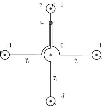
Figure 2. Generators of the fundamental group $\pi_{1}(B,t_{0})$.

Remark 4.9.

Note that the matrix $M^{\infty}$ is unipotent of maximal index $3$, i.e.

$$(M^{\infty}-1)^{3}=0,\quad(M^{\infty}-1)^{2}\neq 0$$

this will be crucial for the characterization of the period map in section 4.6.

The proof is a consequence of the following theorems.

Theorem 4.10 (Dolgachev [Dol96]).

The Dwork family $X\rightarrow B$ carries an $M_{2}$-polarization, i.e. there exists a morphism of local systems

(6) $$Pol:M_{2}\otimes\underline{{\mathbb{Z}}}_{B}\longrightarrow\mathcal{H}_{\mathbb{Z}}$$

inducing a primitive lattice embedding in each fiber which factorizes through the inclusion $\mathrm{Pic}(X_{t})\subset H^{2}(X_{t},{\mathbb{Z}})$. Moreover, for general $t$ this map is an isomorphism onto the Neron–Severi group.

Theorem 4.11 (Narumiyah–Shiga [NS01]).

There is a primitive lattice embedding

$$Tr:T_{0}\longrightarrow H^{2}(X_{t_{0}},{\mathbb{Z}})$$

with image in the orthogonal complement of the polarization $Pol(M_{2})_{t_{0}}$. Moreover the monodromy representation on $T_{0}$ is given by the matrices described in Theorem (4.8).

Proof.

The intersection form is stated in Theorem 4.1 of [NS01], and the monodromy matrices in Remark 4.2 following this theorem. We only explain how their notation differs form ours.

They consider the family $\tilde{F}_{\lambda}\subset{\mathbb{P}}^{3}$ defined by the equation

$$X_{0}^{4}+X_{1}^{4}+X_{2}^{4}+X_{3}^{4}+\lambda X_{0}X_{1}X_{2}X_{3}=0.$$

In order to ensure the relation $\lambda=4t$ holds, we identify this family via the isomorphism

$$\tilde{F}_{\lambda}\rightarrow F_{t},\quad X_{0}\mapsto-X_{0},\,X_{1}\mapsto X_{1},\,X_{2}\mapsto X_{2},\,X_{3}\mapsto X_{3}$$

with our Fermat pencil.

Their basis $(e^{\prime},f^{\prime},h^{\prime})$ of $U\oplus\langle 4\rangle$ is related to our basis $(h,e,f)$ of $\langle 4\rangle\oplus U$ by

$$(h,e,f)=(e^{\prime},f^{\prime},h^{\prime}).T,\quad T:=\begin{pmatrix}0&1&0\\ 0&0&1\\ 1&0&0\end{pmatrix}$$

They introduce a new variable $t^{\prime}=-(\lambda)^{2}/2$ and consider paths $\delta_{1},\dots,\delta_{3}$ in the $t^{\prime}$-plane (Fig.6 in [NS01]). The images of our paths $\gamma_{1},\dots,\gamma_{4}$ are give by

$$\gamma_{1}\mapsto\delta_{1},\quad\gamma_{2}\mapsto\delta_{2}^{-1}\cdot\delta_{3}\cdot\delta_{2},\quad\gamma_{3}\mapsto\delta_{2}^{-1}\cdot\delta_{1}\cdot\delta_{2},\quad\gamma_{4}\mapsto\delta_{3}.$$

Let $N_{i}$ be the monodromy matrices along $\delta_{i}$ as stated in Remark 4.2 of [NS01]. By what was said above, we compute the monodromy matrix e.g. along $\gamma_{2}$ as

$$M^{2}=T^{-1}.(N_{2})^{-1}.N_{3}.(N_{2}).T.\qed$$

So far we do not know whether the primitive embedding

$$Pol_{t_{0}}\oplus Tr:M_{2}\oplus T_{0}\longrightarrow H^{2}(X_{t_{0}},{\mathbb{Z}})$$

can be extended to an isomorphism of lattices $\Lambda\longrightarrow H^{2}(X_{t_{0}},{\mathbb{Z}})$.

The following theorem of Nikulin ensures, that we can always change $Pol_{t_{0}}$ by an automorphism of $M_{2}$ such, that an extension exists.

Theorem 4.12 (Nikulin [Nik79], 1.14.4).

Let $i:S\rightarrow L$ be a primitive embedding of an even non-degenerate lattice $S$ of signature $(s_{+},s_{-})$ into an even non-degenerate lattice of signature $(l_{+},l_{-})$. For any other primitive embedding $j:S\rightarrow L$, there is an automorphism $\alpha\in O(L)$ such that $i=j\circ\alpha$ if

$$l_{+}>s_{+},l_{-}>s_{-}\quad\text{and}\quad rk(L)-rk(S)\geq l(S)+2$$

where $l(S)$ is the minimal number of generators of the discriminant group $S^{\vee}/S$.

We apply this theorem as follows. First choose an arbitrary isomorphism $\tilde{n}:\Lambda\rightarrow H^{2}(X_{t_{0}},{\mathbb{Z}})$. This gives us a primitive embedding of $T_{0}$ by restriction

$$\tilde{n}|_{T_{0}}:T_{0}\longrightarrow H^{2}(X_{t_{0}},{\mathbb{Z}}).$$

Also there is the primitive embedding constructed in (4.11)

$$Tr:T_{0}\longrightarrow H^{2}(X_{t_{0}},{\mathbb{Z}}).$$

Note that $sign(T_{0})=(2,1),sign(\Lambda)=(3,19)$ and $l(T_{0})=l(\langle 4\rangle)=1$, so we can apply Nikulin’s theorem to conclude, that these two differ by an orthogonal automorphism $\alpha$ of $H^{2}(X_{t_{0}},{\mathbb{Z}})$.

Set $n=\alpha\circ\tilde{n}$ so that $\tilde{n}|_{T_{0}}=Tr$. Note also that $n$ induces an isomorphism of the orthogonal complements

$$n|_{M_{2}}:M_{2}=T_{0}^{\perp}\longrightarrow Tr(T_{0})^{\perp}=Pol(M_{2})_{t_{0}}.$$

As mentioned above, this isomorphism can differ, by an automorphism of $M_{2}$, from the one provided by Dolgachev’s polarization. It is now clear that $m=n^{-1}$ is a marking with the required properties. This concludes the proof of Theorem 4.8. ∎

Corollary 4.13.

The local system $\mathcal{H}_{\mathbb{Q}}:=\mathcal{H}_{\mathbb{Z}}\otimes{\mathbb{Q}}$ decomposes into an orthogonal direct sum

$$\mathcal{H}_{\mathbb{Q}}=\mathcal{P}_{\mathbb{Q}}\oplus\mathcal{T}_{\mathbb{Q}}$$

where $\mathcal{P}_{\mathbb{Q}}$ is a trivial local system of rank $19$ spanned by the algebraic classes in the image of the polarization $Pol$, and $\mathcal{T}_{\mathbb{Q}}$ is spanned by the image of $Tr$.

4.4. The Picard–Fuchs equation

So far we have described the local system $\mathcal{H}_{\mathbb{Z}}$ and the Hodge filtration ${\mathcal{F}}^{i}\subset\mathcal{H}$ of the Dwork family independently. The next step is to relate them to each other by calculating the period integrals

$$t\mapsto\int_{\Gamma}\Omega_{t}$$

for local sections $\Gamma\in\mathcal{H}_{\mathbb{Z}}$. The essential tool here is a differential equation, the Picard–Fuchs equation, that is satisfied by these period integrals.

Let $t$ be the affine coordinate on $B\subset{\mathbb{A}}^{1}$, and $\partial_{t}$ the associated global vector field. The Gauß–Manin connection $\nabla$ on $\mathcal{H}=\mathcal{H}_{\mathbb{Z}}\otimes{\mathcal{O}}_{B}$ is defined by $\Gamma\otimes f\mapsto\Gamma\otimes df$. We denote by

$$\Omega^{(i)}:=\nabla_{\partial_{t}}\circ\dots\circ\nabla_{\partial_{t}}\Omega\;\in\;H^{0}(B,\mathcal{H})$$

be the $i$-th iterated Gauß–Manin derivative of $\Omega$ in direction $\partial_{t}$.

Proposition 4.14.

The global section $\Omega$ of $\pi_{*}\Omega^{2}_{X/B}$ satisfies the differential equation

(7) $$\Omega^{(3)}=\frac{1}{1-t^{4}}(6t^{3}\Omega^{(2)}+7t^{2}\Omega^{(1)}+t\Omega).$$

Proof.

This is an application of the Griffiths–Dwork reduction method, see [Gri69], or [Mor92] for a similar application. We will outline the basic steps.

It is enough to prove the formula on the dense open subset $\rho(S_{t}^{reg})$ of $X$. Since the map $F\rightarrow S$ is étale over $S_{t}^{reg}$, we can furthermore reduce the calculation to the Fermat pencil of quartic hypersurfaces. The holomorphic forms on the members $F_{t}$ of the Fermat pencil are residues of meromorphic 3-forms $\Xi_{t}$ on ${\mathbb{P}}^{3}$. Since taking residues commutes with the Gauß–Manin connection, we only need to differentiate the global 3-from $\Xi_{t}$.

We then use a criterion of Griffiths to show the corresponding equality between the residues. This involves a Gröbner basis computation in the Jacobi ring of $F_{t}$. See e.g. [Smi07] for an implementation. ∎

Definition 4.15.

We define the Picard–Fuchs operator associated to the Dwork family $X\rightarrow B$ to be the differential operator

(8) $$\mathcal{D}=\partial_{t}^{3}-\frac{1}{1-t^{4}}(6t^{3}\partial_{t}^{2}+7t^{2}\partial_{t}+t)$$

obtained from (7) by replacing $\nabla$ with $\partial_{t}$.

Remark 4.16.

Let $\Gamma_{t}\in H^{2}(X_{t},{\mathbb{Z}})$ be a cohomology class. Extend $\Gamma_{t}$ to a flat local section $\Gamma$ of $\mathcal{H}_{\mathbb{Z}}$. Since the quadratic form $(\,.\,)$ on $\mathcal{H}_{\mathbb{Z}}$ is also flat, we can calculate

$$\partial_{t}\langle\Gamma,\Omega\rangle=\langle\Gamma,\nabla_{\partial_{t}}\Omega\rangle=\langle\Gamma,\Omega^{(1)}\rangle.$$

Similarly one finds that the function

$$t\mapsto\int_{\Gamma_{t}}\Omega_{t}=\langle\Gamma,\Omega\rangle(t)$$

is a solution of the Picard–Fuchs equation $\mathcal{D}=0$.

4.5. The period map of the Dwork family

Recall that the Dwork family

$$\pi:X\longrightarrow B,\quad B={\mathbb{P}}^{1}\setminus\Sigma,\quad\Sigma=\{t\,|\,t^{4}=1\}\cup\infty$$

determines a variation of Hodge structures on $B$:

$$\mathcal{H}_{\mathbb{Z}}:=R^{2}\pi_{*}\underline{{\mathbb{Z}}}_{X},\quad{\mathcal{F}}^{2}=\pi_{*}\Omega^{2}_{X/B}\;\subset\;{\mathcal{F}}^{1}=({\mathcal{F}}^{2})^{\perp}\;\subset\;\mathcal{H}:=\mathcal{H}_{\mathbb{Z}}\otimes{\mathcal{O}}_{B}.$$

We let $c:\tilde{B}\rightarrow B$ be the universal cover, and choose a point $\tilde{t_{0}}\in\tilde{B}$ mapping to $t_{0}=i/\sqrt{2}$.

Proposition 4.17.

The isomorphism constructed in Theorem 4.8

$$m:H^{2}(X_{t_{0}},{\mathbb{Z}})\longrightarrow\Lambda$$

induces a marking of the local system $c^{*}\mathcal{H}_{\mathbb{Z}}$.

Proof.

We compose $m$ with the canonical isomorphisms

$$(c^{*}\mathcal{H}_{\mathbb{Z}})_{\tilde{t_{0}}}\longrightarrow(\mathcal{H}_{\mathbb{Z}})_{t_{0}}\longrightarrow H^{2}(X_{t_{0}},{\mathbb{Z}})$$

and extend this map by parallel transport to an isomorphism of local systems

$$m:c^{*}\mathcal{H}_{\mathbb{Z}}\longrightarrow\underline{{\mathbb{Z}}}_{\tilde{B}}\otimes\Lambda.$$

This is possible since $\tilde{B}$ is simply connected, and hence both local systems are trivial. ∎

Choosing the marking in this way we get a period map

$$\mathscr{P}:=\mathscr{P}(c^{*}\mathcal{F}^{*},m):\tilde{B}\longrightarrow\mathscr{D}(\Lambda).$$

Proposition 4.18.

Let $M_{2},T_{0}\subset\Lambda$ be as in Theorem 4.8. The period map takes values in $\mathscr{D}(T_{0})\subset\mathscr{D}(\Lambda)$.

Proof.

Let $D\in\mathcal{H}_{\mathbb{Z}}$ be a local section contained in the orthogonal complement $m^{-1}(M_{2})$ of $m^{-1}(T_{0})$. By Dolgachev’s theorem 4.10, $D$ is fiber-wise contained in the Picard group, hence $(D.\Omega)=0$ by orthogonality of the Hodge decomposition. ∎

Let $(h,e,f)$ be the standard basis of $T_{0}=\langle 4\rangle\oplus U$, we denote by the same symbols also the global sections of $c^{*}\mathcal{H}_{\mathbb{Z}}$ associated via the marking. By the last proposition we find holomorphic functions $a,b,c$ on $\tilde{B}$ such that

(9) $$c^{*}\Omega=a\,h+b\,e+c\,f\;\in\,H^{0}(\tilde{B},c^{*}\mathcal{H})$$

and hence

$$\mathscr{P}=[a:b:c]:\tilde{B}\longrightarrow{\mathbb{P}}(T_{0})\subset{\mathbb{P}}(\Lambda\otimes{\mathbb{C}}),$$

using the abusive notation $[a:b:c]:=[ah+be+cf]$.

Remark 4.19.

For each point $\tilde{p}\in\tilde{B},\;p=c(\tilde{p})$ there is a canonical isomorphism of stalks

$$c^{*}:{\mathcal{O}}_{B,p}\longrightarrow{\mathcal{O}}_{\tilde{B},\tilde{p}},\quad f\mapsto f\circ c.$$

In this way we may view functions on $\tilde{B}$ locally (on $\tilde{B}$) as functions on $B$.

Proposition 4.20.

If we view the functions $a,b,c$ locally as functions on $B$, then these functions satisfy the Picard–Fuchs equation (8).

Proof.

We can express $a,b,c$ as intersections with the dual basis in the following way. If $(h^{\vee},e^{\vee},f^{\vee})=(h,e,f).G^{-1}=(1/4h,f,e)$, where $G$ is the Gram matrix of $(\,.\,)$ on the basis $(h,e,f)$, i.e.

$$G=\begin{pmatrix}4&0&0\\ 0&0&1\\ 0&1&0\end{pmatrix},$$

then $a=(h^{\vee}.\Omega),b=(e^{\vee}.\Omega)$ and $c=(f^{\vee}.\Omega).$ This exhibits the functions $a,b,c$ as period integrals and therefore shows that they satisfy the Picard–Fuchs equation. ∎

Proposition 4.21.

The germs of the functions $a,b,c$ at $\tilde{p}$ form a basis for the three-dimensional vector space $Sol(\mathcal{D},p)\subset{\mathcal{O}}_{B,p}$ of solutions of the Picard–Fuchs equation for all $\tilde{p}\in\tilde{B}$.

Proof.

Linear independence of $a,b,c$ is equivalent to the non-vanishing of the Wronski determinant

$$W=det\begin{pmatrix}a&b&c\\ \partial_{t}a&\partial_{t}b&\partial_{t}c\\ \partial_{t}^{2}a&\partial_{t}b&\partial_{t}^{2}c\end{pmatrix}$$

of this sections. As the differential equation (8) is normalized, this determinant is either identically zero or vanishes nowhere. If the vectors are everywhere linearly dependent, then we get a relation between the Gauß–Manin derivatives $\Omega,\Omega^{(1)},\Omega^{(2)}$, since

$$\Omega^{(1)}=\nabla_{\partial t}\Omega=(\partial_{t}a)\,h+(\partial_{t}b)\,e+(\partial_{t}c)\,f.$$

This means, that there is a order-two Picard–Fuchs equation for our family. That this is not the case, follows directly from the Griffiths–Dwork reduction process (Proposition 4.14). ∎

4.6. Characterization of the period map via monodromies

We have seen, that the coefficients of the period map satisfy the Picard–Fuchs equation. In this section we characterize these functions among all solutions. The key ingredient is the monodromy calculation in Theorem 4.8.

Remark 4.22.

We briefly explain how analytic continuation on $B$ is related to global properties of the function on the universal cover $\tilde{B}$ and thereby introduce some notation.

Let $\tilde{p}$ be a point in $\tilde{B}$, mapping to $p=c(\tilde{p})\in B$ and let $\delta:p\rightarrow q$ be a path in $B$. There is a unique lift of $\delta$ to $\tilde{B}$ starting at $\tilde{p}$. Denote this path by $\tilde{\delta}:\tilde{p}\rightarrow\tilde{q}$ and define $\delta\cdot\tilde{p}:=\tilde{q}$.

Also we can analytically continue holomorphic functions along $\delta$, this gives us a partially defined morphism between the stalks

$$AC_{\delta}:{\mathcal{O}}_{B,p}\longrightarrow{\mathcal{O}}_{B,q}.$$

A theorem of Cauchy [Inc44] ensures that if a function satisfies a differential equation of the form (8), then it can be analytically continued along every path.

These two constructions are related as follows. Let $f:\tilde{B}\rightarrow{\mathbb{C}}$ be a holomorphic function. We can analytically continue the germ $f_{\tilde{p}}\in{\mathcal{O}}_{B,p}$ along $\delta$ and get $AC_{\delta}f_{\tilde{p}}=f_{\tilde{q}},\;\tilde{q}=\delta\cdot\tilde{p}$.

Suppose now, that $\delta$ has the same start and end point $t_{0}=i/\sqrt{2}\in B$. We can express the analytic continuation of $\mathscr{P}$ along this paths in terms of the monodromy matrices of $\mathcal{H}_{\mathbb{Z}}$.

Proposition 4.23.

Let $\delta\in\pi_{1}(B,t_{0})$ and

$$PT_{\delta}(h,e,f)=(h,e,f).M^{\delta}$$

be the monodromy representation of the local system $\mathcal{H}_{\mathbb{Z}}$ as in Theorem 4.8. The analytic continuation of the period map at $\tilde{t_{0}}$ is given by

$$AC_{\delta}\mathscr{P}_{\tilde{t_{0}}}=AC_{\delta}[a:b:c]=[a^{\prime}:b^{\prime}:c^{\prime}]$$

as tuple of germs at $\tilde{t_{0}}$, where

$$(a^{\prime},b^{\prime},c^{\prime})=(a,b,c).G.M^{\delta}.G^{-1}$$

Proof.

As remarked above we have the identity of tuples of functions on $\tilde{B}$

$$(a,b,c)=((h^{\vee},e^{\vee},f^{\vee}).\Omega(p))=(\_.\Omega)\circ(h,e,f).G^{-1}.$$

Now integrals of the form $\int_{\Gamma(\tilde{p})}\Omega(p)=(\Gamma.\Omega)(\tilde{p})$ can be analytically continued by transporting the cycle $\Gamma$ in the local system. Thus we conclude

$$AC_{\delta}(a,b,c) =AC_{\delta}(\_.\Omega)\circ(h,e,f).G^{-1}=(\_.\Omega)\circ(PT_{\delta}(h,e,f)).G^{-1}$$

$$=(\_.\Omega)\circ(h,e,f).M^{\delta}.G^{-1}=(a,b,c).G.M^{\delta}.G^{-1}.\qed$$

We already saw in Proposition 3.2 that the period domain $\mathscr{D}(\langle 4\rangle\oplus U)=\mathscr{D}(T_{0})$ is isomorphic to ${\mathbb{C}}\setminus{\mathbb{R}}$. Let $(h,e,f)$ be the standard basis of $\langle 4\rangle\oplus U$. A slightly different isomorphism is given by

(10) $$\tilde{exp}:{\mathbb{C}}\setminus{\mathbb{R}}\longrightarrow\mathscr{D}(T_{0}),\;z \mapsto[z\,h\,-\,1\,e\,+\,2z^{2}\,f]$$

with inverse $\tilde{exp}^{-1}:[a\,h\,+\,b\,e\,+\,c\,f]\mapsto-a/b$.

We consider the period map as a function to the complex numbers using this parametrization of the period domain:

$$\mathscr{P}^{c}=\tilde{exp}^{-1}\circ\mathscr{P}:\tilde{B}\longrightarrow{\mathbb{C}}.$$

We will see later, that the period map takes values in the upper half plane.

Theorem 4.8 has a translation into properties of this function.

Proposition 4.24.

The analytic continuation of the germ of the period map at $\tilde{t_{0}}$ along the paths $\gamma_{k}$ depicted in Figure 2 is given by

$$AC_{\gamma_{k}}\mathscr{P}^{c}_{\tilde{t_{0}}}=\beta_{k}(\mathscr{P}^{c}_{\tilde{t_{0}}})$$

where $\beta_{k}:{\mathbb{H}}\rightarrow{\mathbb{H}}$ are the Möbius transformations:

$$\beta_{1}(z)=\frac{-1}{2z},\;\beta_{2}(z)=\frac{1-2z}{2-6z},\;\beta_{3}(z)=\frac{3-4z}{4-6z},\;\beta_{4}(z)=\frac{3-2z}{2-2z},$$

$$\beta_{\infty}(z)=4+z.$$

Proof.

Direct calculation using Proposition 4.23. ∎

The modification (10) of the parametrization was introduced to bring the monodromy at infinity to this standard form.

The fixed points of $\beta_{i}$ are

(11) $$\beta_{1}:\pm i/\sqrt{2},\;\;\beta_{2}:\frac{1}{3}(1\pm i/\sqrt{2}),\;\;\beta_{3}:\frac{1}{3}(2\pm i/\sqrt{2}),\;\;\beta_{4}:1\pm i/\sqrt{2}.$$

These are also the limiting values of the period map at the corresponding boundary points $i,-1,-i,1\in{\mathbb{P}}^{1}\setminus B$.

The following characterization of the period map in terms of monodromies is crucial. We show that the period map is determined up to a constant by the monodromy at a maximal unipotent point (cf. Remark 4.9). This is similar to the characterization of the mirror map by Morrison [Mor92, Sec. 2]. The remaining constant can be fixed by considering an additional monodromy transformation.

Proposition 4.25.

Let $a^{\prime},b^{\prime}\in{\mathcal{O}}_{t_{0}}$ be non-zero solutions to the Picard–Fuchs equation and $\mathscr{P}^{\prime}:=a^{\prime}/b^{\prime}$. If

$$AC_{\gamma_{\infty}}(a^{\prime},b^{\prime})=(a^{\prime},b^{\prime}).\begin{pmatrix}1&0\\ 4&1\end{pmatrix},\quad$$

then there is a $\mu\in{\mathbb{C}}$ such that $\mathscr{P}^{\prime}=\mathscr{P}^{c}+\mu$ as germs at $\tilde{t_{0}}$.

If furthermore

$$AC_{\gamma_{1}}\mathscr{P}^{\prime}=\beta(\mathscr{P}^{\prime})$$

for a Möbius transformation $\beta$ with fixed points $\pm i/\sqrt{2}$, then $\mathscr{P}^{\prime}=\mathscr{P}^{c}$.

Proof.

By Proposition 4.21 the functions $a^{\prime},b^{\prime}$ are a ${\mathbb{C}}$-linear combination of $a,b,c$. The monodromy transformation of $(a,b,c)$ at infinity is

$$N^{\infty}:=G.M^{\infty}.G^{-1}=\begin{pmatrix}1&0&16\\ -4&1&-32\\ 0&0&1\end{pmatrix}.$$

Note that $a,b$ have the same monodromy behavior as $-a^{\prime},b^{\prime}$ at infinity. The matrix $N^{\infty}$ is unipotent of index $3$, i.e. $(N^{\infty}-{\rm id})^{3}=0,\,(N^{\infty}-{\rm id})^{2}\neq 0$. In particular the only eigenvalue is $1$ and the corresponding eigenspace is one-dimensional, spanned by $e_{2}=(0,1,0)^{t}$. Hence there is a $\lambda\in{\mathbb{C}}$ such that $b^{\prime}=\lambda b$.

The vector $v=(1,0,0)^{t}$ is characterized by the property $(N^{\infty}-1)v=-4e_{2}$. The space of such $v$ is a one dimensional affine space over the eigenspace ${\mathbb{C}}\,e_{2}$. We conclude that $-a^{\prime}=\lambda a-\mu b$, for some $\mu\in{\mathbb{C}}$. Since $b\neq 0$ it is $\lambda\neq 0$ and we may assume $\lambda=1$. Hence

$$\mathscr{P}^{\prime}=a^{\prime}/b^{\prime}=-a/b+\mu=\mathscr{P}^{c}+\mu.$$

Moreover the monodromy of this function along $\gamma_{1}$ is

$$AC_{\gamma_{1}}\mathscr{P}^{\prime}=AC_{\gamma_{1}}\mathscr{P}^{c}+\mu=\beta_{1}(\mathscr{P}^{c})+\mu.$$

The fixed point equation $\beta_{1}(z)+\mu=z$ is a polynomial of degree $2$ with discriminant $-2+\mu^{2}$. This means the difference of the two solution is $i\sqrt{2}$ only if $\mu=0$. ∎

4.7. Nagura and Sugiyama’s solutions

Solutions to the Picard–Fuchs equation matching the criterion 4.25 were produced by Nagura and Sugiyama in [NS95]. To state their result, we first need to transform the equation.

The first step is to change the form $\Omega$ to $t^{-1}\Omega$, which does not affect the period map, but changes the Picard–Fuchs equation from $\mathcal{D}=0$ to $\mathcal{D}.t=0$. We can further multiply by $(1-t^{4})$ from the left, without changing the solution space. This differential equation now does descend along the covering map

$$z:B\setminus\{0\}\longrightarrow{\mathbb{P}}^{1}\setminus\{0,1,\infty\},\quad t\mapsto z(t)=t^{-4}$$

to a hypergeometric system on $C$.

Proposition 4.26.

Let

(12) $$_{3}\mathcal{D}_{2}:=\vartheta^{3}-z(\vartheta+1/4)(\vartheta+2/4)(\vartheta+3/4),\quad\vartheta=z\partial_{z}$$

be the differential operator on ${\mathbb{P}}^{1}\setminus\{0,1,\infty\}$ associated to the generalized hypergeometric function ${}_{3}F_{2}(1/4,2/4,3/4;1;1;u)$ then

$$z^{*}_{3}\mathcal{D}_{2}=\frac{1}{64}(1-t^{4}).\mathcal{D}.t.$$

Proof.

Direct calculation. ∎

Example 4.27.

The function on $B$

$${}_{3}F_{2}(\frac{1}{4},\frac{2}{4},\frac{3}{4};1;1;t^{-4})t$$

defined for $|t|>1$ satisfies the Picard–Fuchs equation.

Consider the solutions to the hypergeometric differential equation ${}_{3}\mathcal{D}_{2}$

$$W_{1}(z) =\sum_{n=0}^{\infty}\frac{(4n)!}{(n!)^{4}(4^{4})^{n}}z^{n}=_{3}F_{2}(\frac{1}{4},\frac{2}{4},\frac{3}{4};1,1;z)$$

$$W_{2}(z) =\ln(4^{-4}z)W_{1}(z)+4\sum_{n=0}^{\infty}\frac{(4n)!}{(n!)^{4}(4^{4})^{n}}[\Psi(4n+1)-\Psi(n+1)]z^{n}.$$

where $\Psi$ denotes the digamma-function $\Psi(z)=\Gamma^{\prime}(z)/\Gamma(z)$. The functions $W_{i}(t^{-4}),i=1,2$ are solutions to the pulled back equation $z^{*}_{3}\mathcal{D}_{2}$. We set

$$P(t):=\frac{1}{2\pi i}\frac{W_{2}(t^{-4})}{W_{1}(t^{-4})}.$$

These functions converge for $|t|>1$ and hence define germs at the point $t_{1}=i\sqrt{2}$. The logarithm is chosen in such a way that $Im(\ln((4t_{1})^{-4}))=0$.

Choose a path $\delta:t_{0}\rightarrow t_{1},\,t_{0}=i/\sqrt{2},t_{1}=i\sqrt{2}$ within the contractible region $\{t\,|\,Re(t)>0,\,Im(t)>0\}\subset B$. We get an isomorphism between the fundamental groups by

$$T_{\delta}:\pi_{1}(B,t_{0})\rightarrow\pi_{1}(B_{,}t_{1}),\quad\gamma\mapsto\delta\cdot\gamma\cdot\delta^{-1}$$

The analytic continuation along $T_{\delta}\gamma_{\infty}$ can be read off the definition

$$AC_{T_{\delta}\gamma_{\infty}}W_{1}=W_{1},\quad AC_{T_{\delta}\gamma_{\infty}}W_{2}=W_{2}+4(2\pi i)W_{1}.$$

Indeed, the sums define holomorphic functions and are therefore unaffected by analytic continuation. The only contribution comes from the logarithmic term. The path $T_{\delta}\gamma_{\infty}$ encircles $\infty$ once with positive orientation. Therefore $0$ is encircled with negative orientation, so the logarithm picks up a summand $-2\pi i$.

We can apply the first part of criterion 4.25 to see

$$\mathscr{P}^{c}(t)=P(t)+\mu$$

as germs of functions at $\tilde{t_{1}}:=\delta\cdot\tilde{t_{0}}$ for some $\mu\in{\mathbb{C}}$. To apply the second part of the criterion we need the following additional information.

Theorem 4.28 (Nagura, Sugiyama [NS95]).

An analytic continuation of the map $P:=\frac{1}{2\pi i}W_{2}/W_{1}$ to a sliced neighborhood of $t=1$ is given by

$$P(t) =\frac{i}{\sqrt{2}}\frac{U_{1}(t)+\tan(\frac{\pi}{8})^{-1}U_{2}(t)}{U_{1}(t)-\tan(\frac{\pi}{8})^{-1}U_{2}(t)}$$

$$U_{1}(t) =\frac{\Gamma(\frac{1}{8})^{2}}{\Gamma(\frac{1}{2})}_{2}F_{1}(\frac{1}{8},\frac{3}{8};\frac{1}{2};1-t^{4})$$

$$U_{2}(t) =\frac{\Gamma(\frac{5}{8})^{2}}{\Gamma(\frac{3}{2})}(t^{4}-1)^{1/2}_{2}F_{1}(\frac{5}{8},\frac{5}{8};\frac{3}{2};1-t^{4}).$$

Thus the monodromy around the point $t=1$ satisfies $AC_{T_{\delta}\gamma_{4}}P=-\frac{1}{2P}$.

We find get following corollary.

Theorem 4.29.

The composition of the period map with the parametrization of the period domain (10)

$$\mathscr{P}^{c}=\tilde{exp}\circ\mathscr{P}:\tilde{B}\longrightarrow\mathscr{D}(T_{0})\longrightarrow{\mathbb{C}}\setminus{\mathbb{R}}$$

is explicitly given in a neighborhood of $\tilde{t_{1}}$ by

$$\mathscr{P}^{c}(t)=P(t)=\frac{1}{2\pi i}\frac{W_{2}(t^{-4})}{W_{1}(t^{-4})}.$$

Proof.

We have to check, that the function $P$ has the right analytic continuation along $T_{\delta}\gamma_{1}$, i.e. $AC_{T_{\delta}\gamma_{1}}P=-1/(2P)$. We know the analytic continuation of $P$ along $T_{\delta}\gamma_{4}$ has this form.

But $P$ only depends on $z=t^{-4}$ not on $t$ itself. Moreover the images of the paths $\gamma_{1}$ and $\gamma_{4}$ under $t\mapsto t^{-4}$ coincide. Hence also the analytic continuations are the same. ∎

Proposition 4.30.

The power series expansion of $\mathscr{P}^{c}$ at $t=\infty$ is given by

$$\mathscr{P}^{c}(w)=\frac{1}{2\pi i}(\ln(w)+104\,w+9780\,{w}^{2}+{4141760}/{3}\,{w}^{3}+231052570\,{w}^{4}+\dots)$$

$$exp(2\pi i\mathscr{P}^{c}(w))=w+104\,{w}^{2}+15188\,{w}^{3}+2585184\,{w}^{4}+480222434\,{w}^{5}+\dots$$

where $w=1/(4t)^{4}=4^{-4}z$.

This is precisely the series obtained by Lian and Yau [LY96] using a different method (see Remark 5.2). They also prove that the expansion of $exp(2\pi i\mathscr{P}^{c}(w))$ has integral coefficients.

Corollary 4.31.

The period map $\mathscr{P}^{c}$ takes values in the upper half plane.

Remark 4.32.

We show how Theorem 1.2 stated in the introduction can be derived from 4.29.

We identify $H^{2}(X_{t_{0}},{\mathbb{Z}})\cong\Lambda$ via the isomorphism given in Theorem 4.8 and use parallel transport to extend this isomorphism to nearby fibers $X_{t}$.

The period vector $\Omega_{t}$ is contained in $T_{0}\otimes{\mathbb{C}}$, where $T_{0}=\langle 4\rangle\oplus U\subset\Lambda$ is the generic transcendental lattice. By Theorem 4.29 and (10) we have

$$[\Omega_{t}]=[\tilde{exp}(\mathscr{P}^{c}(t))]\in{\mathcal{D}}(T_{0})\subset{\mathbb{P}}(\Lambda_{\mathbb{C}})$$

and hence there is a nowhere vanishing holomorphic function $f(t)$ such that

(13) $$f(t)\Omega_{t}=\tilde{exp}(\mathscr{P}^{c}(t))=\mathscr{P}^{c}(t)h-e+2(\mathscr{P}^{c}(t))^{2}f.$$

As $f(t)\Omega_{t}$ is also a non-vanishing holomorphic two-form we can assume this equation holds true already for $\Omega_{t}$. The period integrals can now be calculated as intersection products $\int_{\Gamma}\Omega_{t}=\Omega_{t}.\Gamma$.

The required basis $\Gamma_{i}$ of $\Lambda=2E_{8}(-1)\oplus U^{\prime\prime}\oplus U^{\prime}\oplus U$ is constructed as follows. We let $(\Gamma_{1},\Gamma_{2},\Gamma_{3})=(h,e,f)$ be the standard basis of $T_{0}$. Recall that $h=e^{\prime}+2f^{\prime}$ and hence $(\Gamma_{1},\Gamma_{4})=(h,f^{\prime})$ is a basis of $U^{\prime}$. The remaining basis vectors can be chosen to be any basis of the orthogonal complement $2E_{8}(-1)\oplus U^{\prime\prime}$ of $(\Gamma_{1},\dots,\Gamma_{4})$. Using (13) it is now straightforward to calculate the entries of the period vector.

4.8. The period map as Schwarz triangle function

In this section we will relate the period map to a Schwarz triangle function. We begin by recalling some basic facts about these functions from [Beu07].

Definition 4.33.

The hypergeometric differential equation with parameters $a,b,c\in{\mathbb{C}}$ is

(14) $$\vartheta(\vartheta+c-1)f-z(\vartheta+a)(\vartheta+b)f=0,\quad\vartheta=z\partial_{z},\,f\in{\mathcal{O}}_{\mathbb{C}}$$

which is satisfied by the hypergeometric function $f=_{2}F_{1}(a,b;c;z)$.

Let $f,g$ be two independent solutions to this differential equation at a point $z_{0}\in{\mathbb{H}}$. The function $D(z)=f/g$ considered as map ${\mathbb{H}}\rightarrow{\mathbb{C}}$ is called Schwarz triangle function.

These functions have very remarkable properties and were studied extensively in the 19th century (see Klein’s lectures [Kle33]).

Definition 4.34.

A curvilinear triangle is an open subset of ${\mathbb{P}}^{1}$ whose boundary is the union of three open segments of circles or lines and three points. The segments are called edges and the points vertices of the triangle.

Proposition 4.35.

For any three distinct points $A,B,C\in{\mathbb{P}}^{1}$ and positive, real numbers $\lambda,\mu,\nu$ with $\lambda+\mu+\nu<1$ there is a unique curvilinear triangle with vertices $(A,B,C)$ and interior angles $(\lambda\pi,\mu\pi,\nu\pi)$ in that order.

Theorem 4.36 (Schwarz, [Beu07] 3.20).

A Schwarz triangle function maps the closed upper half plane ${\mathbb{H}}\cup{\mathbb{R}}$ isomorphically to a curvilinear triangle.

The vertices are the points $(D(0),D(1),D(\infty))$ and the corresponding angles $(\lambda\pi,\mu\pi,\nu\pi)$ depend on the parameters of the hypergeometric differential equation via $\lambda=|1-c|,\mu=|c-a-b|,\nu=|a-b|$.

Recall that the period map is a function on the universal cover of $B={\mathbb{P}}^{1}\setminus\Sigma$ to the upper half plane.

$$\mathscr{P}^{c}:\tilde{B}\longrightarrow{\mathbb{H}}.$$

This maps descends along $t\mapsto z(t)=t^{-4}$ to a multi-valued map on ${\mathbb{P}}^{1}\setminus\{0,1,\infty\}$. We explain this last sentence more formally. The map $t\mapsto z(t)=t^{-4}$ is an unramified covering $B\setminus\{0\}\rightarrow{\mathbb{P}}^{1}\setminus\{0,1,\infty\}$. Hence it induces an isomorphism between the universal covering spaces. Moreover the inclusion $B\setminus\{0\}\rightarrow B$ induces a map $(B\setminus\{0\})\widetilde{\phantom{X}}\rightarrow\tilde{B}$. We use the composition

$$({\mathbb{P}}^{1}\setminus\{0,1,\infty\})\widetilde{\phantom{X}}\cong(B\setminus\{0\})\widetilde{\phantom{X}}\longrightarrow\tilde{B}$$

to view $\mathscr{P}^{c}:\tilde{B}\rightarrow{\mathbb{H}}$ as multi-valued map on ${\mathbb{P}}^{1}\setminus\{0,1,\infty\}$.

We choose a basepoint $\tilde{z}_{1}$ of $({\mathbb{P}}^{1}\setminus\{0,1,\infty\})\widetilde{\phantom{X}}$ mapping to $\tilde{t_{1}}$. Denote by $\iota$ the unique lift of the inclusion ${\mathbb{H}}\rightarrow{\mathbb{P}}^{1}\setminus\{0,1,\infty\}$ to the universal cover of ${\mathbb{P}}^{1}\setminus\{0,1,\infty\}$ mapping $z_{1}$ to $\tilde{z}_{1}$ (when extended to the boundary of ${\mathbb{H}}\subset B$).

Theorem 4.37.

The restriction of the period map

$$\mathscr{P}^{c}(z):({\mathbb{P}}^{1}\setminus\{0,1,\infty\})\widetilde{\phantom{X}}\longrightarrow{\mathbb{P}}^{1}$$

to $\iota:{\mathbb{H}}\rightarrow({\mathbb{P}}^{1}\setminus\{0,1,\infty\})\widetilde{\phantom{X}}$ is a Schwarz triangle function. The upper half plane is mapped to the triangle with vertices $(\infty,\frac{i}{2},\frac{1+i}{2})$ and angles $(0,\pi/2,\pi/4)$ as pictured in Figure 1 in the introduction.

Proof.

The strategy is the following. We first construct the a triangle function with the expected mapping behavior. Then we write this function as a quotient of solution of the Picard–Fuchs equation. Finally we show that the assumptions of Proposition 4.25 are satisfied by this function. It follows that it has to be the period map.

Step 1. Let $f,g$ be two independent solutions to ${}_{2}\mathcal{D}_{1}$ at $t_{1}$. By Schwarz’ theorem $D(z)=f/g$ is a triangle function. Using a Möbius transformation, we can change the vertices of the triangle to be $(0,1,\infty)$. As the composition is again of the form $f^{\prime}/g^{\prime}$ for independent solutions $f^{\prime},g^{\prime}$ of ${}_{2}\mathcal{D}_{1}$ we can assume $D(z)$ maps $(0,1,\infty)$ to $(\infty,\frac{i}{\sqrt{2}},\frac{1+i}{2})$.

The triangle pictured in green color in Figure 1 is the unique curvilinear triangle with vertices $(\infty,\frac{i}{\sqrt{2}},\frac{1+i}{2})$ and interior angles $(0,\pi/2,\pi/4)$. Hence it is the image of ${\mathbb{H}}$ under $D(z)$.

The analytic continuation of $D(z)$ can be obtained by reflecting the triangle at its edges. This technique is called Schwarz reflection principle (see [Beu07] for details).

Let $\delta_{0},\delta_{1}\in\pi_{1}({\mathbb{P}}^{1}\setminus\{0,1,\infty\},z_{1})$ be the paths pictured in Figure 3 encircling $0,1$ once with positive orientation respectively. Reflecting the triangles according to the crossings of the paths with the components of ${\mathbb{R}}\setminus\{0,1\}$ we find

$$AC_{\delta_{0}}D(z)=D(z)+1,\quad AC_{\delta_{1}}D(z)=\frac{-1}{2D(z)}.$$

This means that $AC_{\delta_{0}}(f/g)=(f+g)/g$ and since $f,g$ are independent we can conclude that there is a $\lambda\in{\mathbb{C}}^{*}$ such that

(15) $$AC_{\delta_{0}}(f,g)=(f,g).\begin{pmatrix}\lambda&0\\ \lambda&\lambda\end{pmatrix}.$$

The hypergeometric function ${}_{2}F_{1}(\frac{1}{8},\frac{3}{8};1;z)$ is a linear combination of the basis solutions $(f,g)$. Since it is holomorphic at $0$, the matrix (15) has to have the eigenvalue $1$ which is only the case if $\lambda=1$.

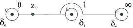
Figure 3. The paths $\delta_{i}$ in ${\mathbb{P}}^{1}\setminus\{0,1,\infty\}$ based at $z_{1}=1/4$.

Step 2. The ${}_{3}F_{2}$-hypergeometric function $W_{1}(z)$ occuring in the expansion of the period map is related to a ${}_{2}F_{1}$-hypergeometric function by the Clausen identity ([Bai35], p.86)

$${}_{3}F_{2}(\frac{1}{4},\frac{2}{4},\frac{3}{4};1;1;z)=_{2}F_{1}(\frac{1}{8},\frac{3}{8};z)^{2}.$$

The corresponding statement in terms of differential equations reads as follows.

Proposition 4.38.

The differential equation

(16) $$_{2}\mathcal{D}_{1}=\vartheta^{2}-z(\vartheta+1/8)(\vartheta+3/8),\quad\vartheta=z\frac{\partial}{\partial z}$$

associated to the hypergeometric function ${}_{1}F_{2}(\frac{1}{8},\frac{3}{8};1;z)$ has the property that for all solutions $f,g$ to ${}_{2}\mathcal{D}_{1}$ the product satisfies ${}_{3}\mathcal{D}_{2}(f.g)=0$.

Conversely any solution to ${}_{3}\mathcal{D}_{2}$ is a sum of products of solutions to ${}_{2}\mathcal{D}_{1}$.

Proof.

The proposition can be rephrased by saying ${}_{3}\mathcal{D}_{2}=Sym^{2}(_{2}\mathcal{D}_{1})$. There is an algorithm to compute such symmetric squares of differential operators, which is implemented e.g. in Maple. We used this program to verify the equality. ∎

Using this proposition and Proposition 4.26 we can trivially express $D(z)$ as a quotient of solutions of the Picard–Fuchs equation (8), namely

$$D(t^{-4})=\frac{f(t^{-4})}{g(t^{-4})}=\frac{f(t^{-4})g(t^{-4})\,t}{g(t^{-4})^{2}\,t}.$$

Step 3. We claim that the tuple $(a,b)=(f(t^{-4})g(t^{-4})\,t,g(t^{-4})^{2}\,t)$ of solutions of the Picard–Fuchs equation satisfies the assumptions of the criterion 4.25.

The paths $T_{\delta}\gamma_{\infty},T_{\delta}\gamma_{1}\in\pi_{1}(B,t_{1})$ in $B$ map to $\delta_{0}^{4},\delta_{1}\in\pi_{1}({\mathbb{P}}^{1}\setminus\{0,1,\infty\},z_{1})$ under $t\mapsto z(t)=t^{-4}$. Hence we can calculate the monodromy transformations as

$$AC_{T_{\delta}\gamma_{\infty}}(f,g)=(f,g).\begin{pmatrix}1&0\\ 1&1\end{pmatrix}^{4}=(f,g).\begin{pmatrix}1&0\\ 4&1\end{pmatrix}$$

and consequently also

$$AC_{T_{\delta}\gamma_{\infty}}(a,b)=(a,b).\begin{pmatrix}1&0\\ 4&1\end{pmatrix}$$

moreover

$$AC_{T_{\delta}\gamma_{1}}D(t^{-4})=\frac{-1}{2D(t^{-4})}$$

as required. This concludes the proof of the theorem. ∎

5. Mirror symmetries and mirror maps

It remains to translate the above computations in the framework developed in chapter 2.

Let $X\rightarrow B$ be the Dwork Pencil and

$$\mathscr{P}_{B}:\tilde{B}\longrightarrow\mathscr{D}(T_{0})\subset\mathscr{D}(\Lambda)\subset\mathscr{D}(\tilde{\Lambda})$$

the (B-model) period map associated to the marking, constructed in Theorem 4.8. Here $T_{0}\cong\langle h\rangle\oplus U$ is the transcendental lattice of the general member of $X/B$.

Let $\mathcal{Y}\rightarrow{\mathbb{H}}$ be the family of generalized K3 structures on a quartic $Y\subset{\mathbb{P}}^{3}$ as constructed in section 3 and

$$\mathscr{P}_{A}:{\mathbb{H}}\longrightarrow\mathscr{D}(\langle H\rangle\oplus U)\subset\mathscr{D}(\tilde{\Lambda})$$

the A-model period map as in Proposition 3.2. Here $\langle H\rangle\oplus U$ is the lattice spanned by the class of a hyperplane $H$ and $U\cong H^{0}\oplus H^{4}\subset\tilde{H}(Y,{\mathbb{Z}})$.

Theorem 5.1.

Mirror symmetry as described in Section 2.10 between the symplectic quartic in ${\mathbb{P}}^{3}$ and the Dwork family is determined by the diagram

where $g\in{\mathcal{O}}(\tilde{\Lambda})$ is a isometry interchanging $H^{0}\oplus H^{4}$ with $U\subset T_{0}$ and $\psi=\mathscr{P}^{c}$ is the period map of Theorem 4.29.

Proof.

Recall from 3.2 that $\mathscr{P}_{A}(z)=[1e+zH-2z^{2}f]$. On the other hand $\mathscr{P}^{c}$ was defined using the parametrization $\tilde{exp}(z)=[-1e+zh+2z^{2}f]$. So in order for the diagram to commute we should use the isometry

$$g_{0}:T_{0}=(\langle h\rangle\oplus U)\longrightarrow(\langle H\rangle\oplus U),\;h\mapsto H,e\mapsto-e,f\mapsto-f$$

to relate the period domains $\mathscr{D}(T_{0})$ and $\mathscr{D}((\langle H\rangle\oplus U))$. This isomorphism is easily seen to extend to an isometry g of $\tilde{\Lambda}$ using Nikulin’s theorem 4.12. ∎

Remark 5.2.

A period map in the sense of Morrison [Mor92] is a quotient $\psi=a/b$ of two solutions to the Picard–Fuchs equation $a,b$ satisfying the property

$$AC_{\gamma_{\infty}}\psi=\psi+1$$

for analytic continuation around the point of maximal unipotent monodromy. As in Proposition 4.25 one finds that $\psi$ is uniquely determined up to addition of a constant. One chooses this constant in such a way that the Fourier expansion at $\infty$ has integral coefficients.

Such a function can be constructed directly from the differential equation by using a Frobenius basis for the solutions at the singular point. Using this method, Lian and Yau [LY96] arrive at precisely the same formula 4.30.

There are several differences to our definition. First note, that our mirror maps are symmetries of the period domain of (generalized) K3 surfaces which become functions only after composition with the corresponding period maps.

Secondly and more importantly, we do require the solutions $a,b$ to be of the form $\int_{\Gamma}\omega_{t}$, for some integral cycle $\Gamma\in H^{2}(X_{t_{0}},{\mathbb{Z}})$. It is not clear (and in general not true) that the Frobenius basis has this property. This was the main difficulty we faced above. Our solution relied heavily on the work of Narumiyah and Shiga [NS01].

There is also a conceptual explanation that Morrison’s mirror map coincides with ours. Conjecturally (see [KKP08], [Iri09]) the Frobenius solutions differ form the integral periods by multiplication with the $\hat{\Gamma}$-class

$$\hat{\Gamma}(X)=\prod_{i=1}^{n}\Gamma(1+\delta_{i})=exp(-\gamma c_{1}(X)+\sum_{k\geq 2}(-1)^{k}(k-1)!\zeta(k)ch_{k}(TX))$$

where $\delta_{i}$ are the Chern roots of $TX$, $\gamma$ is Euler’s constant and $\zeta(s)$ is the Riemann zeta function. The Calabi–Yau condition $c_{1}(X)=0$ translates into the statement, that the first two entries of the Frobenius basis give indeed integral periods. In our case, this information suffices to fix the Hodge structure completely.

References

- [AM97] P. S. Aspinwall and D. R. Morrison. String theory on surfaces. In Mirror symmetry, II, volume 1 of AMS/IP Stud. Adv. Math., pages 703–716. Amer. Math. Soc., Providence, RI, 1997.
- [Bai35] W. N. Bailey. Generalized Hypergeometric Series. Cambridge University Press, 1935.
- [BBD85] A. Beauville, J.-P. Bourguignon, and M. Demazure. Géométrie des surfaces : modules et périodes. Société Mathématique de France, Paris, 1985.
- [Bel02] S.-M. Belcastro. Picard lattices of families of surfaces. Comm. Algebra, 30(1):61–82, 2002.
- [Beu07] F. Beukers. Gauss’ hypergeometric function. In Arithmetic and geometry around hypergeometric functions, volume 260 of Progr. Math., pages 23–42. Birkhäuser, Basel, 2007.
- [CMSP03] J. Carlson, S. Müller-Stach, and C. Peters. Period mappings and period domains, volume 85 of Cambridge Studies in Advanced Mathematics. Cambridge University Press, Cambridge, 2003.
- [COGP91] P. Candelas, X. de la Ossa, P. S. Green, and L. Parkes. A pair of Calabi-Yau manifolds as an exactly soluble superconformal theory. Nuclear Phys. B, 359(1):21–74, 1991.
- [Dol96] I. V. Dolgachev. Mirror symmetry for lattice polarized surfaces. J. Math. Sci., 81(3):2599–2630, 1996.
- [GH78] P. Griffiths and J. Harris. Principles of algebraic geometry. Wiley Classics Library. John Wiley & Sons Inc., New York, 1978.
- [Gri69] P. A. Griffiths. On the periods of certain rational integrals. I, II. Ann. of Math., 90:496–541, 1969.
- [Huy04] D. Huybrechts. Moduli spaces of hyperkähler manifolds and mirror symmetry. In Intersection theory and moduli, ICTP Lect. Notes, XIX, pages 185–247. Abdus Salam Int. Cent. Theoret. Phys., Trieste, 2004.
- [Huy05] D. Huybrechts. Generalized Calabi-Yau structures, surfaces, and -fields. Internat. J. Math., 16(1):13–36, 2005.
- [Inc44] E. L. Ince. Ordinary Differential Equations. Dover Publications, New York, 1944.
- [Iri09] H. Iritani. An integral structure in quantum cohomology and mirror symmetry for toric orbifolds. Preprint arXiv/0903.1463, 2009.
- [KKP08] L. Katzarkov, M. Kontsevich, and T. Pantev. Hodge theoretic aspects of mirror symmetry. In From Hodge theory to integrability and TQFT tt*-geometry, volume 78 of Proc. Sympos. Pure Math., pages 87–174. Amer. Math. Soc., Providence, RI, 2008.
- [Kle33] F. Klein. Vorlesungen über Hypergeometrische Funktionen. Springer-Verlag, Berlin, 1933.
- [Kon95] M. Kontsevich. Homological algebra of mirror symmetry. In Proceedings of the International Congress of Mathematicians, Vol. 1, 2 (Zürich, 1994), pages 120–139. Birkhäuser, Basel, 1995.
- [LY96] B. H. Lian and S.-T. Yau. Arithmetic properties of mirror map and quantum coupling. Comm. Math. Phys., 176(1):163–191, 1996.
- [Mor92] D. R. Morrison. Picard-Fuchs equations and mirror maps for hypersurfaces. In Essays on mirror manifolds, pages 241–264. Int. Press, Hong Kong, 1992.
- [Mos65] J. Moser. On the volume elements on a manifold. Trans. Amer. Math. Soc., 120:286–294, 1965.
- [Nik76] V. V. Nikulin. Finite groups of automorphisms of Kählerian surfaces of type . Uspehi Mat. Nauk, 31(2(188)):223–224, 1976.
- [Nik79] V. V. Nikulin. Integral symmetric bilinear forms and some of their geometric applications. Izv. Akad. Nauk SSSR Ser. Mat., 43(1):111–177, 238, 1979.
- [NS95] M. Nagura and K. Sugiyama. Mirror symmetry of the surface. Internat. J. Modern Phys. A, 10(2):233–252, 1995.
- [NS01] N. Narumiya and H. Shiga. The mirror map for a family of surfaces induced from the simplest 3-dimensional reflexive polytope. In Proceedings on Moonshine and related topics (Montréal, QC, 1999), volume 30 of CRM Proc. Lecture Notes, pages 139–161, Providence, RI, 2001. Amer. Math. Soc.
- [Orl97] D. O. Orlov. Equivalences of derived categories and surfaces. J. Math. Sci. (New York), 84(5):1361–1381, 1997.
- [Pet86] C. Peters. Monodromy and Picard-Fuchs equations for families of -surfaces and elliptic curves. Ann. Sci. École Norm. Sup. (4), 19(4):583–607, 1986.
- [Roh04] F. Rohsiepe. Lattice polarized toric K3 surfaces, arxiv:hep-th/0409290v1. Preprint arXiv:hep-th/0409290v1, 2004.
- [Sei03] P. Seidel. Homological mirror symmetry for the quartic surface. Preprint arXiv/math.SG/0310414, 2003.
- [Smi07] J. P. Smith. Picard-Fuchs Differential Equations for Families of K3 Surfaces. PhD thesis, University of Warwick, 2007.
- [VY00] H. Verrill and N. Yui. Thompson series, and the mirror maps of pencils of surfaces. In The arithmetic and geometry of algebraic cycles (Banff, AB, 1998), volume 24 of CRM Proc. Lecture Notes, pages 399–432. Amer. Math. Soc., Providence, RI, 2000.