Neck linker docking coordinates the kinetics of kinesin’s heads

Abstract

Conventional kinesin is a two-headed homodimeric motor protein, which is able to walk along microtubules processively by hydrolyzing ATP. Its neck linkers, which connect the two motor domains and can undergo a docking/undocking transition, are widely believed to play the key role in the coordination of the chemical cycles of the two motor domains and, consequently, in force production and directional stepping. Although many experiments, often complemented with partial kinetic modeling of specific pathways, support this idea, the ultimate test of the viability of this hypothesis requires the construction of a complete kinetic model. Considering the two neck linkers as entropic springs that are allowed to dock to their head domains and incorporating only the few most relevant kinetic and structural properties of the individual heads, here we develop the first detailed, thermodynamically consistent model of kinesin that can (i) explain the cooperation of the heads (including their gating mechanisms) during walking and (ii) reproduce much of the available experimental data (speed, dwell time distribution, randomness, processivity, hydrolysis rate, etc.) under a wide range of conditions (nucleotide concentrations, loading force, neck linker length and composition, etc.). Besides revealing the mechanism by which kinesin operates, our model also makes it possible to look into the experimentally inaccessible details of the mechanochemical cycle and predict how certain changes in the protein affect its motion.

Key words: kinesin; neck linker; entropic spring; motility

Introduction

Conventional kinesin is a microtubule-associated motor protein which converts chemical energy (stored in ATP molecules) into mechanical work (by translocating along microtubules towards the “$+$” end). The protein is a dimer and uses its two identical motor domains (heads) alternately to move along microtubules (MTs), in a manner reminiscent of walking. Although over the past decades much has been learned about the structure (1, 2, 3, 4) and kinetics (5) of the individual kinesin heads, how the motion of two such heads is coordinated during walking is still poorly understood (6). The most plausible hypothesis is that the heads communicate through a mechanical force mediated by the neck linkers (NLs, about 13-amino-acid-long peptide chains connecting the heads and the dimeric coiled-coil tail) (1). The emerging picture is that the NL can dock to the head (i.e., a large section of the NL can bind to and align with the head domain, pointing towards the forward direction of motion as demonstrated in Fig. 1) when this head is not in a leading position. Neck linker docking is, thus, an ideal candidate for both biasing the diffusion (7) of the tethered head and controlling the kinetics (8) of its head depending on the position of the other head. The relative importance of these effects is, however, still debated. The small apparent free energy change associated with NL docking (both in ATP and ADP containing heads) (9) raises, e.g., the dilemma of whether the docking of the NL of the bound head is responsible for positioning the tethered head closer to the forward binding site or, alternatively, biased forward binding of the tethered head induces passive NL docking in the other head. Either mechanism can be argued for, if a particular pathway through the maze of kinetic transitions of the two-headed kinesin is singled out and modeled with a sufficient number of parameters.

At present, the only way to test whether NL docking can indeed provide an adequate explanation for the operation of kinesin, and to determine how it contributes to force generation and translocation, is to construct a complete kinetic model of kinesin that can reproduce all the single molecular experiments (10, 11, 12, 13, 14, 15) with a single consistent set of parameters. The challenge is that a realistic kinetic model of kinesin requires minimum $6$ different kinetic states of each head to be distinguished: five of which, the ATP containing states with the NL undocked ($\mathrm{T}$) and docked ($\mathrm{T^{*}}$), the ADP containing states with the NL undocked ($\mathrm{D}$) and docked ($\mathrm{D^{*}}$), and the nucleotide free state with undocked NL ($\mathrm{0}$), are MT bound states, while the sixth one is a MT detached state with ADP in the nucleotide binding pocket ($\mathrm{\widetilde{D}}$). Many other states (such as more nucleotide states with docked NL, alternative MT detached states, several conformational isomers of the same nucleotide state, a state with both ADP and P_i in the nucleotide binding pocket) are also possible, but as these are either short lived, never observed experimentally, or both, they can be omitted without significantly altering the kinetics. Considering only the $6$ most relevant monomeric states, kinesin can assume almost $6\times 6$ different dimeric states (the actual number is somewhat smaller as one-head-bound states should only be counted once, while some of the two-head-bound states are sterically inaccessible), with more than $(2\times 6)\times(2\times 6)$ kinetic transitions (as at least $2$ transitions, one forward and one backward along the chemical cycle, lead out of most monomeric states). The modeling is further complicated by the intricate dependence of many of the transitions on both the external load and the relative positions of the heads.

Here we demonstrate that this seemingly rather complex system can be treated in a fairly simple and transparent manner. We show that all the dimeric rate constants (including their load dependence) can be derived solely from (i) the force-free monomeric rate constants and equilibrium constants (most of which are well characterized by direct measurements), and (ii) the mechanical properties of the NL (which can be described by the tools of polymer physics). The result is a complete, thermodynamically consistent, kinetic model, which recovers most of the mechanochemical features of the stepping of kinesin observed to date, but it does so only for a highly restricted range of parameters. This parameter range is such that it provides the NL with a crucial role in head coordination. Both the existence and the uniqueness of a well-functioning parameter set, as well as the consequent relevance of the docking of the NL compel us to believe that the model captures the load-dependent kinetics of kinesin and reveals its walking mechanism at a level of detail unparalleled in earlier models (7, 16, 17, 18). A conceptually similar approach was recently taken by Vilfan (19) for the description of the motion of another two-headed motor protein, myosin V.

Model

Force dependence of the rate constants

MT bound kinesin heads experience, through their NL, a mechanical force originating from both the external load and the other head. As this force depends on the relative position of the heads it can be utilized to control and coordinate the chemical cycles of the heads. There are, however, strict thermodynamic constraints on the efficacy of this control mechanism. Similarly to the manner in which a kinetic state is constituted by a large number of microscopic configurations, a kinetic transition between two states can also be viewed as an ensemble of microscopic trajectories across the protein’s energy landscape. Thus, an applied force $\vec{f}$ can only affect the rate of a kinetic transition if it provides an energy contribution along the microscopic trajectories, in the form of mechanical work. If, along any such particular microscopic trajectory, the maximal excursion of the point of application of the force is $\vec{\lambda}$, then the frequency of that trajectory can only change by at most a factor of $\exp(\vec{\lambda}\vec{f}/k_{\mathrm{B}}T)$, where $k_{\mathrm{B}}$ denotes the Boltzmann constant and $T=293$ K is the absolute temperature. Consequently, the kinetic transition cannot be sped up or slowed down by more than this exponential factor.

As the conformation of the kinesin heads is expected to change very little (considerably less than a nm) during most of the kinetic transitions or under the typical mechanical forces transmitted by the NL, and as the magnitude of these forces is of the order of $10$ pN (20), the typical work cannot significantly exceed $k_{\mathrm{B}}T\approx 4$ pN nm. Hence, the corresponding kinetic rate constants can only be slightly modified by these forces. The only monomeric transitions that are accompanied by large physical motions (about $3.5$ nm) are the docking and undocking of the NLs. Therefore, we can safely neglect the force dependence of any transition except for those involving NL (un)docking. As these latter processes are expected to be the key to head coordination and directional bias, we do not attempt to make any conjecture for the functional form of their force dependence, but rather we consider the thermodynamics of the NL explicitly using standard polymer theory.

Fast processes

Kinesin predominantly detaches from the MT when ADP is present in its nucleotide binding pocket. After one of the heads detaches (which is necessary for processive stepping), this so-called tethered head exhibits a diffusive motion within the small confined volume limited by the length of the NLs. As the diffusion coefficient of the head is of the order of $10^{2}$ nm²/$\mu$s, and the NL length is of the order of $10$ nm, the position of the tethered head within its diffusion volume equilibrates on the $\mu$s time scale, much faster than any other rate limiting process during walking. Thus, the tethered head can always be considered to be in a locally equilibrated state $\mathrm{\widetilde{D}}$, in which the probability density or local concentration of the head is given by the equilibrium mechanical properties of the NLs (see later).

NL docking, which involves the binding of an about 13 amino-acid-long segment of the NL to the motor core, proceeds similar to the formation of $\beta$-hairpin structures. Therefore, it can also be considered as a fast process, and the docked and undocked configurations can be treated as being in local equilibrium at any moment. Taking this into account the kinetic model can be further simplified by introducing the compound states $\mathrm{T}^{\mathrm{(*)}}$ (by merging $\mathrm{T^{*}}$ with $\mathrm{T}$) and $\mathrm{D}^{\mathrm{(*)}}$ (by merging $\mathrm{D^{*}}$ with $\mathrm{D}$), representing MT bound kinesin heads having, respectively, ATP or ADP in their nucleotide binding pocket, irrespective of the configuration of the NL. Since the kinetic transitions from the two elementary states of a compound state can be different (see, e.g., Fig. 1a), it is important to note that their relative frequencies can always be recovered from their free energy difference which, obviously, depends on the state and position of the other head, and also on the applied external load.

Two-dimensional state space

The most natural way of visualizing the kinetics of a kinesin dimer is to arrange the dimeric states into a two-dimensional lattice, as shown in Fig. 2, where the horizontal direction represents both the location and the state of one of the heads, whereas the vertical direction represents the same for the other head. Since kinesin walks primarily along a single protofilament (rarely stepping sideways) (21, 22) with a hand-over-hand mechanism (12, 23, 24), one of the heads (represented horizontally) can only be bound to the odd-numbered $\beta$-tubulins (if $\beta$-tubulins are numbered along the protofilament, ascending towards the “$+$” end of the MT), while the other head can bind to either of the two neighboring even-numbered $\beta$-tubulins. Therefore, only lattice points near the diagonal of the state space (where the distance between the two heads is not larger than the $L\approx 8$ nm periodicity of the protofilament), marked by solid black squares, are allowed.

For practical convenience each $\mathrm{D}^{\mathrm{(*)}}$ state is split into $\mathrm{D}^{\mathrm{(*)}}_{\mathrm{t}}$ and $\mathrm{D}^{\mathrm{(*)}}_{\mathrm{l}}$, where the subscripts “t” and “l”, respectively, indicate that the head is in a trailing or a leading position (i.e., closer to the “$-$” or “$+$” end of the MT). This split has the benefit of flattening the kinetic pathways, as the sequence of monomeric states (…, $\mathrm{\widetilde{D}}$, $\mathrm{D}^{\mathrm{(*)}}_{\mathrm{l}}$, $\mathrm{0}$, $\mathrm{T}^{\mathrm{(*)}}$, $\mathrm{D}^{\mathrm{(*)}}_{\mathrm{t}}$, $\mathrm{\widetilde{D}}$, …) along each axis (from left to right and from bottom to top) reflects the succession of the states of each head during “standard” forward walking: the tethered head ($\mathrm{\widetilde{D}}$) binds forward to the next $\beta$-tubulin, becoming a leading head ($\mathrm{D}^{\mathrm{(*)}}_{\mathrm{l}}$); releases its ADP ($\mathrm{0}$); binds a new ATP ($\mathrm{T}^{\mathrm{(*)}}$); and by the time the ATP is hydrolyzed into ADP, the other head will have stepped forward, leaving this head in a trailing position ($\mathrm{D}^{\mathrm{(*)}}_{\mathrm{t}}$); from which it eventually detaches from the MT ($\mathrm{\widetilde{D}}$) to begin a new cycle. As the subscript of $\mathrm{D}^{\mathrm{(*)}}$ uniquely specifies the relative positions of the two heads in the two-head-bound states, the lattice points that do not conform with this geometry are removed from the set of allowed states (gray shading in Fig. 2). The only ambiguity occurs for one-head-bound states, when the bound head is in the $\mathrm{D}^{\mathrm{(*)}}$ state, because it cannot be designated as either trailing or leading. As a remedy, we artificially assign $\mathrm{D}^{\mathrm{(*)}}_{\mathrm{l}}$ to such $\mathrm{D}^{\mathrm{(*)}}$ states, and disregard the corresponding $\mathrm{D}^{\mathrm{(*)}}_{\mathrm{t}}$ lattice points (indicated by black crosses). This way the allowed lattice points can be grouped into $4\times 3$ rectangular blocks, each being composed of a $3\times 3$ array of two-head-bound states and a $1\times 3$ array of one-head-bound states. Due to the equivalence (permutation invariance) of the two heads all these blocks are identical, with every other block being mirrored about the diagonal. Advancing from one block to a neighboring one corresponds to kinesin taking a step. There is also one special lattice point near each block, the ($\mathrm{\widetilde{D}}$,$\mathrm{\widetilde{D}}$) point denoted by an open square, representing a kinesin molecule with both of its heads detached from the MT, which can be viewed as the source and sink (or initial and final stages) of walking.

After setting up the state space, the next step is to identify all the possible kinetic transitions between the dimeric states and to determine their rate constants (in both directions). By construction, all horizontal and vertical transitions between neighboring lattice points (termed lattice transitions, indicated along the axes of Fig. 2 by straight double arrows: $\rightleftharpoons$) certainly exist. There are also some oblique non-lattice transitions between points ($\mathrm{\widetilde{D}}$,$\mathrm{D}^{\mathrm{(*)}}_{\mathrm{l}}$) and ($\mathrm{D}^{\mathrm{(*)}}_{\mathrm{l}}$,$\mathrm{D}^{\mathrm{(*)}}_{\mathrm{t}}$), and also between their mirror images, marked by straight double arrows, which are inherited from the lattice transitions involving the disregarded one-head-bound states (marked by crosses). And finally, some horizontal and vertical non-lattice transitions, indicated by curved double arrows along the axes, can also exist, which correspond to futile ATP hydrolysis, $\mathrm{T}^{\mathrm{(*)}}\rightleftharpoons\mathrm{D}^{\mathrm{(*)}}_{\mathrm{l}}$ (and its reverse), as well as to the release of ADP by the trailing head (also resulting in a futile ATP hydrolysis), $\mathrm{D}^{\mathrm{(*)}}_{\mathrm{t}}\rightleftharpoons\mathrm{0}$ (and its reverse).

To simplify notation and to treat each dimeric state with its counterpart in the mirrored block together, in the following we will denote each dimeric state as $AB$, where $A$ and $B$, respectively, stand for the monomeric states of the trailing and leading heads for a two-head-bound construct, and of the MT bound and tethered heads for a one-head-bound construct. The kinetic rate constant of a transition from either a monomeric or dimeric state $a$ to state $b$ will be denoted as $k_{a\to b}$, and the corresponding equilibrium constant as

$$K_{a,b}=\frac{k_{a\to b}}{k_{b\to a}}=\mathrm{e}^{-\frac{\Delta G_{a,b}}{k_{\mathrm{B}}T}},$$ (1)

where $\Delta G_{a,b}=G_{b}-G_{a}$ is the free energy difference between the two states.

Thermodynamic consistency

Thermodynamics requires that along any closed series of subsequent transitions (which is often referred to as a thermodynamic box) the product of the equilibrium constants be

$$K_{a,b}K_{b,c}\cdots K_{z,a}=\mathrm{e}^{-n\frac{\Delta G_{\mathrm{ATP}}}{k_{\mathrm{B}}T}},$$ (2)

where $n$ denotes the number ATP molecules hydrolyzed along one sequence of transitions (with $n<0$ corresponding to ATP synthesis) and

$$\Delta G_{\mathrm{ATP}}=\Delta G^{0}_{\mathrm{ATP}}-k_{\mathrm{B}}T\ln\left(\frac{[\mathrm{ATP}]}{[\mathrm{P_{i}}][\mathrm{ADP}]}\right)$$ (3)

is the free energy change of ATP hydrolysis (with $\Delta G^{0}_{\mathrm{ATP}}\approx-30.5$ kJ/mol $\approx-12.5k_{\mathrm{B}}T$ being the standard free energy change and the square brackets denoting concentration). Unless otherwise noted the values $[\mathrm{P_{i}}]=1$ mM and $[\mathrm{ADP}]=0.01[\mathrm{ATP}]$ are assumed.

Due to the equivalence of the blocks of the two-dimensional state space (originating from the periodicity of the MT) the above relation and also the notion of the thermodynamic box can be generalized to any series of subsequent transitions that starts at an arbitrary dimeric state $a$ and ends at an identical state $a^{\prime}$ that is $m$ periods forward along the MT:

$$K_{a,b}K_{b,c}\cdots K_{z,a^{\prime}}=\mathrm{e}^{-\left(n\frac{\Delta G_{\mathrm{ATP}}}{k_{\mathrm{B}}T}-mFL\right)},$$ (4)

where $F$ is the longitudinal (i.e., parallel to the direction of forward walking) component of the external force exerted on the kinesin and, thus, $-mFL$ is the work done by the kinesin on the external force during $m$ forward steps.

The thermodynamic boxes and their generalized versions can be used for either verifying that the calculated rate constants are indeed consistent with the laws of thermodynamics or determining certain equilibrium constants and rate constants that are otherwise unknown or difficult to deduce from microscopic considerations.

Dimeric rate constants

All dimeric rate constants and equilibrium constants under arbitrary external load can be derived from the monomeric rate constants (listed in Table 1), the free energy changes of NL docking under zero force ($\Delta G_{\mathrm{T},\mathrm{T^{*}}}=-k_{\mathrm{B}}T\ln K_{\mathrm{T},\mathrm{T^{*}}}$ and $\Delta G_{\mathrm{D},\mathrm{D^{*}}}=-k_{\mathrm{B}}T\ln K_{\mathrm{D},\mathrm{D^{*}}}$, also shown in Table 1), and the mechanical properties of the NL. Due to thermodynamic consistency some of the monomeric rate constants, such as the ATP synthesis rate constants in both the NL undocked and docked configurations ($k_{\mathrm{D}\to\mathrm{T}}$ and $k_{\mathrm{D^{*}}\to\mathrm{T^{*}}}$), cannot be set independently and should be determined from the corresponding thermodynamic boxes ($\mathrm{0}\rightleftharpoons\mathrm{T}\rightleftharpoons\mathrm{D}\rightleftharpoons\mathrm{0}$ and $\mathrm{0}\rightleftharpoons\mathrm{T}\rightleftharpoons\mathrm{T^{*}}\rightleftharpoons\mathrm{D^{*}}\rightleftharpoons\mathrm{D}\rightleftharpoons\mathrm{0}$). Similarly, the reverse rate constants of nucleotide release from the NL docked configurations ($k_{\mathrm{0}\to\mathrm{T^{*}}}$ and $k_{\mathrm{0}\to\mathrm{D^{*}}}$) have to be determined from thermodynamic boxes ($\mathrm{0}\rightleftharpoons\mathrm{T}\rightleftharpoons\mathrm{T^{*}}\rightleftharpoons\mathrm{0}$ and $\mathrm{0}\rightleftharpoons\mathrm{D}\rightleftharpoons\mathrm{D^{*}}\rightleftharpoons\mathrm{0}$).

The dimeric transitions can be classified into two groups based on their impact on the NL. One of the groups consists of all the transitions that are accompanied by the configurational change of the NL, either through MT binding/unbinding of the head (such as $\mathrm{T}\mathrm{\widetilde{D}}\rightleftharpoons\mathrm{T}\mathrm{D}$, $\mathrm{T}\mathrm{\widetilde{D}}\rightleftharpoons\mathrm{D^{*}}\mathrm{T}$, etc.) or the docking/undocking of the NL (such as $\mathrm{T}\mathrm{D}\rightleftharpoons\mathrm{T^{*}}\mathrm{D}$, $\mathrm{T}\mathrm{\widetilde{D}}\rightleftharpoons\mathrm{T^{*}}\mathrm{\widetilde{D}}$, etc.). These are the transitions that depend both on the magnitude and direction of the external force as well as on the states and relative positions of the two heads and, therefore, require the careful consideration of the dynamics of the NL. The rest of the transitions, which constitute the second group (such as the uptake/release of ATP/ADP with undocked NL, or the hydrolysis/synthesis of ATP), have no such force and position dependence, and their rate constants are considered identical to those of their force-free monomeric counterparts.

NL dynamics

As the undocked NL (and also the unbound fragment of the docked NL) is thought to assume a random coil configuration with a persistence length ($l_{\mathrm{p}}$) in the range of $0.4-0.5$ nm (20), practically any polymer model (as long as it respects the persistence length and it does not let the polymer stretch beyond its contour length) can be used to describe its equilibrium mechanical properties. We have chosen the freely jointed chain (FJC) model, because it conveniently allows the independent treatment of the connected segments of the two NLs. We further simplified the mechanical model by neglecting any non-specific interaction and steric repulsion between the heads, the NLs, and the MT, because we believe that these are subordinate to the effects of the docking enthalpy and the configurational entropy of the NL, and also because we intend to keep the model as simple and free of unimportant details as possible to demonstrate its predictive power.

The Cartesian coordinate system is chosen such that its $x$ axis runs parallel to the protofilaments of the MT pointing towards the “$+$” end, the $y$ axis points perpendicularly away from the MT surface, and the $z$ axis is perpendicular to both and tangential to the MT surface. Each NL is built up of $N=N_{\mathrm{d}}+N_{\mathrm{u}}$ Kuhn segments (or bonds) of length $l_{\mathrm{K}}=2l_{\mathrm{p}}$, out of which only the first $N_{\mathrm{d}}$ take part in the docking by aligning along the head in the $x$ direction as represented by the vector $\vec{L}_{\mathrm{d}}=(L_{\mathrm{d}},0,0)$, while the last $N_{\mathrm{u}}$ remain undocked. For these geometric parameters the following values are assumed: $l_{\mathrm{p}}=0.46$ nm, $N_{\mathrm{d}}=4$, $N_{\mathrm{u}}=1$, and $L_{\mathrm{d}}=3.5$ nm, which are compatible with the real structural properties of the heads and the NLs. Note that with these values the leading head is unable to dock its NL, which slightly reduces the number of attainable states of kinesin and somewhat simplifies the overall kinetic scheme.

The external force $\vec{F}=(F,|F|\tan\alpha,0)$, where the negative of the lateral component ($-F$) is conventionally referred to as the load, is applied to the joint of the two NLs via the coiled-coil tail of the kinesin. The angle $\alpha$ of the force to the MT depends on the details of the experimental setup, in particular, on the length of the coiled-coil tail and the size of the bead in the optical trap. Throughout the paper we use a reasonable value of $\alpha=45^{\circ}$, although the results do not change much as long as $\alpha$ stays below about $60^{\circ}$.

The FJC model readily provides the probability density $\rho_{N}^{0}(\vec{R})$ of the end-to-end vector $\vec{R}$ of a random polymer chain of $N$ Kuhn segments (for details see Ref. (25)). In any one-head-bound state the convolution of the probability densities of the undocked segments of the two NLs combined with the appropriate Boltzmann weights gives then the local concentration of the starting (N-terminal) point of the NL of the tethered head measured from the starting point of the NL of the bound head:

$$c(\vec{R},\vec{F})=\frac{\int\rho_{N}^{0}(\vec{R}^{\prime})\mathrm{e}^{\frac{\vec{F}\vec{R}^{\prime}}{k_{\mathrm{B}}T}}\rho_{N}^{0}(\vec{R}-\vec{R}^{\prime})\mathrm{d}\vec{R}^{\prime}}{\int\rho_{N}^{0}(\vec{R}^{\prime})\mathrm{e}^{\frac{\vec{F}\vec{R}^{\prime}}{k_{\mathrm{B}}T}}\mathrm{d}\vec{R}^{\prime}}$$ (5)

if the bound head’s NL is undocked and

$$c^{*}(\vec{R},\vec{F})=\frac{\int\rho_{N_{\mathrm{u}}}^{0}(\vec{R}^{\prime}-\vec{L}_{\mathrm{d}})\mathrm{e}^{\frac{\vec{F}\vec{R}^{\prime}}{k_{\mathrm{B}}T}}\rho_{N}^{0}(\vec{R}-\vec{R}^{\prime})\mathrm{d}\vec{R}^{\prime}}{\int\rho_{N_{\mathrm{u}}}^{0}(\vec{R}^{\prime}-\vec{L}_{\mathrm{d}})\mathrm{e}^{\frac{\vec{F}\vec{R}^{\prime}}{k_{\mathrm{B}}T}}\mathrm{d}\vec{R}^{\prime}}$$ (6)

if it is docked. These local concentrations can also be viewed as good approximations of the local concentrations of the tethered head during its diffusive motion. Multiplying them by the second order binding rate constant $k_{\mathrm{\widetilde{D}}\to\mathrm{D}}$ at the forward and backward binding positions ($\vec{L}=(L,0,0)$ and $(-\vec{L})$, respectively) will thus yield the force dependent dimeric rate constants from any tethered state to the corresponding two-head-bound state. Unbinding is always considered to occur with the monomeric rate constant $k_{\mathrm{D}\to\mathrm{\widetilde{D}}}$.

The FJC probability density can also be used to express the equilibrium constants between the undocked and docked NL configurations of the monomeric (or dimeric one-head-bound) compound states under external force:

$$K_{A,A^{*}}(\vec{F})=\mathrm{e}^{-\frac{\Delta G_{A,A^{*}}}{k_{\mathrm{B}}T}}\frac{\int\rho_{N_{\mathrm{u}}}^{0}(\vec{R}^{\prime}-\vec{L}_{\mathrm{d}})\mathrm{e}^{\frac{\vec{F}\vec{R}^{\prime}}{k_{\mathrm{B}}T}}\mathrm{d}\vec{R}^{\prime}}{\int\rho_{N}^{0}(\vec{R}^{\prime})\mathrm{e}^{\frac{\vec{F}\vec{R}^{\prime}}{k_{\mathrm{B}}T}}\mathrm{d}\vec{R}^{\prime}}$$ (7)

with $K_{A\mathrm{\widetilde{D}},A^{*}\mathrm{\widetilde{D}}}(\vec{F})=K_{A,A^{*}}(\vec{F})$ and $A$ standing for either $\mathrm{T}$ or $\mathrm{D}$.

There are three more types of dimeric transitions (exemplified by the three dashed double arrows in Fig. 1) that are accompanied by NL configurational change, but these are very difficult to characterize directly by means of microscopic polymer dynamics. Each of them, however, is a part of a thermodynamic box, in which all the other transitions are known or computable and, therefore, can be characterized by closing the thermodynamic box.

The first type is the docking/undocking of the NL by the trailing head within a two-head-bound compound state (demonstrated by the cartoon and kinetic scheme in Fig. 1a). Their equilibrium constants can be summarized as

$$K_{AB,A^{*}B}(\vec{F})=K_{A,A^{*}}(\vec{F})\frac{c^{*}(\vec{L},\vec{F})}{c(\vec{L},\vec{F})},$$ (8)

where $A$ stands for $\mathrm{T}$ or $\mathrm{D}$, and $B$ for either $\mathrm{T}$, $\mathrm{D}$, or $\mathrm{0}$.

The second type is the binding of the tethered head to a backward binding site with the NL in the docked configuration (Fig. 1b):

$$k_{B\mathrm{\widetilde{D}}\to\mathrm{D^{*}}B}(\vec{F})=k_{\mathrm{D^{*}}\to\mathrm{\widetilde{D}}}\frac{k_{\mathrm{\widetilde{D}}\to\mathrm{D}}c(-\vec{L},\vec{F})}{k_{\mathrm{D}\to\mathrm{\widetilde{D}}}}K_{\mathrm{D}B,\mathrm{D^{*}}B}(\vec{F}),$$ (9)

where again $B$ can be either $\mathrm{T}$, $\mathrm{D}$, or $\mathrm{0}$.

The third type is the uptake of a nucleotide by an empty MT-bound head with a simultaneous docking of its NL (as in Fig. 1c):

$$k_{\mathrm{0}C\to A^{*}C}(\vec{F})=k_{A^{*}\to\mathrm{0}}\frac{k_{\mathrm{0}\to A}}{k_{A\to\mathrm{0}}}K_{AC,A^{*}C}(\vec{F}),$$ (10)

where $A$ stands for $\mathrm{T}$ or $\mathrm{D}$, and $C$ for either $\mathrm{T}$, $\mathrm{D}$, $\mathrm{0}$, or $\mathrm{\widetilde{D}}$.

Parameter fitting

Using the full set of kinetic rate constants between the dimeric states and equilibrium constants within the compound states obtained in the above manner, one can (i) solve the kinetic equations for the steady-state occupancies and kinetic fluxes exactly to determine some of the simplest average characteristics of kinesin’s movement (such as its velocity, ATP-hydrolysis rate, processivity, etc.); and also (ii) perform kinetic Monte-Carlo simulations to generate in-silico trajectories and to deduce more complicated quantities (such as frequencies and dwell times of forward and backwards steps separately, randomness, etc) under various experimental conditions for arbitrary model parameters. Most parameter sets, however, result in unrealistic behavior for kinesin. In order to find parameters for which the model reproduces the experimentally observed behavior, we prescribed $10$ different criteria taken from the literature (13) (including the average velocity, processivity, hydrolysis rate, ratio of forward and backward steps at specific ATP concentrations and loads, as well as the stall load; see Table S1 in the Supporting Material for details) and performed a simulated annealing optimization in the space of the kinetic parameters (as listed in the “optimal range” column of Table 1). As the geometric parameters of the NL are highly constrained, we omitted them from the optimization. We found that regardless of where the optimization starts from, the parameters always end up in a very narrow range (Table 1), within which all criteria are satisfied simultaneously with good accuracy. To achieve this, however, we also had to introduce a slow $\mathrm{T}\to\mathrm{\widetilde{D}}$ transition (with its reverse determined from a thermodynamic box), otherwise the backward steps at very high loads ($>10$ pN) would have taken too long. The small value of this parameter, however, ensures that it has negligible effects under normal loading conditions. In Table S2 we demonstrate how the deviation of the model parameters from their optimal values affects some of the most relevant experimental observables of kinesin.

Discussion

Remarkably, the narrow parameter range obtained by the optimization is highly consistent with the experimental values (with some deviation for the NL docking free energies, discussed later), as shown in Table 1. One could speculate that if the performance of kinesin had long been under evolutionary pressure, then not much room must have been left for the values of the kinetic parameters that could result in the same observed behavior. The fact that our optimization has resulted in a practically identical and similarly constrained parameter set is a strong justification of the credibility of our model. Moreover, the optimal parameter range not only allows the model to satisfy the prescribed $10$ criteria, but also to reproduce the vast majority of the available experimental data reasonably well. To demonstrate this, we have replicated some of the best known and highest quality experiments using our kinesin model, with a fixed set of model parameters (see Table 1) selected from the optimal range. Our model can reproduce the load vs. dwell time curves by Carter and Cross (13), for both forward and backward steps at saturating ($1$ mM) and low ($10$ $\mu$M) ATP concentrations under the full range of external load between $-15$ and $15$ pN (see Fig. 3).

The ratio of the numbers of forward and backward steps for both large loading and assisting forces converges to exponential functions with the force constant of $k_{\mathrm{B}}T/L$ (indicated as dotted lines in Fig. 3), as expected from the exponential decline of the local concentration of the tethered head near the unfavorable binding site. The transition between the two limiting exponentials seems to follow a less steep exponential with a force constant of approximately half the magnitude, also in reasonable agreement with the experimental data at both ATP concentrations. Note, however, that full agreement is limited by the differences in the methods of step detection. Experimentally the trajectories of a bead in an optical trap are analyzed (where, e.g., short backward steps can easily be mistaken for bead fluctuations or vice versa), whereas in our model we define a step as the arrival of kinesin at a one-head-bound state from a neighboring one-head-bound state (as the complete dynamics of an attached bead cannot be considered at this level of modeling). The two methods might, thus, result in slightly different step counts (with little or no effect on any other observables).

Fig. 3 also demonstrates that as long as the external load is smaller than the stall load (about $6-7$ pN) by at least a few pN’s, the number of ATP molecules hydrolyzed per step is close to one (10, 26) and the processivity of kinesin is over $100$ steps (27, 28). Such a high processivity at low load can be achieved, because kinesin (with the parameters in Table 1) has only about a 10% chance of getting into the $\mathrm{D}^{\mathrm{(*)}}\mathrm{\widetilde{D}}$ state from the $\mathrm{T}^{\mathrm{(*)}}\mathrm{D}^{\mathrm{(*)}}$ state (by ATP hydrolysis and MT detachment by the trailing head), and another 10% chance from the $\mathrm{T}^{\mathrm{(*)}}\mathrm{\widetilde{D}}$ state (by ATP hydrolysis). From the one-head-bound $\mathrm{D}^{\mathrm{(*)}}\mathrm{\widetilde{D}}$ state, however, the bound head can rapidly release its ADP, and it has only about a 5% chance of detaching from the MT and ending the processive motion instead. Thus, the total chance of two head detachment per step (which is the product of the 20% and the 5%) is about 1%. For increased loading force the rate of forward binding from the $\mathrm{T}^{\mathrm{(*)}}\mathrm{\widetilde{D}}$ state decreases, which increases the chance of getting into the $\mathrm{D}^{\mathrm{(*)}}\mathrm{\widetilde{D}}$ state and decreases the processivity (simultaneously with the velocity). For assisting forces, on the other hand, the rate of forward binding from the $\mathrm{T}^{\mathrm{(*)}}\mathrm{\widetilde{D}}$ state increases, thereby increasing the processivity.

Another important set of experimental data concerns the average velocity and the randomness of the stepping of kinesin measured by Block et al. (26, 29). Our model reproduces these data with good accuracy both as functions of the ATP concentration and the external load (see Fig. 4). At no load and high ATP concentrations the three kinetic rate constants that limit the velocity of kinesin and lead to low randomness can clearly be identified as $k_{\mathrm{T^{*}}\to\mathrm{D^{*}}}$, $k_{\mathrm{D^{*}}\to\mathrm{\widetilde{D}}}$, and $k_{\mathrm{D}\to\mathrm{0}}$ in Table 1.

A more profound test of the validity of the model is, however, when one tries to reproduce the behavior of kinesin under highly non-physiological conditions. Yildiz et al. (22) recently set the ATP concentration to zero, and then applied a $1$ pN assisting and a $2$ pN loading force to kinesin at several ADP concentrations. Even in this extreme situation, when the steps were initiated by ADP uptake, the results of our simulations (Fig. 5) show very good agreement with the experimental data. The same authors also elongated the NL of kinesin by the insertion of $14$ amino-acid-long glycine-serine repeats, and observed that the velocity of the motor dropped down significantly at zero force, but as the assisting force was raised above $6$ pN the velocity exceeded even that of the wild type. Our results (by raising the number of undocking Kuhn segments of the NLs from $N_{\mathrm{u}}=1$ to $N_{\mathrm{u}}=6$) indeed show a similar drop at zero force, and an increasing velocity for increasing assisting force, although at a smaller pace (see also Fig. 5). The reason for this discrepancy might be that either the $y$ component of the pulling force in the experiments is smaller or there is some sort of nonspecific attraction between the MT and some part (head/NL/tail) of kinesin.

The NL of kinesin has also been modified by either a partial or a complete replacement of its amino acid sequence (9, 30). In our approach this can be taken into account by increasing the free energy changes of NL docking (simultaneously for $\Delta G_{\mathrm{T},\mathrm{T^{*}}}$ and $\Delta G_{\mathrm{D},\mathrm{D^{*}}}$) The predictions of our model (Fig. S1) are again in very good agreement with the experiments: increasing $\Delta G_{\mathrm{T},\mathrm{T^{*}}}$ and $\Delta G_{\mathrm{D},\mathrm{D^{*}}}$ up to $12$ $k_{\mathrm{B}}T$ results in a slowly decreasing stall load with a rapidly decreasing velocity at zero load (9, 30); a slowly decreasing processivity (9); and a slightly changing ATPase activity (30). For an even more drastic, $24$ $k_{\mathrm{B}}T$ increase of the docking free energies (which is practically equivalent to prohibiting the docking of the NL), the walking capability of kinesin diminishes, supporting the importance of NL docking in the motility of kinesin.

Our model is also consistent with the half-site reactivity experiments by Hackney (31), because upon the first contact of a kinesin (containing an ADP in each head) with the MT, only one of the heads is able to bind to the MT and release its ADP rapidly. As this MT bound empty head keeps its NL undocked, the other head has a very low local concentration at the nearest binding sites, therefore, its MT binding and ADP release rates become very low.

The only parameters for which the optimal range deviates noticeably from the experimental values are the free energy changes of NL docking: the $\Delta G_{\mathrm{T},\mathrm{T^{*}}}$ range stays below, whereas the $\Delta G_{\mathrm{D},\mathrm{D^{*}}}$ range lies above the values measured by Rice et al. (9). However, the consistency of our model with the broad variety of single molecular mechanical studies provide a strong support in favor of our predicted values, and demands for an experimental reexamination of these parameters. Our studies indicate that the optimal range can be shifted closer to the measured values only if the 6.75 pN constraint on the stall load is lowered (see Fig. S2). Molecular dynamics simulations are also consistent with a larger free energy difference between NL docking in the ADP and ATP state of the head (3). Possible sources of error in the original experiments (9) might be the use of an ATP-analogue, the influence of the spin labels, or the spin labels not reporting on the strong stabilizing binding of the few last amino acids of the NL to the motor domain (3). Nevertheless, even our predicted value for $\Delta G_{\mathrm{T},\mathrm{T^{*}}}$ is far from being sufficient to explain a pure power stroke mechanism. Therefore, other mechanisms, such as position dependent MT binding/unbinding of the head (called biased capturing), are clearly at play and employed by kinesin.

The values of some of the rate constants in Table 1 reveal how the NLs play the role of position sensors and carry out the coordination of the kinetics of the heads. First, if an ADP containing head is in a trailing position, then its NL is forced into its docked configuration. Thus, the relation $k_{\mathrm{D^{*}}\to\mathrm{0}}\ll k_{\mathrm{D^{*}}\to\mathrm{\widetilde{D}}}$ ensures that the trailing head rapidly detaches from the MT before releasing its ADP. Conversely, after the diffusing head binds to the MT in a leading position, where NL docking is sterically inhibited, the relation $k_{\mathrm{D}\to\mathrm{0}}\gg k_{\mathrm{D}\to\mathrm{\widetilde{D}}}$ ensures the fast release of ADP, resulting in strong MT binding. Similarly, whenever an ATP containing head is in a leading position, the relation $k_{\mathrm{T}\to\mathrm{0}}\gg k_{\mathrm{T}\to\mathrm{D}}$ prevents the head from prematurely hydrolyzing its ATP by favoring its release. However, as soon as this head becomes trailing (due to forward binding of the other head), the relation $k_{\mathrm{T^{*}}\to\mathrm{0}}\ll k_{\mathrm{T^{*}}\to\mathrm{D^{*}}}$ accelerates ATP hydrolysis. The strong dependence of some of the rate constants on the state of the NL (often referred to as D- and T-gates (6)) allows the kinesin to efficiently avoid futile ATP hydrolysis and to keep the kinetics of its heads in synchrony.

Our model thus not only recovers the existence of the main gating mechanisms, but it also provides a detailed explanation for their physical origin: The D-gate of the trailing head (i.e., its preference for MT detachment rather than ADP release) is the consequence of the tension in the NLs, which forces the NL of the trailing head into the docked configuration, thereby accelerating its MT detachment and slowing down its ADP release. The T-gate of the leading head (i.e., its strongly reduced ATPase activity) is also ensured by the tension in the NLs, which forces the NL of the leading head into the undocked configuration, where the binding of an ATP is quickly followed by the release of the same ATP molecule, thereby preventing its hydrolysis in most of the time.

The NL configuration dependent rate constants also explain the observed dependence of the ADP and MT affinity of the heads on the direction of pulling (8). Although a much weaker strain dependence of some other transitions (not considered in our model) cannot be ruled out, the main factor in head coordination seems to be the docking/undocking of the NL.

In conclusion, by considering only the force-free rate constants and free energy changes of monomeric kinesin, combined with the basic mechanical properties of the NL, we were able to construct a kinetic model that reproduces practically all the mechanochemical features of the stepping of kinesin. This was achieved by (i) collecting all the possibly relevant kinetic states and mechanical properties of the monomers, (ii) putting them together into a complete kinetic model using thermodynamics as the only constraint, (iii) and letting the model find its parameters by prescribing a diverse set of criteria deduced experimentally. The fact that a narrow parameter range (in agreement with the values from the literature) has been found implies that the initial assumptions about the relevant states and properties of the heads are sufficient, and the model can reproduce the behavior of kinesin in a detailed and realistic manner, with immense relevance in planning and interpreting experiments. The obtained model is thus complete both kinetically (as all the possible transitions are considered) and thermodynamically (as all the thermodynamic boxes are closed). To demonstrate that the complete kinetics in the two-dimensional state space is indeed necessary for the modeling of kinesin we have prepared two movies (Movies S1 and S2), which show that the steady-state fluxes are not concentrated along any specific pathway and that the flux distribution is very sensitive to both the ATP concentration and the external load. Our model can also be viewed as a general framework for testing various hypotheses, as it can be implemented easily, its parameters can be modified at will, and it can be conveniently extended to embrace more kinetic states (including other NL configurations) and intermolecular interactions. We also provide a web site [http://kinesin.elte.hu/] where it is possible to run simulations and to test the model with arbitrary parameters.

Acknowledgments

This work was supported by the Hungarian Science Foundation (K60665) and the Human Frontier Science Program (RGY62/2006). The authors are grateful to M. Kikkawa and M. Tomishige for helpful discussions.

Table 1: Monomeric rate constants and free energy changes

parameter	model value	optimal range	values in literature	unit	Refs.
$\Delta G_{\mathrm{T},\mathrm{T^{*}}}$	-7	-8– -4	$\sim$ -1	$k_{\mathrm{B}}T$	(9)
$\Delta G_{\mathrm{D},\mathrm{D^{*}}}$	5.5	3–10	$\sim$ 1	$k_{\mathrm{B}}T$	(9)
$k_{\mathrm{T}\to\mathrm{0}}$	100	40–120	$\Big{\}}$1–300∗	s-1	(32, 33, 34, 35)
$k_{\mathrm{T^{*}}\to\mathrm{0}}$	0	0–0.01
$k_{\mathrm{0}\to\mathrm{T}}$	3.8	2–4	1–6	s-1$\mu$M-1	(32, 33, 34, 35, 36)
$k_{\mathrm{D}\to\mathrm{0}}$	300	90–1000	$\Big{\}}$10–1000∗	s-1	(32, 33, 34, 35, 36, 37, 38, 39)
$k_{\mathrm{D^{*}}\to\mathrm{0}}$	0	0–50
$k_{\mathrm{0}\to\mathrm{D}}$	1.5	0–5	1.5	s-1$\mu$M-1	(38)
$k_{\mathrm{T}\to\mathrm{D}}$	10	0–40	$\Big{\}}$70–500∗	s-1	(33, 34, 35, 36)
$k_{\mathrm{T^{*}}\to\mathrm{D^{*}}}$	200	60–200
$k_{\mathrm{D}\to\mathrm{\widetilde{D}}}$	8	0–100	$\Big{\}}$10–100∗	s-1	(32, 36, 37, 40)
$k_{\mathrm{D^{*}}\to\mathrm{\widetilde{D}}}$	105	100–1000
$k_{\mathrm{\widetilde{D}}\to\mathrm{D}}$	20	5–40	10–20	s-1$\mu$M-1	(34, 41)
$k_{\mathrm{T}\to\mathrm{\widetilde{D}}}$	3	1–4	N/A	s-1	N/A

^∗ NL configuration was not resolved experimentally

Figure Legends

Figure 1.

Neck linker docking scheme. (a) The cartoons illustrate the geometries of the one-head-bound and two-head-bound states of kinesin with both docked and undocked neck linkers. The thermodynamic box corresponding to the cartoons is depicted in the middle. (a), (b), and (c) show examples for the three basic types of thermodynamic boxes that occur in the model. Each box is used to determine the equilibrium constant of one of the transitions (dashed double arrows).

Figure 2.

Two-dimensional state space of dimeric kinesin. Each axis represents both the location and the state of one of the heads. The subscripts “t” and “l” explicitly refer to the trailing and leading positions of the head. Allowed MT-bound states are marked by solid black squares, and the detached states are marked by open squares. The crosses indicate that the trailing positions in the one-head-bound states are disregarded (in favor of the leading positions). The possible kinetic transitions are denoted by double arrows, either along the axes or inside the state space. The most typical kinetic pathway at high ATP concentrations is depicted by solid and hollow gray lines.

Figure 3.

Simulation results I: Several observables at saturating ($1$ mM) and low ($10$ $\mu$M) ATP concentrations under the full range of external load between $-15$ and $15$ pN. (Negative load corresponds to assisting force.)

Figure 4.

Simulation results II: Randomness and velocity plots for two ATP concentrations ($1$ mM and $10$ $\mu$M) concentrations as functions of the load, and for three loads ($1.05$, $3.59$, $5.63$ pN) as functions of the ATP concentration.

Figure 5.

Simulation results III: Velocity of kinesin under zero ATP concentration for several ADP concentrations and external loads (left panel); and the velocities of the wild type (WT) and the neck linker elongated (14GS) kinesin for $1$ mM ATP and several external loads (right panel).

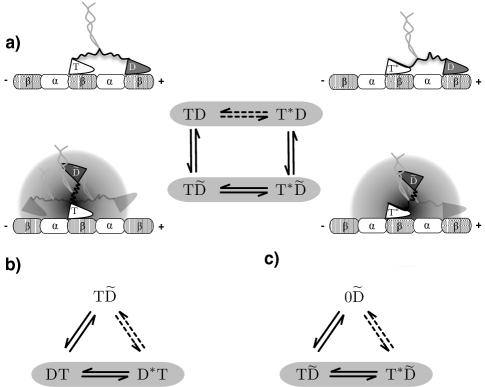
Figure 1:

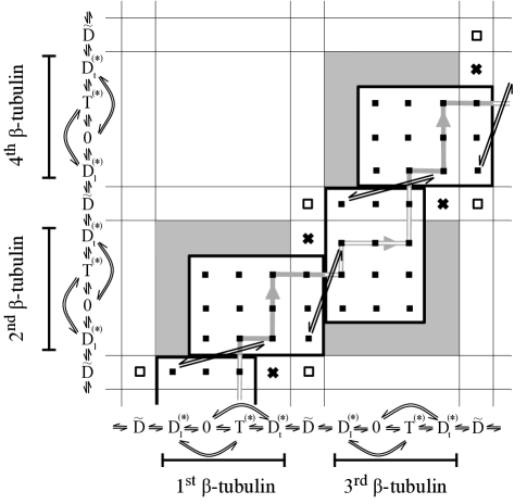
Figure 2:

Figure 3:

Figure 4:

Figure 5:

References

- (1) Rice, S., A. W. Lin, D. Safer, C. L. Hart, N. Naber, B. O. Carragher, S. M. Cain, E. Pechatnikova, E. M. Wilson-Kubalek, M. Whittaker, E. Pate, R. Cooke, E. W. Taylor, R. A. Milligan, and R. D. Vale. 1999. A structural change in the kinesin motor protein that drives motility. Nature. 402:778–784.
- (2) Vale, R. D., and R. A. Milligan. 2000. The way things move: looking under the hood of molecular motor proteins. Science. 288:88–95.
- (3) Hwang, W., M. J. Lang, and M. Karplus. 2008. Force generation in kinesin hinges on cover-neck bundle formation. Structure. 16:62–71.
- (4) Kikkawa, M. 2008. The role of microtubules in processive kinesin movement. Trends Cell Biol. 18:128–135.
- (5) Cross, R. A. 2004. The kinetic mechanism of kinesin. Trends Biochem. Sci. 29:301–309.
- (6) Block, S. M. 2007. Kinesin motor mechanics: binding, stepping, tracking, gating, and limping. Biophys. J. 92:2986–2995.
- (7) Mather, W. H., and R. F. Fox. 2006. Kinesin’s biased stepping mechanism: amplification of neck linker zippering. Biophys. J. 91:2416–2426.
- (8) Uemura, S., and S. Ishiwata. 2003. Loading direction regulates the affinity of ADP for kinesin. Nat. Struct. Biol. 10:308–311.
- (9) Rice, S., Y. Cui, C. Sindelar, N. Naber, M. Matuska, R. Vale, and R. Cooke. 2003. Thermodynamic properties of the kinesin neck-region docking to the catalytic core. Biophys. J. 84:1844–1854.
- (10) Visscher, K., M. J. Schnitzer, and S. M. Block. 1999. Single kinesin molecules studied with a molecular force clamp. Nature. 400:184–189.
- (11) Nishiyama, M., H. Higuchi, and T. Yanagida. 2002. Chemomechanical coupling of the forward and backward steps of single kinesin molecules. Nat. Cell Biol. 4:790–797.
- (12) Yildiz, A., M. Tomishige, R. D. Vale, and P. R. Selvin. 2004. Kinesin walks hand-over-hand. Science. 303:676–678.
- (13) Carter, N. J., and R. A. Cross. 2005. Mechanics of the kinesin step. Nature. 435:308–312.
- (14) Mori, T., R. D. Vale, and M. Tomishige. 2007. How kinesin waits between steps. Nature. 450:750–754.
- (15) Fehr, A. N., C. L. Asbury, and S. M. Block. 2008. Kinesin steps do not alternate in size. Biophys. J. 94:L20–L22.
- (16) Peskin, C. S., and G. Oster. 1995. Coordinated hydrolysis explains the mechanical behavior of kinesin. Biophys. J. 68:S202–S211.
- (17) Derényi, I., and T. Vicsek. 1996. The kinesin walk: a dynamic model with elastically coupled heads. Proc. Natl. Acad. Sci. USA. 93:6775–6779.
- (18) Liepelt, S., and R. Lipowsky. 2007. Kinesin’s network of chemomechanical motor cycles. Phys. Rev. Lett. 98:258102.
- (19) Vilfan, A. 2005. Elastic lever-arm model for myosin V. Biophys. J. 88:3792–3805.
- (20) Hyeon, C., and J. N. Onuchic. 2007. Internal strain regulates the nucleotide binding site of the kinesin leading head. Proc. Natl. Acad. Sci. USA. 104:2175–2180.
- (21) Ray, S., E. Meyhofer, R. A. Milligan, and J. Howard. 1993. Kinesin follows the microtubule’s protofilament axis. J. Cell Biol. 121:1083–1093.
- (22) Yildiz, A., M. Tomishige, A. Gennerich, and R. D. Vale. 2008. Intramolecular strain coordinates kinesin stepping behavior along microtubules. Cell. 134:1030–1041.
- (23) Asbury, C. L., A. N. Fehr, and S. M. Block. 2003. Kinesin moves by an asymmetric hand-over-hand mechanism. Science. 302:2130–2134.
- (24) Schief, W. R., R. H. Clark, A. H. Crevenna, and J. Howard. 2004. Inhibition of kinesin motility by ADP and phosphate supports a hand-over-hand mechanism. Proc. Natl. Acad. Sci. USA. 101:1183–1188.
- (25) Czövek, A., G. J. Szöllősi, and I. Derényi. 2008. The relevance of neck linker docking in the motility of kinesin. BioSystems. 93:29–33.
- (26) Schnitzer, M. J., and S. M. Block. 1997. Kinesin hydrolyses one ATP per 8-nm step. Nature. 388:386–390.
- (27) Vale, R. D., T. Funatsu, D. W. Pierce, L. Romberg, Y. Harada, and T. Yanagida. 1996. Direct observation of single kinesin molecules moving along microtubules. Nature. 380:451–453.
- (28) Yajima, J., M. C. Alonso, R. A. Cross, and Y. Y. Toyoshima. 2002. Direct long-term observation of kinesin processivity at low load. Curr. Biol. 12:301–306.
- (29) Visscher, K., M. J. Schnitzer, and S. M. Block. 1999. Single kinesin molecules studied with a molecular force clamp. Nature. 400:184–189.
- (30) Case, R. B., S. Rice, C. L. Hart, B. Ly, and R. D. Vale. 2000. Role of the kinesin neck linker and catalytic core in microtubule-based motility. Curr. Biol. 10:157–160.
- (31) Hackney, D. D. 1994. Evidence for alternating head catalysis by kinesin during microtubule-stimulated ATP hydrolysis. Proc. Natl. Acad. Sci. USA. 91:6865–6869.
- (32) Ma, Y. Z., and E. W. Taylor. 1995. Kinetic mechanism of kinesin motor domain. Biochemistry. 34:13233–13241.
- (33) Gilbert, S. P., and K. A. Johnson. 1994. Pre-steady-state kinetics of the microtubule-kinesin ATPase. Biochemistry. 33:1951–1960.
- (34) Gilbert, S. P., M. R. Webb, M. Brune, and K. A. Johnson. 1995. Pathway of processive ATP hydrolysis by kinesin. Nature. 373:671–676.
- (35) Farrell, C. M., A. T. Mackey, L. M. Klumpp, and S. P. Gilbert. 2002. The role of ATP hydrolysis for kinesin processivity. J. Biol. Chem. 277:17079–17087.
- (36) Auerbach, S. D., and K. A. Johnson. 2005. Alternating site ATPase pathway of rat conventional kinesin. J. Biol. Chem. 280:37048.
- (37) Ma, Y. Z., and E. W. Taylor. 1997a. Kinetic mechanism of a monomeric kinesin construct. J. Biol. Chem. 272:717–723.
- (38) Ma, Y. Z., and E. W. Taylor. 1997b. Interacting head mechanism of microtubule-kinesin ATPase. J. Biol. Chem. 272:724–730.
- (39) Rice, S., A. W. Lin, D. Safer, C. L. Hart, N. Naber, B. O. Carragher, S. M. Cain, E. Pechatnikova, E. M. Wilson-Kubalek, M. Whittaker, et al. 1999. A structural change in the kinesin motor protein that drives motility. Nature. 402:778–784.
- (40) Crevel, I. M. T. C., M. Nyitrai, M. C. Alonso, S. Weiss, M. A. Geeves, and R. A. Cross. 2004. What kinesin does at roadblocks: the coordination mechanism for molecular walking. EMBO J. 23:23–32.
- (41) Moyer, M. L., S. P. Gilbert, and K. A. Johnson. 1998. Pathway of ATP hydrolysis by monomeric and dimeric kinesin. Biochemistry. 37:800–813.