Anomalous scaling of passive scalars in rotating flows

Abstract

We present results of direct numerical simulations of passive scalar advection and diffusion in turbulent rotating flows. Scaling laws and the development of anisotropy are studied in spectral space, and in real space using an axisymmetric decomposition of velocity and passive scalar structure functions. The passive scalar is more anisotropic than the velocity field, and its power spectrum follows a spectral law consistent with $\sim k_{\perp}^{-3/2}$. This scaling is explained with phenomenological arguments that consider the effect of rotation. Intermittency is characterized using scaling exponents and probability density functions of velocity and passive scalar increments. In the presence of rotation, intermittency in the velocity field decreases more noticeably than in the passive scalar. The scaling exponents show good agreement with Kraichnan’s prediction for passive scalar intermittency in two-dimensions, after correcting for the observed scaling of the second order exponent.

I Introduction

A passive scalar is a quantity diluted in a fluid in such a low concentration that it does not affect the flow evolution, but that it is advected and diffused by the flow. Examples are given by colorant dye used in experiments, and aerosols and pollutants in small concentrations in the atmosphere. In recent years, the study of passive scalars has been associated with substantial advances in our theoretical understanding of turbulent flows Kraichnan (1994); Chen and Kraichnan (1998); Falkovich et al. (2001). Passive scalars share similarities with three dimensional hydrodynamic turbulence, developing a direct cascade (a transfer of variance towards smaller scales with constant flux), and intermittency (the spontaneous development of strong gradients at small scales). As in the study of Navier-Stokes turbulence, some topics of interest include the persistence of anisotropy at small scales Sreenivasan (1991); Warhaft (2000), universality, and deviations from scale-invariance associated with intermittent events. For the passive scalar, significant advances to understand these topics have been made in the framework of the Kraichnan model Kraichnan (1968, 1994); Chertkov et al. (1996). For a random delta-correlated in time velocity field, the scaling exponents of the passive scalar were obtained and shown to have anomalous (intermittent) behavior but to be universal. Numerical simulations and experiments showed good agreement with these results Chen and Kraichnan (1998). The results were later also extended to consider the behavior of probability density functions, or differences between passive and active scalars (see, e.g., Celani et al. (2004)).

Passive scalars in rotating turbulence have received less attention. It is well known that one of the effects of rotation is to modify the energy transfer, transferring the energy preferentially towards modes perpendicular to the rotation axis Cambon and Jacquin (1989); Waleffe (1992); Cambon et al. (1997). This results in a two-dimensionalization of the flow, and in the development of an inverse energy cascade. High resolution simulations agree with these results, and also indicate that intermittency in the velocity field is substantially reduced by rotation Müller and Thiele (2007); Mininni and Pouquet (2009); Mininni and Pouquet (2010a, b). Passive scalar transport has been studied in numerical simulations showing that its transfer is affected by rotation Yeung and Xu (2004); Brethouwer (2005), and in experiments Moisy et al. (2001) showing that passive scalars in rotating flows still develop anomalous scaling in their structure functions.

In this paper we analyze data from direct numerical simulations of the Navier-Stokes equation in a rotating frame, together with the advection-diffusion equation for the passive scalar. Spatial resolution is $512^{3}$ grid points in a regular periodic grid. Passive scalar is injected into an initially homogeneous and isotropic turbulent flow, sustained by an external (random) mechanical force. After reaching a steady state, rotation is turned on. Two different scales are considered for the injection of mechanical energy and passive scalar. In one case, both are injected at the largest available scale in the domain. In the other, both are injected at an intermediate scale, to allow the mechanical energy develop some inverse transfer and to see whether this transfer affects the intermittency of the passive scalar. Two different rotation rates are considered, in both cases chosen to study the regime of moderate Rossby numbers. Inertial range scaling is studied considering the energy and passive scalar spectra and fluxes. Velocity and passive scalar structure functions are computed using an axisymmetric decomposition, and the corresponding scaling exponents are considered to characterize intermittency in each field. Finally, probability density functions of increments of the velocity and the passive scalar are studied, together with visualizations of the fields. We find that the passive scalar is more anisotropic than the velocity field at small scales, and follows a spectral law consistent with $\sim k_{\perp}^{-3/2}$, where $k_{\perp}$ denotes wave vectors perpendicular to the rotation axis. While intermittency in the velocity field is strongly decreased in the rotating case, the passive scalar is still intermittent and its scaling exponents show good agreement with Kraichnan’s prediction for passive scalar intermittency in two-dimensions.

II Setup and theory

II.1 Basic equations, code, and simulations

For an incompressible fluid with uniform mass density in a rotating frame, the Navier-Stokes equation for the velocity field ${\bf u}$, and the equation for the passive scalar ${\theta}$ are,

$$\partial_{t}{\bf u}+{\bf u}\cdot\nabla{\bf u}=-2{\bf\Omega}\times{\bf u}-\nabla p+\nu\nabla^{2}{\bf u}+{\bf f},$$ (1)

$$\nabla\cdot{\bf u}=0,$$ (2)

$$\partial_{t}{\theta}+{\bf u}\cdot\nabla{\theta}=\kappa\nabla^{2}{\theta}+{\bf\phi},$$ (3)

where $p$ is the pressure divided by the mass density, $\nu$ is the kinematic viscosity, and $\kappa$ is the scalar diffusivity. Here, ${\bf f}$ is an external force that drives the turbulence, ${\phi}$ is the source of the scalar field, and ${\bf\Omega}=\Omega\hat{z}$ is the rotation angular velocity.

For the analysis in the following sections we use data stemming from direct numerical simulations of the above equations. We solve Eqs. (1), (2) and (3) using a parallel pseudospectral code in a three dimensional domain of size $2\pi$ with periodic boundary conditions Gómez et al. (2005a, b). The pressure is obtained by taking the divergence of Eq. (1), using the incompressibility condition (2), and solving the resulting Poisson equation. The equations are evolved in time using a second order Runge-Kutta method. The code uses the $2/3$-rule for dealiasing, and as a result the maximum wave number is $k_{max}=N/3$, where $N$ is the number of grid points in each direction. All simulations presented are well resolved, in the sense that the dissipation wave numbers $k_{\nu}$ and $k_{\kappa}$ are smaller than the maximum wave number $k_{max}$ at all times.

The practice of numerically solving flows in a rotating frame in periodic boxes dates back to Ref. Bardina et al. (1985). Basically, strict periodicity in all three spatial directions replaces the hypothesis of homogeneity. With these boundary conditions, the centrifugal force (not written in Eq. 1) can be written as a gradient and absorved into the pressure, and is thus automatically taken into account when the Poisson equation is solved. The rotating flow is thus considered infinite, homogeneous, with constant rotation rate $\Omega$, and locally expanded in the rotating frame using a Fourier series (in the same way local instabilities are studied in unbounded flows). There are however two differences between an infinite and a periodic flow. A periodic flow is bounded in the sense that eddies larger than the size of the box ($2\pi$ in our dimensionless units) cannot develop. This will be important when we consider separation of scales in the inverse energy cascade. Also, there is a discussion concerning whether decoupling between two-dimensional modes and fast waves takes place in rotating flows. While first-order decoupling was shown for periodic flows (which have discrete wave numbers) Babin et al. (1996), for infinite domains with continuous wave numbers decoupling does not hold Cambon et al. (2004). In practice, both idealizations have limitations, as other effects in bounded flows (e.g., Ekman layers) are not present with these boundary conditions.

The runs are characterized by Reynolds, Peclet, and Rossby numbers. The Reynolds, Schmidt, and Peclet numbers are defined as usual as

$$R_{e}=\frac{UL}{\nu},$$ (4)

$$S_{c}=\frac{\nu}{\kappa},$$ (5)

$$P_{e}=S_{c}R_{e},$$ (6)

where $U$ is the r.m.s.velocity, and $L$ is the forcing scale of the flow defined as $2\pi/k_{F}$, with $k_{F}$ the forcing wave number (when the forcing is applied in a wide band of wave numbers, $k_{F}$ is taken as the minimum of the wave numbers in the band). For the simulations, $U\approx 1$, and all runs have $\nu=\kappa$ (i.e., $S_{c}=1$ and $P_{e}=R_{e}$).

To characterize the strength of rotation, we use the Rossby number

$$R_{o}=\frac{U}{2L\Omega}.$$ (7)

It is also useful to introduce a micro-Rossby number defined as the ratio of the r.m.s. vorticity $\omega_{\textrm{rms}}$ (${\bf\omega}=\nabla\times{\bf u}$) to the background vorticity,

$$R_{\omega}=\frac{\omega_{\textrm{rms}}}{2\Omega}.$$ (8)

For rotation to be important, the Rossby number $R_{o}$ should be smaller than one, but the micro-Rossby number $R_{\omega}$ should be close to one or larger. If $R_{\omega}$ is much smaller than one, non-linear interactions are rapidly damped by the scrambling effect of Rossby waves, resulting in a strong quenching of turbulence by rotation Cambon et al. (1997).

Several simulations were done with fixed linear spatial resolution ($N=512$), and same kinematic viscosity ($\nu=\kappa=6\times 10^{-4}$). Parameters for all runs are given in Table 1. The forcing used for the velocity field as well as for the passive scalar is a superposition of Fourier modes with random phases, delta-correlated in time, and injected at the same wave number $k_{F}$ for both fields. One set of runs (set A) has forcing applied at $k\in[1,2]$ (therefore $k_{F}=1$, and the simulations have the largest possible separation of scales in the direct energy cascade), while another set has forcing at $k=k_{F}=3$ (set B). This latter choice for the injection wave number leaves some room in spectral space for an inverse cascade of energy to develop, but also reduces the Reynolds number by a factor of three, as scale separation between injection and dissipation is smaller. This results in narrower inertial ranges for all simulations in set B. However, the scale separation between the box size and the forcing scale will allow us to compare runs with and without inverse energy transfer (respectively, sets B and A), and to see whether this transfer has some effect in the scaling of the passive scalar.

The procedure followed in the simulations in both sets was the same. A simulation of the Navier-Stokes equation with $\Omega=0$ was done first, until reaching an isotropic and homogeneous turbulent steady state (this takes approximately ten turnover times). Then, the passive scalar was injected, and the run was continued for other ten turnover times until reaching a steady state for the passive scalar (these runs correspond to run A1 of set A, and run B1 of set B). Finally, rotation was turned on. Different values of $\Omega$ were considered, to have similar Rossby numbers in both sets. These runs were started from the last snapshot of the velocity and the passive scalar of run A1 or B1. Each of these runs was continued for over twenty turnover times. Rossby numbers for each run are listed in Table 1.

Table 1: Parameters used in the simulations. $k_{F}$ is the forcing wave number, $\Omega$ the rotation, $R_{o}$ the Rossby number $R_{e}$ the Reynolds number, and $R_{\omega}$ the micro-Rossby number.

Run	$k_{F}$	$\Omega$	$R_{o}$	$R_{e}$	$R_{\omega}$
A1	1	0	$\infty$	1000	$\infty$
A2	1	4	$0.04$	1000	$0.9$
B1	3	0	$\infty$	240	$\infty$
B2	3	12	$0.04$	240	$0.4$

II.2 Analysis

Characterization of the flow and passive scalar anisotropy, scaling laws, and intermittency is done considering power spectra, fluxes, structure functions, and probability density functions of field increments.

Isotropic energy spectrum and power spectrum of the scalar field are defined as usual (summing the power of all modes in Fourier space over spherical shells), and denoted by $E(k)$ and $V(k)$ respectively. Since rotation introduces a preferred direction, anisotropies will be characterized in spectral space using the so-called reduced spectra. The reduced perpendicular energy spectrum $E(k_{\perp})$ and scalar power spectrum $V(k_{\perp})$ result from summing the power of all modes in cylindrical shells of radius $k_{\perp}$, with their axis aligned with the rotation axis $\hat{z}$. The reduced parallel spectra $E(k_{\parallel})$ and $V(k_{\parallel})$ result from summing the power of all modes in planes with $k_{z}=k_{\parallel}$. Detailed definitions can be found in Mininni and Pouquet (2009).

Two-dimensional axisymmetric spectra can be also defined (see e.g., Cambon et al. (1997)), and give more detailed information of spectral anisotropy. Instead, we will consider here an axisymmetric decomposition of structure functions, which will also give us information of intermittency in the velocity and scalar fields. Longitudinal increments of the velocity and passive scalar fields are defined as:

$$\delta u({\bf x},{\bf l})=\left[{\bf u}({\bf x}+{\bf l})-{\bf u}({\bf x})\right]\cdot\frac{{\bf l}}{|{\bf l}|},$$ (9)

$$\delta\theta({\bf x},{\bf l})=\left[\theta({\bf x}+{\bf l})-\theta({\bf x})\right]\cdot\frac{{\bf l}}{|{\bf l}|},$$ (10)

where the increment ${\bf l}$ can point in any direction. Structure functions of order $p$ are then defined as

$$S_{p}({\bf l})=\left\langle\delta u^{p}({\bf x},{\bf l})\right\rangle,$$ (11)

for the velocity field, and as

$$T_{p}({\bf l})=\left\langle\delta\theta^{p}({\bf x},{\bf l})\right\rangle,$$ (12)

for the passive scalar field. Here, brackets denote spacial average over all values of ${\bf x}$.

These structure functions depend on the direction of the increment. In simulations without rotation, the field is isotropic and the $SO(3)$ decomposition was used to calculate the isotropic component of these structure functions Arad et al. (1998); Biferale and Vergassola (2001); Biferale and Procaccia (2005); Martin and Mininni (2010). The decomposition was implemented computing (and averaging) the structure functions for 146 different directions that cover almost isotropically the sphere, using the method described in Taylor et al. (2003). In runs with rotation, given the preferred direction and the axisymmetry associated with it, we will be interested in increments parallel and perpendicular to ${\bf\Omega}$. We denote increments in these two directions as $l_{\parallel}$ and $l_{\perp}$ respectively. We then follow the procedure explained in Mininni and Pouquet (2010b) to perform a decomposition of structure functions based on the $SO(2)\times\Re$ symmetry group (rotations in the $xy$ plane plus translations in the $z$ direction). Velocity and passive scalar structure functions were computed using 26 different directions for the increments ${\bf l}$, generated by integer multiples of the vectors $(1,0,0)$, $(1,1,0)$, $(2,1,0)$, $(3,1,0)$, $(0,1,0)$, $(-1,1,0)$, $(1,2,0)$, $(-2,1,0)$, $(-1,2,0)$, $(1,3,0)$, $(-3,1,0)$, $(-1,3,0)$, and $(0,0,1)$ for translations in $z$ (all vectors are in units of grid points in the simulations), plus the 13 vectors obtained by multiplying them by $-1$. Once these structure functions were calculated, the perpendicular structure functions $S_{p}(l_{\perp})$ and $T_{p}(l_{\perp})$ were obtained by averaging over the $24$ directions in the $xy$ plane, and the parallel structure functions $S_{p}(l_{\parallel})$ and $T_{p}(l_{\parallel})$ were computed directly using the generators in the $z$ direction.

For runs in set A, this procedure was applied to eight snapshots of the velocity and passive scalar fields separated by at least one turnover time each, while for runs in set B we analyzed six snapshots. For large enough Reynolds number, the structure functions are expected to show inertial range scaling, i.e., we expect that for some range of scales $S_{p}\sim l^{\xi_{p}}$ and $T_{p}\sim l^{\zeta_{p}}$ ($l$ may be replaced by $l_{\perp}$ or $l_{\parallel}$ in the rotating case), where $\xi_{p}$ and $\zeta_{p}$ are, respectively, the scaling exponents of order $p$ of the velocity and scalar fields. Scaling exponents shown in the following sections are calculated for all the snapshots analyzed in each simulation, and averaged over time. Errors are then defined as the mean square error; e.g., for the passive scalar exponents, the error is

$$e_{\zeta_{p}}=\frac{1}{N}\sqrt{\sum_{i=1}^{N}\left(\zeta_{p_{i}}-\overline{\zeta_{p}}\right)^{2}},$$ (13)

where $N$ is the number of snapshots of the field, $\zeta_{p_{i}}$ is the slope obtained from a least square fit for the $i$-th snapshot, and $\overline{\zeta_{p}}$ is the mean value averaged over all snapshots. The error in the least square calculation of the slope for each snapshot is much smaller than this mean square error. Extended self-similarity Benzi et al. (1993a, b) is not used to obtain the scaling exponents.

III Numerical Results

III.1 Spectra and fluxes

In the absence of rotation, velocity and passive scalar spectra follow a similar inertial range scaling, close to $\sim k^{-5/3}$ as expected from Kolmogorov phenomenology, except for bottleneck and possible intermittency corrections (the latter only visible in the spectrum at higher resolution Ishida et al. (2006); Yeung et al. (2005)). As an example, Figure 1 shows the energy and passive scalar spectra for run A1 in the turbulent steady state. The slope indicates a $\sim k^{-5/3}$ scaling law.

Figure 1: Energy (solid) and passive scalar (dash-dotted) spectrum for run A1. Kolmogorov scaling is shown as a reference.

Once rotation is turned on, the spectral scaling of the passive scalar and velocity changes. Figure 2(a) shows the reduced perpendicular energy spectrum $E(k_{\perp})$ for run A2, together with the reduced perpendicular passive scalar power spectrum $V(k_{\perp})$. The spectral scaling of the velocity field changes and gets closer to the expected $E(k_{\perp})\sim k_{\perp}^{-2}$ Zhou (1995); Müller and Thiele (2007), while the passive scalar is close to $\sim k_{\perp}^{-3/2}$ scaling. This can be further confirmed in the compensated spectra shown in 2(b).

Figure 2: (a) Energy (solid) and passive scalar (dash-dotted) reduced perpendicular spectrum for run A2. Slopes are shown as a reference. (b) Reduced perpendicular energy spectrum compensated by $k_{\perp}^{-2}$, and passive scalar power spectrum compensated by $k_{\perp}^{-3/2}$ for the same run.

Figure 3 shows the reduced perpendicular energy and passive scalar spectra for run B2; $E(k_{\perp})$ is also close to $\sim k_{\perp}^{-2}$, and $V(k_{\perp})$ again is close to $k_{\perp}^{-3/2}$. Note run B2 is forced at $k_{F}=3$, and as already mentioned, in the presence of rotation there is some room in spectral space for inverse transfer of energy towards larger scales (indeed, at much later times the energy spectrum in this run peaks at $k=1$). However, the scaling of the passive scalar seems to be insensitive to the development of such an inverse energy transfer. Since both sets of runs show similar scaling, in the following we will concentrate on runs in set A (which have a larger scale separation between injection and dissipation, and therefore a better resolved direct cascade range), and only resort to runs in set B for comparisons.

Unlike the scaling laws observed in the reduced perpendicular spectra of runs with rotation, isotropic and reduced parallel spectra show less clear behavior. Figure 4(a) shows the isotropic energy and passive scalar spectra for run A2. The isotropic energy spectrum shows a scaling law similar to $k^{-2}$. However, the isotropic passive scalar power spectrum shows a steeper spectrum with no clear inertial range, hinting at a more anisotropic spectral distribution than the energy at scales smaller than the forcing scale. In the case of the reduced parallel spectra, no clear power law can be identified for $E(k_{\parallel})$ and $V(k_{\parallel})$; see Fig. 4(b).

Several quantities can be used to measure the development of anisotropies in a rotating flow Cambon and Jacquin (1989); Bartello et al. (1994); Cambon et al. (1997). As an example, the ratio of energy in all modes with $k_{\parallel}=0$ to the total energy, i.e., $E(k_{\parallel}=0)/E$, can be used to characterize large scale anisotropy Mininni and Pouquet (2009). For a purely two-dimensional flow, this ratio is equal to one. For the passive scalar, the equivalent quantity $V(k_{\parallel}=0)/V$ can also be used. In the simulations without rotation, the mean values of $E(k_{\parallel}=0)/E$ and $V(k_{\parallel}=0)/V$ are close to $0.1$. As can be seen in Table 2, these ratios increase when rotation is turned on, with $E(k_{\parallel}=0)/E$ larger than $V(k_{\parallel}=0)/V$ in all cases. This suggests that, at large scales, the velocity field is more anisotropic than the passive scalar field.

To quantify small-scale anisotropy, the Shebalin angles can be used instead. These were originally introduced to study anisotropy in magnetohydrodynamic turbulence Shebalin et al. (1983); Milano et al. (2001), and for the velocity are given by

$$\tan^{2}(\alpha_{u})=2\lim_{l\to 0}\frac{S_{2}(l_{\perp})}{S_{2}(l_{\parallel})}=2\dfrac{\sum_{k_{\perp}}k_{\perp}^{2}E(k_{\perp})}{\sum_{k_{\parallel}}k_{\parallel}^{2}E(k_{\parallel})}.$$ (14)

The angle $\alpha_{u}$ gives a global measure of small-scale anisotropy, with a value of $\tan^{2}(\alpha_{u})=2$ corresponding to an isotropic flow. The square tangent of the Shebalin angles for the velocity and passive scalar fields, respectively, $\tan^{2}(\alpha_{u})$ and $\tan^{2}(\alpha_{\theta})$, are given in Table 2 for runs with rotation. The values of $\tan^{2}(\alpha_{\theta})$ are larger than the values of $\tan^{2}(\alpha_{u})$, indicating that the passive scalar field is more anisotropic than the velocity field in the small scales. This slower recovery of small-scale isotropy by the passive scalar, when compared with the velocity field, has already been reported in the case of non-rotating turbulence, see e.g., Warhaft (2000), but not in the rotating case to the best of our knowledge.

Table 2: Anisotropy in runs with rotation. $E(k_{\parallel}=0)/E$ is the ratio of energy in all modes with $k_{\parallel}=0$ to the total energy, $V(k_{\parallel}=0)/V$ is the ratio of scalar variance in all modes with $k_{\parallel}=0$ to the total scalar variance, $\tan^{2}(\alpha_{u})$ is the square tangent of the Shebalin angle for the velocity field, and $\tan^{2}(\alpha_{\theta})$ is the square tangent of the Shebalin angle for the passive scalar.

Run	$E(k_{\parallel}=0)/E$	$V(k_{\parallel}=0)/V$	$\tan^{2}(\alpha_{u})$	$\tan^{2}(\alpha_{\theta})$
A2	0.5	0.4	13	20
B2	0.2	0.1	14	50

The growth of energy at $k=1$, and the flux of energy towards large scales, associated with the two-dimensionalization of the flow resulting from rotation, can only be observed in run B2 (see Fig. 5). As mentioned before, this run has some room in spectral space between the largest wave number in the box and the forcing wave number. Figure 5 shows the energy and passive scalar fluxes in runs B1 and B2 (without and with rotation, respectively) as a comparison. In the absence of rotation, the energy flux shows a direct cascade range (a range of positive and approximately constant flux), while the energy flux is negligible for wave numbers smaller than the forcing wave number ($k\leq k_{F}$). The passive scalar flux shows a similar behavior. In the presence of rotation, the energy flux becomes negative for $k\leq k_{F}$, indicating energy is transferred towards scales larger than the forcing scale, and the flux towards smaller scales decreases. Scale separation is too small to talk of an inverse cascade of energy with constant flux, but computational limitations in our attempt to have a well resolved direct cascade of passive scalar limits our ability to resolve an inverse energy cascade. For the passive scalar, no flux toward larger scales is observed, and the amplitude of the positive (direct) flux decreases by a small fraction.

Based on these results, we can put forward a phenomenological argument considering the effect of rotation, to obtain the inertial range spectrum of passive scalar observed in the simulations. From Eq. (3), we can estimate the flux of passive scalar as

$$\sigma\sim\frac{u_{l_{\perp}}\theta_{l_{\perp}}^{2}}{l_{\perp}},$$ (15)

where $u_{l_{\perp}}$ is the characteristic velocity at the scale $l_{\perp}$, and $\theta_{l_{\perp}}$ is the characteristic concentration of passive scalar at the same scale. Using that the passive scalar flux is constant in the inertial range, then $\theta_{l_{\perp}}$ scales as $\theta_{l_{\perp}}^{2}\sim\sigma l_{\perp}/u_{l_{\perp}}$. If the energy spectrum in the direct energy cascade range follows a power law $E(k_{\perp})\sim k_{\perp}^{-2}$, then in the absence of intermittency corrections $u_{l_{\perp}}\sim l_{\perp}^{1/2}$, and

$$V(k_{\perp})\sim\sigma k_{\perp}^{-3/2}.$$ (16)

Figure 3: (a) Reduced perpendicular energy (solid) and passive scalar (dash-dotted) spectra for run B2. (b) Reduced perpendicular energy spectrum compensated by $k_{\perp}^{-2}$ and reduced perpendicular passive scalar power spectrum compensated by $k_{\perp}^{-3/2}$.

Figure 4: (a) Isotropic energy (solid) and passive scalar (dash-dotted) spectra for run A2. (b) Reduced parallel energy (solid) and passive scalar (dash-dotted) spectra for the same run.

Figure 5: (a) Energy flux $\Pi(k)$ (solid) and passive scalar flux $\sigma(k)$ (dash-dotted) for run B1. (b) Same for run B2.

III.2 Structure functions and scaling exponents

We now consider isotropic and axisymmetric velocity and passive scalar structure functions for the simulations described above, using the method explained in Sec. II.2.

Figure 6(a) shows the result of computing the passive scalar structure functions in run A1 (isotropic) and A2 (axisymmetric, only structure functions with $l_{\perp}$ increments are shown), for one instantaneous snapshot of the scalar field (at $t=7$ in run A1, and at $t=18$ in run A2). The structure functions show a range of scales with approximately power law scaling at intermediate scales, and at the smallest scales approach the $\sim l^{p}$ scaling expected for a smooth field in the dissipative range.

Figure 6: (a) Isotropic structure functions for the passive scalar up to 8th order in run A1, at $t=7$. (b) Axisymmetric (only for $l_{\perp}$ increments) structure functions for the passive scalar up to 8th order in run A2, at $t=18$.

Figure 7 shows a detail for rotating runs A2 and B2 of the passive scalar second order axisymmetric structure functions in the perpendicular direction $T_{2}(l_{\perp})$ (i.e., averaged in all directions in the $xy$ plane), and in the parallel direction, $T_{2}(l_{\parallel})$. Stronger anisotropy is observed at small scales, manifested as a different (steeper) dependence of $T_{2}(l_{\parallel})$ with the spatial increment when compared with $T_{2}(l_{\perp})$, and as a much smaller amplitude of $T_{2}(l_{\parallel})$ at small scales.

An inertial range with power law-scaling can be identified at intermediate scales in $T_{2}(l_{\perp})$, but not so clearly in $T_{2}(l_{\parallel})$ (this is specially true for run B2, where the parallel structure function shows only the smooth scaling $~{}l_{\parallel}^{2}$). This is consistent with results shown in the previous section for the reduced passive scalar spectra. Inertial range with power-law scaling was observed for the reduced perpendicular spectrum $V(k_{\perp})$, while no clear scaling could be identified for $V(k_{\parallel})$. Note also that at scales close to the forcing scale or larger, the passive scalar distribution always seems to be more isotropic, in agreement with the results shown in Table 2.

The slopes indicated as a reference in Fig. 7 correspond to the time average of the second order scaling exponent, obtained from a best fit in the inertial range of all structure functions at different times available for each run (eight snapshots for run A2, and six snapshots for run B2). The second order scaling exponents (in the perpendicular direction) for the passive scalar thus obtained are $\zeta_{2}\approx 0.49\pm 0.01$ in run A2, and $\zeta_{2}\approx 0.50\pm 0.01$ in run B2.

Figure 7: Axisymmetric second order structure functions for the passive scalar: (a) run A2 with $\Omega=4$ at $t=18$, and (b) run B2 with $\Omega=12$ at $t=14$. $T_{2}(l_{\perp})$ corresponds to dashed lines and $T_{2}(l_{\parallel})$ to full lines. Slopes indicated as references correspond to the time average of the scaling exponents, obtained from a best fit in the inertial range of the structure functions at different times.

The values obtained for $\zeta_{2}$ are in good agreement with the $V(k_{\perp})\sim k_{\perp}^{-3/2}$ power law found for the reduced perpendicular passive scalar spectrum, which leads on dimensional grounds to $T_{2}(l_{\perp})\sim l_{\perp}^{-1/2}$.

Figure 8 shows the axisymmetric second order structure functions for the velocity field, for runs with rotation at late times. Small-scale anisotropy develops, and is more clearly seen in run B2 with $\Omega=12$. At large scales, stronger correlations are observed in the parallel direction in this latter case, which is to be expected as this simulation has some separation between the largest scale available in the box and the forcing scale, and the flow becomes quasi-2D at large scales. Comparing these structure functions with the ones for the passive scalar in Fig. 7, it becomes apparent that at the Rossby number considered, the small-scale anisotropy associated with rotation is stronger for the passive scalar than for the velocity field.

Inertial range with power law scaling is also observed for velocity structure functions. For runs A2 and B2, time averaged second order scaling exponents, corresponding to scaling $S_{2}(l_{\perp})\sim l_{\perp}^{\xi_{2}}$, are indicated as a reference by the slopes in Figs. 8(a) and  8(b). Second order scaling exponents are $\xi_{2}\approx 0.96\pm 0.01$ for run A2, and $\xi_{2}\approx 0.98\pm 0.01$ for run B2. These values are consistent with the inertial range scaling found for the perpendicular energy spectrum in these runs, $E(k_{\perp})\sim k_{\perp}^{-2}$, which leads to $S_{2}(l_{\perp})\sim l_{\perp}^{-1}$.

Figure 8: Axisymmetric second order structure functions for the velocity field: (a) run A2 with $\Omega=4$ at $t=18$, and (b) run B2 with $\Omega=12$ at $t=14$. $S_{2}(l_{\perp})$ corresponds to dashed lines and $S_{2}(l_{\parallel})$ to full lines. Slopes indicated as references correspond to the time average of the scaling exponents, obtained from a best fit in the inertial range of all structure functions at different times.

From the curves in Fig. 6, scaling exponents can be computed for higher orders. Velocity and passive scalar exponents in the direct cascade range were computed for runs in set A up to the seventh order. For runs in set B, scaling exponents were only computed up to the sixth order, as those runs have smaller scale separation between forcing and dissipation.

Figure 9 shows the velocity and scalar exponents for runs A1 and B1 (no rotation). For the velocity field, exponents in both runs are similar. The third order velocity field exponent is $\xi_{3}=0.99\pm 0.02$ for run A1, and $\xi_{3}=0.98\pm 0.01$ for run B1, in good agreement with the value of $1$ expected from the $4/5$-law for isotropic and homogeneous turbulence. The velocity field exponents display the well known deviations from the linear ($\xi_{p}=p/3$) Kolmogorov scaling associated with intermittency. This deviation from strict scale invariance is often quantified in terms of the intermittency exponent $\mu=2\xi_{3}-\xi_{6}$, which for these runs is $\mu=0.24\pm 0.12$ for run A1, and $\mu=0.25\pm 0.06$ for run B1. The higher order velocity exponents obtained from these runs are also consistent with previous results for non-rotating turbulence at large Reynolds numbers Sreenivasan and Antonia (1997); She and Lévêque (1994); Martin and Mininni (2010).

The passive scalar exponents for these two runs also display similar values, which are consistent (within error bars) with the values of the velocity field exponents for orders $p=1$ and 2, and show larger deviations from the Kolmogorov scale invariant prediction for larger values of $p$. This is a well known result which indicates that the passive scalar in isotropic and homogeneous turbulence is more intermittent than the velocity field Kraichnan (1994); Chertkov et al. (1996). For advection and diffusion of a passive scalar in a random, delta-correlated in time velocity field in a space with dimensionality $d$, Kraichnan obtained an expression for the passive scalar scaling exponents of all orders as a function of the second order exponent $\zeta_{2}$ Kraichnan (1994),

$$\zeta_{p}=\frac{1}{2}\left[\sqrt{2d\zeta_{2}p+(d-\zeta_{2})^{2}}+(d-\zeta_{2})\right].$$ (17)

This prediction is also shown in Fig. 9, with the exponents computed using the value of $\zeta_{2}$ obtained from the simulations, and for $d=3$. Deviations from this model, which start at $p=4$, are small when compared with the deviations of the data from the linear scaling. Similar deviations were also already reported in previous numerical simulations of passive scalar transport in turbulent flows Chen and Kraichnan (1998).

Figure 9: Scaling exponents (with error bars) as a function of the order $p$, for the velocity (stars for run A1 and diamonds for run B1), and the passive scalar (squares for run A1 and triangles for run B1). The solid line corresponds to Kolmogorov scaling $\xi_{p}=p/3$, and the dashed line corresponds to Kraichnan’s linear ansatz with $d=3$ and $\zeta_{2}=0.62$.

In the presence of rotation and for small Rossby number, velocity scaling exponents of a strictly self-similar flow are expected to follow a linear law $\xi_{p}=p/2$, if the energy spectrum scales as $\sim k_{\perp}^{-2}$. For runs A2 and B2, velocity scaling exponents are closer to the $p/2$ linear scaling, and display significantly smaller deviations from the straight line for the higher order exponents than in the non-rotating case (see Fig. 10). Velocity scaling exponents are similar for both runs with rotation. The intermittency coefficient in runs A2 and B2 is $\mu=0.1\pm 0.1$. As reported before Baraud et al. (2003); Müller and Thiele (2007); Seiwert et al. (2008); Mininni and Pouquet (2009); Mininni and Pouquet (2010b), for large enough rotation intermittency is substantially decreased.

Figure 10: Scaling exponents (with error bars) as a function of the order $p$, for the velocity (stars for run A2 and diamonds for run B2) and passive scalar (squares for run A2 and triangles for run B2). The solid line corresponds to linear scaling $\xi_{p}=p/2$, the dash-dotted line corresponds to linear scaling $\zeta_{p}=p/4$, and the dotted and dashed lines correspond respectively to the linear ansatz with $d=2$ and $d=3$ using $\zeta_{2}=0.5$.

Figure 10 also shows the scaling exponents for the passive scalar in runs with rotation. In the scale invariant (non-intermittent) case, a $\zeta_{p}=p/4$ linear law is expected for passive scalar exponents, if the second order exponent is $\zeta_{2}=1/2$. Deviations from this linear scaling are clearly visible in all runs (see, e.g, Fig. 10). For runs A2 and B2, Kraichnan’s linear ansatz (17) adjusts very accurately the numerical data with $\zeta_{2}=0.5$ and $d=2$. The good agreement with the model with $d=2$ for runs with small Rossby number again points to a strong bi-dimensionalization of the passive scalar distribution in the presence of rotation.

Intermittency of the passive scalar decreases with the Rossby number, although less than for velocity. The intermittency coefficient for the passive scalar, $\mu_{s}=2\zeta_{3}-\zeta_{6}$, is $\mu_{s}=0.4\pm 0.1$ for runs A1 and B1 ($\Omega=0$), and $\mu_{s}=0.2\pm 0.1$ and $\mu_{s}=0.22\pm 0.09$ for runs A2 and B2 respectively ($\Omega\neq 0$).

III.3 Probability density functions

Figure 11: Probability density functions for passive scalar and velocity increments in run A1, for five different spatial increments $l=1.6$ (solid), $0.8$ (dashed), $0.4$ (dashed-dotted), $0.2$ (dashed-dotted-dotted), and $0.1$ (long dashes). (a) Passive scalar, and (b) $x$-component of the velocity field. In both cases the dotted curve represents a Gaussian distribution with unit variance. Smaller increments have stronger non-Gaussian tails.

Figure 12: Probability density functions for passive scalar and velocity increments in run A2, for five different spatial increments $l=1.6$ (solid), $0.8$ (dashed), $0.4$ (dashed-dotted), $0.2$ (dashed-dotted-dotted), and $0.1$ (long dashes). (a) Passive scalar, and (b) $x$-component of the velocity field. A Gaussian curve with unit variance is indicated by the dotted curve. Again, as intervals are decreased, curves depart more and more from the Gaussian distribution.

In this section we consider probability density functions (PDFs) for longitudinal increments and derivatives of the $x$-component of the velocity field, as well as for the passive scalar. In all cases, curves shown are normalized by their variance, and a Gaussian curve with unit variance is shown as a reference. In a scale invariant flow the PDFs of the velocity and scalar increments are expected to be Gaussian and to collapse to a single curve when properly normalized. On the other hand, in an intermittent flow, probability density functions are expected to have strong non-Gaussian tails with larger amplitude as smaller spatial increments are considered. These tails are associated with the larger-than-Gaussian probability of extreme events to occur, which is the signature of intermittency.

Figure 11 shows the PDFs of the velocity and the passive scalar increments for four different values of the spatial increment $l=1.6$, $0.8$, $0.4$, $0.2$, and $0.1$, for run A1 ($\Omega=0$). As a reference, the forcing scale in this runs is $\approx 2\pi$ and the dissipative scale is $\approx 0.05$; $l=0.8$ and $0.4$ clearly correspond to scales in the inertial range. The PDFs of velocity and passive scalar increments for $l=1.6$ are close to Gaussian, while for smaller spatial increments non-Gaussian tails develop.

Figure 13: Probability density functions for velocity and passive scalar derivatives in the $x$ direction for run A1. (a) Passive scalar, and (b) $x$-component of the velocity field. Dotted curves represent a Gaussian distribution with unit variance.

Figure 14: Probability density functions for velocity and passive scalar derivatives in the $x$ direction for run A2. (a) Passive scalar, and (b) $x$-component of the velocity field. Dotted curves represent a Gaussian distribution with unit variance.

Figure 12 shows the PDFs of passive scalar and velocity increments for rotating run A2. For this run deviations from Gaussianity in passive scalar PDFs start at $l=0.4$, and strong asymmetry is observed for $l=0.4,0.2$ and $0.1$. Velocity increments also deviate from Gaussian distribution at $l=0.4$. The asymmetry in the tails of the PDFs of passive scalar increments becomes more important when rotation is present. This is in good agreement with results found in the previous section, which indicate an increment in small scale anisotropy with rotation.

Table 3: Skewness ($S$) and kurtosis ($K$) for runs A1 and A2, for different quantities (for scalar or field increments, $l$ is the spatial increment considered).

Quantity	$l$	$S$(A1)	$S$(A2)	$K$(A1)	$K$(A2)
$\partial_{x}\theta$	–	$0.04$	$-0.15$	$12.11$	$9.01$
$\delta\theta$	$1.6$	$-0.06$	$0.01$	$3.1$	$2.8$
$\delta\theta$	$0.8$	$0.006$	$-0.04$	$3.4$	$2.9$
$\delta\theta$	$0.4$	$0.005$	$-0.2$	$4.0$	$3.3$
$\delta\theta$	$0.2$	$0.02$	$-0.2$	$4.6$	$4.2$
$\delta\theta$	$0.1$	$0.03$	$-0.2$	$6.0$	$5.4$
$\partial_{x}u_{x}$	–	$-0.65$	$-0.44$	$8.15$	$7.96$
$\delta u_{x}$	$1.6$	$-0.19$	$-0.08$	$2.8$	$2.6$
$\delta u_{x}$	$0.8$	$-0.25$	$-0.08$	$3.2$	$2.8$
$\delta u_{x}$	$0.4$	$-0.31$	$-0.02$	$3.6$	$3.1$
$\delta u_{x}$	$0.2$	$-0.36$	$-0.05$	$4.3$	$3.6$
$\delta u_{x}$	$0.1$	$-0.44$	$-0.2$	$5.3$	$4.6$

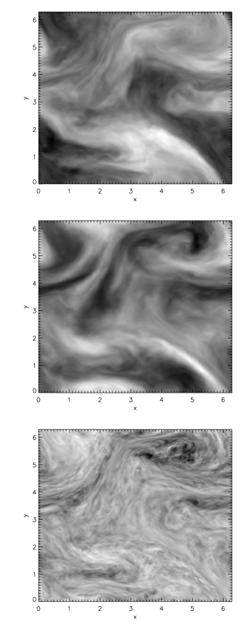
Figure 15: Horizontal average of the passive scalar (top), vertical velocity (middle) and vertical vorticity (bottom) for one snapshot of the fields at late times in run A2.

In figure 13 we show the PDFs of velocity and passive scalar derivatives (respectively $\partial_{x}u_{x}$ and $\partial_{x}\theta$), in run A1 ($\Omega=0$). Deviations from Gaussian statistics are observed for both derivatives. The PDFs of the derivatives $\partial_{x}\theta$ and $\partial_{x}u_{x}$ for run A2 ($\Omega\neq 0$) shown in Fig. 14 also present strong deviations from Gaussianity and asymmetry for $\partial_{x}\theta$. Calculation of the skewness for the PDFs of $\partial_{x}\theta$ shows a value of $S_{\theta}=0.04$ for run A1, and $S_{\theta}=-0.15$ for run A2. For velocity gradients, skewness is $S_{u}=-0.65$ for run A1, and $S_{u}=-0.44$ for run A2.

Since differences in the tails of the PDFs in the rotating and non-rotating cases may not be easily appreciated in the figures, Table 3 lists the skewness and kurtosis for several quantities computed for runs A1 and A2. For the scalar field, the skewness is close to zero for all quantities when $\Omega=0$, but it becomes negative and with larger absolute values in the presence of rotation. The kurtosis of all quantities studied decreases in the rotating case. For the velocity field, the skewness is negative in all cases, but substantially decreases in the presence of rotation. As for the passive scalar, kurtosis of quantities associated with the velocity field also decreases with rotation.

Many of the results shown indicate both the passive scalar and the velocity field become anisotropic in the runs with rotations. To illustrate this, Fig. 15 shows an horizontal average of the passive scalar, of the $z$-component of the velocity field, and of the $z$-component of the vorticity, at late times in run A2. Some correlations between the distribution of the three quantities can be identified, as the large scale configuration is very similar in the three cases. However, vertical vorticity develops structures at much smaller scales, as expected. A detailed analysis of spatial correlations between the fields, and of spatial (turbulent) diffusion of the passive scalar, is left for future work.

IV Conclusions

In this paper we analyzed data from direct numerical simulations of advection and diffusion of a passive scalar in a rotating turbulent flow. The results were compared with passive scalar dynamics in isotropic and homogeneous turbulence. To this end, simulations with spatial resolution of $512^{3}$ grid points were performed in a regular periodic grid using a pseudospectral method. Turbulence was sustained by an external random mechanical forcing. The forcing scale was changed to consider the case where energy was injected at the largest available scale in the computational domain, as well as the case where a small separation of scales between the forcing and the size of the box allowed for some inverse transfer of energy to develop in the rotating case. The main focus of our study was in the resulting scaling laws in spectral space, and in intermittency as measured from structure functions and scaling exponents.

The most important result of this work is that, in rotating flows at moderate Rossby number, all scaling exponents of the passive scalar except for one can be determined with good accuracy from Kraichnan’s model Kraichnan (1968, 1994) for a flow with dimensionality $d=2$ (at least up to the highest order considered here, and within the error bars of our study). The value of $d$ can be understood from the effect of rotation, which transfers the energy preferentially towards modes perpendicular to the rotation axis Cambon and Jacquin (1989); Waleffe (1992); Cambon et al. (1997) and makes the flow quasi-two-dimensional. Moreover, all exponents in Kraichnan’s model depend on the second order scaling exponent for the passive scalar $\zeta_{2}$. The value of this exponent can be determined from simple dimensional arguments, and we showed the value of $\zeta_{2}=0.5$ to be consistent with phenomenology and with the numerical results.

The other results include an analysis of scaling of the power spectrum of the passive scalar, which in the rotating case scales as $\sim k_{\perp}^{-3/2}$. This result seems to be independent of whether there is scale separation between the forcing scale and the largest scale in the box, or not. In the former case, it was also observed that while the energy develops an inverse transfer in the presence of rotation, the passive scalar does not. Measures of anisotropy based on the spectrum and on structure functions also indicate that the passive scalar is more anisotropic at small scales (scales smaller than the forcing scale) than the velocity, although at larger scales the passive scalar is more isotropic than the velocity field.

Finally, probability density functions of derivatives and longitudinal increments of the velocity field and of the passive scalar show a decrease of intermittency in the rotating case (as indicated, e.g., by a decrease in their kurtosis), more pronounced for the velocity than for the passive scalar. This is also in agreement with results obtained from the structure functions of the scalar and velocity field, as well as from the intermittency exponents for each field.