The Deformable Universe

Abstract

The concept of smooth deformations of a Riemannian manifolds, recently evidenced by the solution of the Poincar é conjecture, is applied to Einstein’s gravitational theory and in particular to the standard FLRW cosmology. We present a brief review of the deformation of Riemannian geometry, showing how such deformations can be derived from the Einstein-Hilbert dynamical principle. We show that such deformations of space-times of general relativity produce observable effects that can be measured by four-dimensional observers. In the case of the FLRW cosmology, one such observable effect is shown to be consistent with the accelerated expansion of the universe.

keywords:Geometry,Cosmology,Dark Energy,Geometric Flows

1 Introduction

The $\Lambda$CDM paradigm for the accelerated expansion of the universe makes use the cosmological constant $\Lambda$, interpreted as the vacuum energy density of quantum fields, as the main cause of the acceleration. However, it has been proven to be very difficult to explain the large difference between the very small observed value $\Lambda/8\pi G\approx 10^{-47}Gev^{2}/c^{4}$ and the very large averaged value of the quantum vacuum energy density $<\rho_{v}>\approx 10^{75}Gev^{2}/c^{4}$. The lack of a feasible explanation for such cosmological constant problem makes the $\Lambda$CDM paradigm unacceptable as a preferred theoretical option. In face of this difficulty a variety of alternative explanations have been proposed, including the possible existence of new and previously unheard of essences; the postulation of specific scalar fields; or even the possible existence of non observable extra dimensions in space.

The extra dimensional proposition is interesting because it may solve another fundamental issue, namely the hierarchy of the fundamental interactions, the huge ratio of the Planck to the electroweak energy scale ($M_{Pl}/M_{EW}\sim 10^{16}$). Indeed, Newton’s gravitational constant $G$ depends on the dimension of space. It has been shown that in a higher dimensional space the constant $G$ must change to another value $G_{*}$, such that gravitating masses can be correctly evaluated by a (higher dimensional) volume integration of given mass densities [1].

Yet, the hypothetical existence of extra dimensions must be compatible with the experimentally proven and mathematically consistent four-dimensionality of space-times. For example it took about 60 years to find out that the Kaluza-Klein theory based on the Einstein-Hilbert principle and having a product topology space, is not compatible with the observed fermion chirality at the electroweak scale, mainly because the diameter of the compact internal space is too small (the Planck length).

In a more recent proposal the product topology of the higher dimensional space has been replaced by an embedding space, while the Einstein-Hilbert principle was maintained and some other assumptions are introduced. The four-dimensionality of space-time is maintained, but the gravitational field propagates not only in the four-dimensional space-time but also along the extra dimensions. However the dynamics of this extra-dimensional propagation or deformation, has not been detailed and this is the main subject of this paper.

Several interesting models have been proposed, mostly belonging to the brane-world paradigm proposed in [1, 2], sometimes using additional conditions [3, 4], or other specific embedding assumptions as for example in e.g. [5, 6, 7, 8, 9, 10, 11, 12, 13, 14, 15]. In spite of such efforts we still do not have a model independent solution of the present cosmological problems [16].

The purpose of this paper is to study the dynamics of deformation of gravitational fields in arbitrary directions. We will see that such deformations are associated with a conserved quantity, the deformation tensor, which leads to an observable effect in space-time. We will show that the current observations on the acceleration of the universe are consistent with the observational effect of the deformation tensor.

2 Smooth Deformations of Space-times

The concept of smooth deformation of Riemannian manifolds was defined by John Nash as a means to correct the inability of the Riemann tensor to distinguish the local shape of the manifold. This problem lies at the foundations of Riemannian geometry and it is worth reviewing it, starting from Riemann’s own words as we quote: …We may, however, abstract from external relations by considering deformations which leave the lengths of lines within the surfaces unaltered, i. e, by considering arbitrary bendings -without stretching- of such surfaces, and by regarding all surfaces obtained from one another in this way as equivalent. Thus, for example, arbitrary cylindrical or conical surfaces count as equivalent to a plane… B. Riemann [17].

In the application of Riemannian geometry to Einstein’s gravitational theory, the observables of the gravitational field are determined by the eigenvalues of the Riemann tensor (or its trace-free Weyl tensor for pure gravitation), with respect to the zero gravitational field of the flat plane Minkowski space-time of special relativity. However as pointed out by Riemann, the same tensor also vanishes for cones, ruled hyperboloids, or for helicoidal space-times. This leads to the conclusion that in general relativity the differences between these shapes are not relevant to gravitation (see e.g. [18]). We will show that they can actually be detected by an observer in a four-dimensional space-time.

A general solution for the shape problem in Riemannian geometry was suggested by L. Schlaefli in 1871, proposing that all Riemannian manifolds must be embedded in a larger space, in such a way that their Riemann tensors would be compared with the geometry of the embedding space. Specifically, the local shape of a Riemannian manifold is obtained by the difference between the Riemann tensors of the embedded and the embedding manifolds (in the original proposition the embedding space was assumed to be flat) [19]. Most importantly, Riemannian geometry is recovered with the application of the inverse embedding map.

however, such solution of the shape problem in Riemannian geometry depends on solving the Gauss-Codazzi-Ricci equations, which are non-linear differential equations involving the metric, the extrinsic curvature and the third fundamental form as independent variables. They provide the necessary and sufficient conditions for the existence of the embedding functions for a given Riemannian manifold [20]. Until very recently only particular solutions of those equations were obtained with the help of positive power series expansions of the embedding functions differentiable or by try and error.

Nash’s theorem of 1956 changed this picture when he proposed that the metric of a given Riemannian manifold could be smoothly deformed along an orthogonal directions with parameter $y$, given by

$$k_{\mu\nu}=-\frac{1}{2}\frac{\partial g_{\mu\nu}}{\partial y}$$ (1)

where $k_{\mu\nu}$ denotes the extrinsic curvature and $y$ represents a coordinate on a direction orthogonal to the embedded geometry [21]. Thus, Nash’s theorem introduced the concept of deformable Riemannian manifolds in arbitrary directions, at the same time that it solved the embedding problem.

The condition (1) is a generalization of the well known York relation used in the study of the initial value problem for 3-dimensional surfaces in general relativity [22], to the case where $y$ is not necessarily the time coordinate. It is also analogous, but far more general than the “ Ricci flow” condition proposed much latter by R. Hamilton using the Fourier heat flux law to obtain the expression [24]

$$R_{\mu\nu}=-\frac{1}{2}\frac{\partial g_{\mu\nu}}{\partial y}$$

where $y$ represents any coordinate of a 3-dimensional manifold. This result was subsequently applied with success by G. Perelman to solve the Poincar é conjecture [25]. Unfortunately this condition is not relativistic and it is not compatible with Einstein’s equations or with relativistic cosmology. Indeed, together with Einstein’s equations, the above equations gives a linear equation for the gravitational field with respect to an arbitrary space-time direction $y$, strongly constraining the propagation of gravitation to

$$\frac{\partial g_{\mu\nu}}{\partial y}=-16\pi G(T_{\mu\nu}-\frac{1}{2}Tg_{\mu\nu})$$

On the other hand, (1) does not have such limitation because in each embedded space-time $g_{\mu\nu}$ and $k_{\mu\nu}$ are independent variables satisfying the Gauss-Codazzi-Ricci equations, instead of (LABEL:eq:Ricciflow). In the following we present a derivation of (1) for the simple case of just one extra dimension. Higher dimensional cases were also implicit in Nash’s paper, and it was applied as a possible extension of the ADM quantization of the gravitational field [26].

Consider a Riemannian manifold $\bar{V_{n}}$ with metric $\bar{g}_{\mu\nu}$, and its local isometric embedding in a D-dimensional Riemannian manifold $V_{D}$, $D=n+1$, given by a differentiable and regular map $\bar{X}:\bar{V}_{n}\rightarrow V_{D}$ satisfying the embedding equations

$$\bar{X}^{A}{}_{,\mu}\bar{X}^{B}{}_{,\nu}{\cal G}_{AB}=g_{\mu\nu},\;\bar{X}^{A}{}_{,\mu}\bar{\eta}^{B}{\cal G}_{AB}=0,\;\bar{\eta}^{A}\bar{\eta}^{B}{\cal G}_{AB}=1,\;A,B=1..D$$ (2)

where we have denoted by ${\cal G}_{AB}$ the metric components of $V_{D}$ in arbitrary coordinates, and where $\bar{\eta}$ denotes the unit vector field orthogonal to $\bar{V}_{n}$. The extrinsic curvature of $\bar{V}_{n}$ is by definition the projection of the variation of $\eta$ on the tangent plane [20]:

$$\bar{k}{}_{\mu\nu}=-\bar{X}^{A}{}_{,\mu}\bar{\eta}^{B}{}_{,\nu}{\cal G}_{AB}=\bar{X}^{A}{}_{,\mu\nu}\bar{\eta}^{B}{\cal G}_{AB}$$ (3)

The integration of the system of equations (2) gives the required embedding map $\bar{X}$.

Next, construct the one-parameter group of diffeomorphisms defined by the map $h_{y}(p):V_{D}\rightarrow V_{D}$, describing a continuous curve $\alpha(y)=h_{y}(p)$, passing through the point $p\in\bar{V_{n}}$, with unit normal vector $\alpha^{\prime}(p)=\eta(p)$. This group is characterized by the composition $h_{y}\circ h_{\pm y^{\prime}}(p)\stackrel{{\scriptstyle def}}{{=}}h_{y\pm y^{\prime}}(p)$, $h_{0}(p)\stackrel{{\scriptstyle def}}{{=}}p$. Applying this diffeomorphisms to all points of a neighborhood of $p$, with a smooth variation of the parameter $y$ (regardless if the parameter $y$ is time-like or not, or if it is positive or negative), we obtain a congruence of curves (the orbits of the group), all orthogonal to $\bar{V}_{n}$, describing a smooth flow of points in $V_{D}$, which may (or not) define the deformed manifold $V_{n}$.

Given a geometric object $\bar{\omega}$ in $\bar{V}_{n}$, its Lie transport along that flow for a small distance $\delta y$ is given by $\Omega=\bar{\Omega}+\delta y\pounds_{\eta}{\bar{\Omega}}$, where $\pounds_{\eta}$ denotes the Lie derivative with respect to $\eta$ [27]. In particular, take the Lie transport of the Gaussian frame $\{\bar{X}^{A}_{\mu},\bar{\eta}^{A}_{a}\}$ of the original manifold $\bar{V}_{n}$ obtaining

$$Z^{A}{}_{,\mu} = X^{A}{}_{,\mu}+\delta y\;\pounds_{\eta}{X^{A}{}_{,\mu}}=X^{A}{}_{,\mu}+\delta y\;\eta^{A}{}_{,\mu}$$ (4)

$$\eta^{A} = \bar{\eta}^{A}+\delta y\;[\bar{\eta},\bar{\eta}]^{A}\;\;\;\;\;\;=\;\;\bar{\eta}^{A}$$ (5)

However, it should be noted from (3) that in general $\eta_{,\mu}\neq\bar{\eta}_{,\mu}$.

The set of coordinates $Z^{A}$ obtained by integrating these equations does not necessarily describe another manifold. In order to be so, they need to satisfy embedding equations similar to (2):

$$Z^{A}{}_{,\mu}Z^{B}{}_{,\nu}{\cal G}_{AB}=g_{\mu\nu},\;Z^{A}{}_{,\mu}\eta^{B}{\cal G}_{AB}=0,\;\eta^{A}\eta^{B}{\cal G}_{AB}=1$$ (6)

Replacing (4) and (5) in (6) and using the definition (3) we obtain the metric and extrinsic curvature of the new manifold

$$g_{\mu\nu}=\bar{g}_{\mu\nu}-2y\bar{k}_{\mu\nu}+y^{2}\bar{g}^{\rho\sigma}\bar{k}_{\mu\rho}\bar{k}_{\nu\sigma}$$ (7)

$$k_{\mu\nu}=\bar{k}_{\mu\nu}-2y\bar{g}^{\rho\sigma}\bar{k}_{\mu\rho}\bar{k}_{\nu\sigma}$$ (8)

It is easy to see that Nash’s deformation condition (1) follows from the derivative of (7) with respect to $y$ and comparing the result with (8).

Of course, in order to define a new differentiable manifold, equations (6) need to be integrated. The integrability conditions for these equations are intimately associated with the differentiable (smooth) properties of the embedding functions, providing the proposed solution of the shape problem. That is, the components of the Riemann tensor of the embedding space, are evaluated in the Gaussian frame $\{Z^{A}_{\mu},\eta^{A}\}$

$${}^{5}{\cal R}_{ABCD}Z^{A}{}_{,\alpha}Z^{B}{}_{,\beta}Z^{C}{}_{,\gamma}Z^{D}{}_{,\delta}=R_{\alpha\beta\gamma\delta}+\!\!(k_{\alpha\gamma}k_{\beta\delta}\!-\!k_{\alpha\delta}k_{\beta\gamma})\!\!$$ (9)

$${}^{5}{\cal R}_{ABCD}Z^{A}{}_{,\alpha}Z^{B}{}_{,\beta}Z^{C}{}_{,\gamma}\,\eta^{D}=k_{\alpha[\beta;\gamma]}$$ (10)

We obtain the Gauss-Codazzi equations [20]. The first of these equation (the Gauss equation) clearly shows that the Riemann curvature of the embedding space acts as a reference for the Riemann curvature of the embedded space-time. It is true that both Riemann curvature tensors carry the same shape problem in the sense described by Riemann, but the differences between the two Riemann tensors given by the extrinsic curvature defines the shape of the embedded geometry. The second equation (Codazzi) complements this interpretation, stating that projection of the Riemann tensor of the embedding space along the normal direction is given by the tangent variation of the extrinsic curvature. Although the normal vector $\eta$ is not observable, the extrinsic curvature is quantity defined in space-time. A third equation, the Ricci equation , is a trivial identity in the case of just one extra dimension (hypersurfaces).

3 Deformation Dynamics

Equations (7) and (8) describe the metric and extrinsic curvature of the deformed geometry ${V}_{4}$. By varying $y$ they can describe a continuous sequence of deformed geometries. The existence of these deformations are given by the integrability conditions (9) and (10). as such these equations must not be confused with dynamical equations.

As in Kaluza-Klein and brane-world theories, the embedding space $V_{5}$ has a metric geometry defined by the higher-dimensional Einstein’s equations

$${}^{5}{\cal R}_{AB}-\frac{1}{2}\,{{}^{5}{\cal R}}{\cal G}_{AB}=G_{*}T^{*}_{AB}$$ (11)

where $G_{*}$ is the new gravitational constant and where $T^{*}_{AB}$ are components of the energy-momentum tensor of the known material sources. These equations are derived from the Einstein-Hilbert principle, to which we give a natural interpretation: the space-times satisfying (11) are those with the smoothest Riemannian curvature.

$$\delta\int{{}^{5}{\cal R}}\sqrt{\cal G}dv=0$$

From (11) we may derive the gravitational field in the embedded space-times, after the following observations
1) A cosmological constant was not included in (11), so that the existence of an embedded 4-dimensional Minkowski space-time (A cosmological constant was included in [23], but here we see no reason for it.). With this choice we also ensure that the cosmological constant problem does not appear.
2) The confinement of the gauge fields to four dimensions is not an assumption, but a consequence of the fact that only in four dimensions the three-form resulting from the derivative of the Yang-Mills curvature tensor is isomorphic to the one-form current. Consequently, all known observable sources of gravitation composing $T_{AB}$ are necessarily confined to four-dimensional embedded space-times. Such confinement can be implemented a very simple way by writing Einstein’s equation (11) in the Gaussian frame of every space-time with the energy-momentum tensor source $T_{\mu\nu}$ is such that

$$8\pi GT_{\mu\nu}=G_{*}Z^{A}_{,\mu}Z^{B}_{,\nu}T^{*}_{AB},\;\;\;Z^{A}_{,\mu}\eta^{B}T^{*}_{AB}=0,\;\;\;\mbox{and}\;\;\eta^{A}\eta^{B}T^{*}_{AB}=0$$ (12)

3) The set of all deformations of a given space-time generates a continuous foliation of the embedding space, composed by four-dimensional space-times, parameterized by the extra dimension $y$. For each fixed value of $y$, we obtain a deformed space-time which, if so desired can be de-embedded, with the application of the local inverse embedding map, which always exists provided the embedding is regular. In this way we may recover the purely intrinsic Riemannian geometry. In some models the addition of extra conditions may prevent not only the construction of the foliation, but also the recovery of the Riemannian structure. One particular class of models (e.g. [3, 4]) uses the Israel-Lanczos boundary condition [28]

$$k_{\mu\nu}=G_{*}(T_{\mu\nu}-\frac{1}{3}Tg_{\mu\nu})$$ (13)

When applying Nash’s deformation we cannot have such condition. In the first place because it fixes once for all the value of the extrinsic curvature in terms of the confined sources, thus preventing the application of (1). The condition (13) is also limited to hypersurfaces, so that if the embedding requires additional dimensions it does not apply. In addition to obtain (13) we also require a special that the embedded space-time is a fixed boundary between two sides of the embedding space with mirror symmetry. To see this, consider Einstein’s equations in five dimensions, (11) which can be written as

$${}^{5}{\cal R}_{AB}=G_{*}(T^{*}_{AB}-\frac{1}{3}T^{*}{\cal G}_{AB})$$ (14)

the left hand side may be evaluated in the embedded space-time frames by contracting it with $Z^{A}_{,\mu}Z^{B}_{,\nu}$, using (1), (6) and the confinement conditions (12), obtaining the tangent components

$${}^{5}{\cal R}_{\mu\nu}=R_{\mu\nu}+\frac{\partial k_{\mu\nu}}{\partial y}-2k_{\mu\rho}k^{\rho}_{\nu}+hh_{\mu\nu}=8\pi G_{*}(T_{\mu\nu}-\frac{1}{2}Tg_{\mu\nu})\\$$ (15)

As we can see, (15) does not coincide with (13). In order to obtain the Israel-Lanczos condition from the above equations it becomes necessary to fix the embedding, say at $y=0$; find the values of (15) on both sides and finally evaluate the difference between these values. We find that all tangent components cancel, except the terms $\partial k_{\mu\nu}/\partial y$, which add when the $y$ change sign from one side to another of the boundary $y=0$. Finally, by integrating that difference in $y$, using a Dirac’s function on $y=0$, we obtain (13). In some models motivated by string theory, the condition (13) is imposed upfront, making it impossible to conciliate those models with Nash’s deformations.

With these remarks we may proceed with the deformation dynamics, now contracting (11) in its original form with $\{Z^{A}_{,\mu},\eta^{A}\}$ using (6) and the confinement conditions obtaining two gravitational equations (These are the same equations derived in [23])

$$R_{\mu\nu}-\frac{1}{2}Rg_{\mu\nu}-Q_{\mu\nu}=8\pi GT_{\mu\nu}\;\hskip 5.69054pt$$ (16)

$$k_{\mu;\rho}^{\;\rho}-h_{,\mu}=0\;,\hskip 139.41832pt$$ (17)

where $h^{2}=g^{\mu\nu}k_{\mu\nu}$ is the (squared) mean curvature and $K^{2}=k^{\mu\nu}k_{\mu\nu}$ is the (squared) Gauss curvature and where the term $Q_{\mu\nu}$ is

$$Q_{\mu\nu}=g^{\rho\sigma}k_{\mu\rho}k_{\nu\sigma}-k_{\mu\nu}h-\frac{1}{2}\left(K^{2}-h^{2}\right)g_{\mu\nu}\;,$$ (18)

This geometrical quantity called the deformation tensor is conserved in the sense of

$$Q^{\mu\nu}{}_{;\nu}=0\;.$$ (19)

This means that there are observables effects associated with the extrinsic curvature in the four-dimensional space-time.

To understand the nature of the observables associated with the extrinsic curvature, consider again the one-parameter group of diffeomorphism defined by points in an embedded space-time, and the unit normal vector $\eta$, with orbit $\alpha(y)=h_{y}(p)$. The Frenet equation for this orbit tells that there is a transverse acceleration orthogonal to its velocity $\eta$, which is therefore tangent to the embedded space-time. As such, this vector can be written as a a linear combination of the tangent basis $\{Z^{A}_{,\mu}\}$ expressed as

$$\eta^{A}_{,\mu}=g^{\rho\sigma}k_{\mu\rho}Z^{A}_{,\sigma}$$ (20)

As it happens, except for a difference in sign this is the definition of the extrinsic curvature (see e.g. [20].). Therefore, the presence of the extrinsic curvature associated with (1) represents an acceleration tangent to space-time. Since such acceleration always points to the concave side of the curve, then in the case of a deformation with volume expansion, it implies in the emergence of the Riemann stretching on the space-time geometry, which in principle can responsible for the accelerated expansion of the universe.

Nash’s deformation condition (1) tells how the embedding space can be filled by a continuous succession of deformed space-times, each one given by a fixed value of $y$. In each of these space-times the metric $g_{\mu\nu}$ and the extrinsic curvature $k_{\mu\nu}$ are independent variables satisfying the Gauss-Codazzi equations. Therefore each of them requires the determination of 20 unknowns, whereas counting from (11) we have only 15 dynamical equations. If we ignore $k_{\mu\nu}$ in (16), we obtain the usual Einstein’s equations for the metric $g_{\mu\nu}$, suggesting that the missing equations describe the extrinsic curvature.

Since $k_{\mu\nu}$ is a symmetric rank-2 tensor, it corresponds also to a spin-2 field whose dynamics is determined by a well known theorem due to S. Gupta. It tells that any such tensor necessarily satisfy an Einstein-like system of equations, having the Pauli-Fierz equation as its linear approximation [29, 30, 31]. The original theorem of Gupta was set in the Minkowski space-time. Here we need to derive Gupta’s equations for the extrinsic curvature in a deformed space-time with metric $g_{\mu\nu}$.

Using an analogy with the derivation of Einstein’s equations, we start by noting that $k_{\mu\nu}k^{\mu\nu}=K^{2}\neq 4$, so that we need to normalize the extrinsic curvature, defining a temporary tensor

$$f_{\mu\nu}=\frac{2}{K}k_{\mu\nu},$$ (21)

and define its inverse by $f^{\mu\rho}f_{\rho\nu}=\delta^{\mu}_{\nu}$. It follows that $f^{\mu\nu}=\frac{2}{K}k^{\mu\nu}$.

Denoting by $||$ the covariant derivative with respect to a connection defined by $f_{\mu\nu}$, while keeping the usual semicolon notation for the covariant derivative with respect to $g_{\mu\nu}$, the analogous to the “Levi-Civita” connection associated with $f_{\mu\nu}$ such that ” $f_{\mu\nu||\rho}=0$, is:

$$\Upsilon_{\mu\nu\sigma}=\;\frac{1}{2}\left(\partial_{\mu}\;f_{\sigma\nu}+\partial_{\nu}\;f_{\sigma\mu}-\partial_{\sigma}\;f_{\mu\nu}\right)$$ (22)

Defining

$$\Upsilon_{\mu\nu}{}^{\lambda}=f^{\lambda\sigma}\;\Upsilon_{\mu\nu\sigma}$$

The “Riemann tensor” for $f_{\mu\nu}$ has components

$${\cal F}_{\nu\alpha\lambda\mu}=\;\partial_{\alpha}\Upsilon_{\mu\lambda\nu}-\;\partial_{\lambda}\Upsilon_{\mu\alpha\nu}+\Upsilon_{\alpha\sigma\mu}\Upsilon_{\lambda\nu}^{\sigma}-\Upsilon_{\lambda\sigma\mu}\Upsilon_{\alpha\nu}^{\sigma}$$

and the analogous to the “Ricci tensor” and the “Ricci scalar” for $f_{\mu\nu}$ are, respectively given by

$${\cal F}_{\mu\nu}=f^{\alpha\lambda}{\cal F}_{\nu\alpha\lambda\mu}\;\;\mbox{and}\;\;{\cal F}=f^{\mu\nu}{\cal F}_{\mu\nu}$$

Finally, Gupta’s equations for $f_{\mu\nu}$ can be obtained from the contracted Bianchi identity

$${\cal F}_{\mu\nu}-\frac{1}{2}{\cal F}f_{\mu\nu}=\;\alpha_{*}\mathcal{T}_{\mu\nu}$$ (23)

where $\mathcal{T}_{\mu\nu}$ represents the source of this field such that $\mathcal{T}^{\mu\nu}{}_{||\nu}=0$ and $\alpha_{*}$ is a coupling constant. Notice that in spite of the resemblances, $k_{\mu\nu}$ is not a metric because it exists only after the Riemannian geometry with the metric $g_{\mu\nu}$ has been defined for the metric $g_{\mu\nu}$.

4 Deforming the FLRW Universe

As we have seen Nash’s deformations of a space-time defined by the extrinsic curvature satisfying Gupta’s equation produces a tangent acceleration in space-time. We have seen also that the same extrinsic curvature produces an observable quantity $Q_{\mu\nu}$. Such reasoning non-trivial sequence suggests that the currently observed acceleration of the distant supernovae type Ia (SN Ia), can be related to the deformations of the standard FLRW universe, something that has to be experimentally verified.

For that purpose consider the line element of the FLRW universe written as

$$ds^{2}=g_{\alpha\beta}dx^{\alpha}dx^{\beta}=-dt^{2}+a^{2}[dr^{2}+f(r)(d\theta^{2}+sen^{2}\theta d\varphi^{2})]$$

where $f(r)=\sin r,r,\sinh r$ corresponds to the spatial curvature $k=1,0,-1$ respectively. The the confined source is the perfect fluid given in co-moving coordinates written as

$$T_{\alpha\beta}=(p+\rho)U_{\alpha}U_{\beta}+pg_{\alpha\beta},\;\;U_{\alpha}=\delta_{\alpha}^{4}.$$ (24)

The embedding of the FLRW universe in a five dimensional flat space gives the solution (details in [23])

$$k_{ij}=\frac{b}{a^{2}}g_{ij},\;\;i,j=1,2,3,\;\;\;\;k_{44}=\frac{-1}{\dot{a}}\frac{d}{dt}\frac{b}{a}\;,$$ (25)

Just for notational simplicity denote $b=-k_{11}$, $\xi=k_{44}$, $H=\dot{a}/a$ and $B=\dot{b}/b$. Then the components of the extrinsic geometry can be written as

$$\xi=\frac{b}{a^{2}}(\frac{B}{H}-1)g_{44},\;\;$$ (26)

$$K^{2}=\frac{b^{2}}{a^{4}}\left(\frac{B^{2}}{H^{2}}-2\frac{B}{H}+4\right),\;\;\,h=\frac{b}{a^{2}}(\frac{B}{H}+2)$$ (27)

$$Q_{ij}=\frac{b^{2}}{a^{4}}\left(2\frac{B}{H}-1\right)g_{ij},\;\quad\quad Q_{44}=-\frac{3b^{2}}{a^{4}},$$ (28)

$$Q=-(K^{2}-h^{2})=\frac{6b^{2}}{a^{4}}\frac{B}{H}\;,$$ (29)

Replacing the above results in (16) we obtain the Friedman equation modified by the presence of the extrinsic curvature, i.e.,

$$\left(\frac{\dot{a}}{a}\right)^{2}+\frac{\kappa}{a^{2}}=\frac{8}{3}\pi G\rho+\frac{b^{2}}{a^{4}}$$ (30)

To complete the set of dynamical equations we use (23). Applying (25) to the definition (21) we obtain for the FLRW metric

$$f_{ij}=\frac{2}{K}g_{ij},\;i,j=1..3,\;\;\;f_{44}=-\frac{2}{K}\frac{1}{\dot{a}}\frac{d}{dt}{\left(\frac{b}{a}\right)}$$ (31)

where the function $b(t)=k_{11}$ remains undefined. To find it we submit it to (23). The main difficulty here is the determination of the source ${\cal T}_{\mu\nu}$ of that equation for, if for no other philosophical reasons (e.g. if the universe expands, it expands to where?), we have no previous experience on the dynamics of space-time deformations. In this case, the correct procedure is to look for models that fit the experimental data on the expansion of the universe, as for example the perfect fluid used in [23]. However, within the context of a geometry and topology of the universe determined by the observations, the acceleration of the universe can be seen as a the observable effect associated with the deformation of the universe defined by the extrinsic curvature. The simplest option for the external source of equation (23) is the void characterized by $\mathcal{T}_{\mu\nu}=0$. We regard this a a first attempt to see where such reasoning leads us.

The Ricci-flat-like equation (23) becomes simply

$${\cal F}_{\mu\nu}=0$$ (32)

From (31) we derive the components of (22); of the f-curvature ${\cal F}_{\mu\nu\rho\sigma}$ and finally write the Ricci-flat equation (32), whose components ${\cal F}_{\mu\nu}$ in this particular example are

$$\mathcal{F}_{11}=\frac{1}{4}\frac{-4b^{2}\xi\dot{K}^{2}\!+\!5b\xi\dot{K}\dot{b}K-\dot{b}^{2}\xi K^{2}+2b^{2}\xi K\ddot{K}-2b\ddot{b}\xi K^{2}-b^{2}\dot{K}\dot{\xi}K+bK^{2}\dot{b}\dot{\xi}}{\xi^{2}K^{2}b}=0$$ (33)

$$\mathcal{F}_{22}=r^{2}\frac{-4b^{2}\xi\dot{K}^{2}+5b\xi\dot{K}\dot{b}K-\dot{b}^{2}\xi K^{2}+2b^{2}\xi K\ddot{K}-2b\ddot{b}\xi K^{2}-b^{2}\dot{K}\dot{\xi}K+bK^{2}\dot{b}\dot{\xi}}{4\xi^{2}K^{2}b}=0$$ (34)

$$\mathcal{F}_{33}=\sin^{2}(\theta)\mathcal{F}_{22}=0$$ (35)

$$\mathcal{F}_{44}=-\frac{3}{4}\frac{\dot{b}^{2}\xi K^{2}+2b^{2}\xi K\ddot{K}-2b\ddot{b}\xi K^{2}-b^{2}\dot{K}\dot{\xi}K+bK^{2}\dot{b}\dot{\xi}-2b^{2}\xi\dot{K}^{2}+b\xi K\dot{K}\dot{b}}{\xi K^{2}b^{2}}=0$$ (36)

The only essential equations in the above set are the first and last equations. By subtracting these equations we obtain $b^{2}\dot{K}^{2}+K^{2}\dot{b}^{2}=2bK\dot{b}\dot{K}$ or, equivalently,

$$\left(\frac{\dot{K}}{K}\right)^{2}-2\frac{\dot{b}}{b}\frac{\dot{K}}{K}=-\left(\frac{\dot{b}}{b}\right)^{2}$$ (37)

which has a simple solution $K(t)=2\eta_{0}b(t)$, where we have denoted by $2\eta_{0}$ its integration constant. Replacing the expression of $K$ given by (27), we obtain

$$\frac{B}{H}=1\pm\sqrt{4\eta_{0}^{2}a^{4}-3}$$ (38)

Of course, to obtain real values of $a$ and $b$, we must have the condition

$$\eta_{0}^{2}\geq\frac{3}{4}\frac{1}{a^{4}}$$ (39)

Expressing $Q_{\mu\nu}$ in terms of $B/H$ given by (28), the conservation equation (19) can be readily integrated giving

$$2\frac{B}{H}-1=\beta_{0}$$ (40)

where $\beta_{0}$ is a second integration constant.

Subtracting (40) from (38), we obtain the searched equation on $b(t)$ expressed as a function of the expansion parameter $a(t)$

$$\frac{\dot{b}}{b}=\frac{\dot{a}}{a}(\beta_{0}\mp\sqrt{4\eta_{0}^{2}a^{4}-3})$$ (41)

The integration of which is very simple. Merging all integration constants into a single one $\alpha_{0}$ the final solution can be expressed as

$$b(t)=\alpha_{0}a^{\beta_{0}}e^{\mp\gamma(a)}$$ (42)

where $\gamma(a)$ is given by

$$\!\!\gamma(a)=\!\!\sqrt{4\eta_{0}^{2}a^{4}-3}-\!\sqrt{3}\arctan\left(\frac{\sqrt{3}}{3}\sqrt{4\eta_{0}^{2}a^{4}-3}\right)$$ (43)

Replacing (39) and (42) in (30) we obtain the Friedman equation modified by the extrinsic curvature:

$$\left(\frac{\dot{a}}{a}\right)^{2}+\frac{\kappa}{a^{2}}=\frac{4}{3}\pi G\rho+\frac{\alpha_{0}^{2}a^{2\beta_{0}}e^{\mp 2\gamma(a)}}{a^{4}}$$ (44)

As we see the result depends on a choice of three integration constants $\alpha_{0}$, $\beta_{0}$ and $\eta_{0}$ which must be adjusted by known boundary conditions:

(a) The constant $\alpha_{0}$ is a scale factor for $b(t)$ which can be fixed once for all for today’s ($t=0$) value to be $\alpha_{0}=1$, by setting $b(0)=a^{\beta}_{0}(0)e^{\mp\gamma(a=1)}$, where we have denoted today’s value of

$$e^{\gamma\,(a=1)}=\sqrt{4\eta_{0}^{2}-3}-\sqrt{3}\arctan\left(\frac{\sqrt{3}}{3}\sqrt{4\eta_{0}^{2}-3}\right)$$

(b) The equal sign in (39) gives $\gamma(a)=0$, which corresponds to the particular case previously studied in our previous paper [23], where a comparison of the extrinsic curvature with a phenomenological fluid (the X-fluid) was used. In the following we consider the more general cases corresponding to the greater sign ($>$) in (39).

In order to evaluate the above results with the presently available data we translate the equations in terms of the redshift $z$, when the expansion parameter becomes $a(z)=1/(1+z)$ and the condition (39) becomes $\eta_{0}^{2}\geq\frac{3}{4}(1+z)^{4}$. Furthermore, we express (44) in terms of the relative densities $\Omega_{k},\;\Omega_{\Lambda},\;\Omega_{matter}=\Omega_{m},\;\Omega_{extrinsic}=\Omega_{ext}$, with the following observations.

(1) Since the value of the spatial curvature $\kappa$ in (44) has been consistently verified to be zero [32], we will simple ignore the contribution of $\Omega_{k}$.

(2) From our previous arguments on the cosmological constant problem we have eliminated the cosmological constant contribution in this analysis, so that we also take $\Omega_{\Lambda}=0$. We will see that the contribution of $\Lambda$ is not really relevant to the accelerated expansion in presence of the contribution of the extrinsic curvature.

(3) The baryonic matter relative density is denoted by $\Omega_{m}$ and the extrinsic relative density is denoted by $\Omega_{\rm ext}$. Assuming the standard normalization condition $H\rfloor_{z=0}=H_{0}=100h\;km.s^{-1}\;Mpc^{-1}$ (the Hubble constant), we may write these in terms of $z$ as

$$\Omega_{m}=\frac{8\pi G}{3\rho(1+z)^{3}}\;\;\mbox{and}\;\;\Omega_{\rm{ext}}=\frac{1-\Omega_{m}}{e^{\gamma\,(z=0)}}$$ (45)

With these considerations the modified Friedman equation (44) written in terms of the redshift becomes

$${{E(z)}}=\frac{\dot{a}(z)}{a(z)}=\left[\Omega_{m}(1+z)^{3}+{\Omega_{\rm{ext}}(1+z)^{4-2\beta_{0}}}\right]^{1/2}$$ (46)

To find if this result corresponds to the observations we use a statistical analysis which gives a model independent probe of the accelerating expansion of the universe [32]. This is given by the dimensionless luminosity-distance expression

$$d_{L}(z)=(1+z)\frac{\int_{0}^{z}\frac{dz^{\prime}}{E(z^{\prime})}}{H_{0}}$$ (47)

For the two considered density parameters $\Omega_{m}$ and $\Omega_{\rm{ext}}$, the luminosity distance is related to the distance modulus (with $d_{L}(z)$ measured in Mpc) as

$$\mu(z,u)=m-M=5\,log\,d_{L(z)}+25$$

where the parameters $m$ and $M$ represent respectively the apparent and absolute bolometric magnitudes [33].

We may evaluate the contribution of the extrinsic curvature by plotting the contours in the planes $(\Omega_{m},\beta_{0})$ for different values of $\eta_{0}$.

For the SN Ia database, the best fit values is given by the likelihood analysis is based on the calculation of the standard distribution

$$\chi^{2}(u)=\sum^{115}_{i=1}\frac{\left[\mu^{i}_{p}(z|\mathbf{u})-\mu^{i}_{0}(z|\mathbf{u})\right]^{2}}{\sigma^{2}_{i}}$$

where $\mu^{i}_{0}(z|\mathbf{u})$ is the extinction corrected distance modulus for a given SNe Ia at $z_{i}$ and $\sigma_{i}$ is the standard deviation of the uncertainty in the individual distance moduli (including uncertatinties in galaxy red shifts). The above summation was taken over the 115 observational Hubble data for SN Ia at redshifts $z_{i}$ [34] (For more details on such SN Ia statistical analysis we refer the reader to [35, 36, 37, 38, 39, 40, 41] and refs. therein.). We may estimate the admissible values of $\beta_{0}$ for the best fit values of the known data set on SN Ia in the parametric plane $(\Omega_{m},\beta_{0})$, with constant $\Delta\chi^{2}=2.30,\;\;6.17,\;\;11.8$, respectively for $\eta_{0}=3.5,5.0,7.0$, corresponding to the above mentioned 115 observations. The first value $\eta_{0}>3.5$ was taken from (39). The other two values, i.e., $\eta_{0}=5.0$ and $\eta_{0}=7.0$ were taken arbitrarily in the sequence.

Using data from [34] and since the highest-$z$ supernova Ia in our sample is at $z\simeq 1.01$ at 68.3% (C.L.) we have found for the three above values of for $\eta_{0}$, respectively

$$\mbox{for}\;\;\eta_{0}=3.5,\quad\beta_{0}=-1.45^{+0.30}_{-0.25}\quad\mbox{and}\quad\Omega_{m}=0.14\pm 0.03\;,$$

$$\mbox{for}\;\;\eta_{0}=5.0,\quad\beta_{0}=-3.09^{+0.5}_{-0.4}\quad\mbox{and}\quad\Omega_{m}=0.20\pm 0.03\;,$$

$$\mbox{for}\;\;\eta_{0}=7.0,\quad\beta_{0}=-5.35^{+0.7}_{-0.6}\quad\mbox{and}\quad\Omega_{m}=0.24\pm 0.03\;.$$

By combining the above results with the normalized expression in (45), we may estimate that the extrinsic curvature density parameter lies in the interval

$$10^{-2}\geq\Omega_{\rm{ext}}\geq 10^{-6}$$

showing that there is a wide range of the parameters for the extrinsic curvature density which fit the observations.

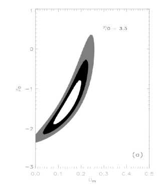
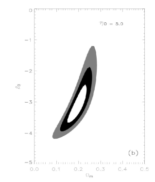
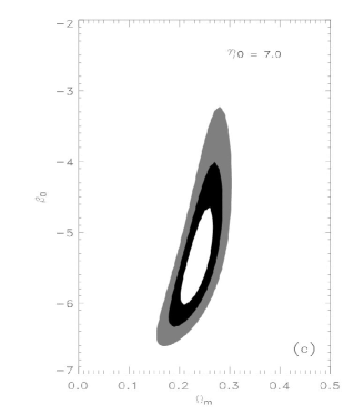
Figure 1: Contours of the $\chi^{2}$ test in the parametric space $\Omega_{m}$ (horizontal axis) versus $\beta_{0}$ (vertical axis). The contours are drawn for $\Delta\chi^{2}=2.30$, $6.17$ and $11.8$. As explained in the text, the value of $\eta_{0}$ has been fixed at 3.5 (a), 5.0 (b) and 7.0 (c). In particular, we note that for $\eta_{0}=7.0$, the allowed $\sigma$ interval for the matter density parameter is very close to that provided by current dynamical estimates, i.e., $\Omega_{m}\simeq 0.2-0.3$.

As a last remark we note that the contribution of the extrinsic curvature is also consistent with the expected age of the universe. This can be seen directly from (46), from which we extract the the age of the universe

$$t=\frac{-1}{H_{0}}\int{\frac{dz}{(1+z)\sqrt{\Omega_{m}(1+z)^{3}+\Omega_{\rm ext}(1+z)}}}$$

From this expression we conclude from the contour (b) in the above figure that for $0.14\leq\Omega_{m}\leq 0.3$, we obtain the age of the universe between $12\leq t\leq 16$, which is compatible with the estimated formation of the large structures [42].

Summary

We have applied the concept of smoothly deformable Riemannian manifolds to relativistic cosmology. The concept is similar to the one used by Perelman’s solution of the Poincar é conjecture, but where we applied Nash’s deformation instead of the Ricci flow. The advantage Nash’s geometric flow condition over the Ricci flow is that it is entirely relativistic and compatible with Einstein’s equations. However, Nash’s geometric description involve a new variable, the extrinsic curvature, so that it also requires a new dynamical process.

With basis in the spin-statistic theorem we have suggested an Einstein-like dynamical equation for the extrinsic curvature adapted from the original equation of S. Gupta. The result for a massless spin-2 field show that the when the deformation of the geometry produced by the extrinsic geometry is applied to the universe, we obtain a consistency with the current observations. We have applied a model independent statistical analysis, showing that the cosmological constant does not play a significant role on the acceleration of the universe in presence of the deformation, at least within the present observational range.

The deformation process defined by Nash requires the embedding of the space-time in a larger space. However, since the standard gauge fields which are required for our experimental basis are defined only in four-dimensions, the end result is a four-dimensional deformed space-time which is obtained by the inverse embedding map. The four-dimensional observers with its gauge field based technology will measure the end effects of the deformations without being aware of the embedding.

The presence of the extrinsic curvature leads also to a new conserved quantity the deformation tensor $Q_{\mu\nu}$, and so to an observational effect which adds some topological qualities to Einstein’s gravitation theory. This interpretation is supported by the Gauss and Riemann views that the true geometry will at the end be determined by the observations. Our estimates suggest that the observed acceleration of the universe evidences the existence of a deformation at the cosmological scale, giving to the universe some notion of its shape.

References

- [1] N. Arkani-Hamed et al., Phys. Lett. B429, 263 (1998).
- [2] V. A. Rubakov and M. Shaposhnikov, Phys. Lett. B 125, 136 (1983).
- [3] L. Randall and R. Sundrum, Phys. Rev. Lett. 83, 3370,(1999).
- [4] L. Randall and R. Sundrum, Phys. Rev. Lett. 83, 4690 (1999).
- [5] G. Dvali, G. Gabadadze and M. Porrati, Phys. Lett. B485, 208 (2000)
- [6] V. Sahni and Y. Shtanov, IJMP D11, 1515 (2002).
- [7] V. Sahni and Y. Shtanov, JCAP 0311, 014 (2003).
- [8] T. Shiromizu, K. Maeda, and M. Sasaki, Phys. Rev. D62, 024012 (2000).
- [9] R. Dick, Class. Quant. Grav. 18, R1 (2001).
- [10] C. J. Hogan, Class. Quant. Grav. 18, 4039 (2001).
- [11] C. Deffayet, G. Dvali and G. Gabadadze, Phys. Rev. D65, 044023 (2002).
- [12] J. S. Alcaniz, Phys. Rev. D 65, 123514 (2002).
- [13] D. Jain, A. Dev and J. S. Alcaniz, Phys. Rev. D66, 083511 (2002).
- [14] A. Lue, Phys. Rept. 423, 1 (2006).
- [15] M. Heydari-Fard, M. Shirazi, S. Jalalzadeh and H. R. Sepangi, Phys. Lett. B 640, 1 (2006).
- [16] H. F. Goenner, arxiv.org 0910.4333v2 (2010). .
- [17] B. Riemann, On the Hypothesis That Lie at the Foundations of Geometry (1854), translated by W. K. Clifford, Nature, 8,114 (1873). See also comments in P. Pesic, Beyond Geometry, Dover (2007).
- [18] C. W. Misner, Kip S. Thorne, & John A. Wheeler, Gravitation , W. H. Freeman Co. (1970)
- [19] L. Schlaefli, Annali di Matatematica ( series), 5, 170-193 (1871)
- [20] L. P. Eisenhart, Riemannian Geometry, Pinceton U. P. (1966)
- [21] J. Nash, Ann. Maths. 63, 20 (1956)
- [22] J. W. York Jr. Phys. Rev. Lett. 26, 1656, (1971).
- [23] M. D. Maia, E. M. Monte, J. M. F. Maia and J. S. Alcaniz, Class. Quant. Grav. 22, 1623 (2005). See also M. D. Maia, E. M. Monte and J. M. F. Maia, Phys. Lett. B585, 11 (2004).
- [24] R. Hamilton, J. Diff. Geom 17 (1982), 255 306.
- [25] G. Perelman arXiv:math/0211159
- [26] M. D. Maia, N. Silva and, M. C. B. Fernandes, JHEP 047, 0704 (2007).
- [27] M. Crampin and F.A. E. Pirani, Applicable Differential Geometry, Cambridge UP, (1986).
- [28] W. Israel, Nuovo Cimento 44, 4349 (1966)
- [29] C. J. Isham, A. Salam and J. Strathdee. Phys. Rev. 3, 4 (1971).
- [30] S. N. Gupta, Phys. Rev. 96, (6) (1954)
- [31] C. Fronsdal, Phys. Rev. D18 3624 (1978)
- [32] D. N. Spergel et al., Astrophys. J. Supl. 170, 377 (2007)
- [33] Lixin Xu et al, JCAP07 031 (2009), doi:10.1088/1475-7516/2009/07/031
- [34] P. Astier et al., Astron. Astrophys. 447, 31 (2006)
- [35] T. Padmanabhan and T. R. Choudhury, Mon. Not. R. Astron. Soc. 344, 823 (2003)
- [36] P. T. Silva and O. Bertolami, Astrophys. J. 599, 829 (2003)
- [37] Z. H. Zhu and J. S. Alcaniz, Astrophys. J. 620, 7 (2005)
- [38] J. S. Alcaniz, Phys. Rev. D 69, 083521 (2004).
- [39] T. R. Choudhury and T. Padmanabhan, Astron. Astrophys. 429, 807 (2005).
- [40] M. Kowalski et al., Astrophys. J. 686, 749 (2008)
- [41] L. Samushia and B. Ratra, Astrophys. J. 650, L5 (2006)
- [42] E. Komatsu et al, Astrophys. J. Suppl. 180, 330(2009).