Replica analysis of partition-function zeros in spin-glass models

Abstract

We study the partition-function zeros in mean-field spin-glass models. We show that the replica method is useful to find the locations of zeros in a complex parameter plane. For the random energy model, we obtain the phase diagram in the plane and find that there are two types of distribution of zeros: two-dimensional distribution within a phase and one-dimensional one on a phase boundary. Phases with a two-dimensional distribution are characterized by a novel order parameter defined in the present replica analysis. We also discuss possible patterns of distributions by studying several systems.

1 Introduction

Spin-glass (SG) systems are known to show exotic thermodynamic properties and have been studied for many years [1, 2, 3]. The existence of many quasi-stationary states leads to a nontrivial critical behavior at low temperatures. Other systems such as structural glasses and other theories like information processing share these properties. Therefore, a more general understanding is required for this randomness-induced transition.

As a general method to understand the critical phenomena of statistical mechanical systems, Lee and Yang proposed to study the zeros of the partition function [4, 5]. Since the partition function is positive by definition, the zeros are located in the unphysical region of the complex parameter plane. In finite systems, zeros are far from the real axis. However, as we make the system size large, they reach a point on the real axis at the thermodynamic limit. If the partition function goes to zero at a certain point in parameter space, the corresponding thermodynamic functions are singular, and this point is identified as the phase transition point. For example, in the pure ferromagnetic Ising model, the circle theorem states that the zeros form a unit circle on the complex fugacity plane [5, 6]. In the same way, we can consider zeros of the partition function not only for complex fields but also for other complex parameters. For example, the zeros in the complex temperature plane are known as the Fisher zeros [7].

While there are many studies on the partition-function zeros for pure systems, relatively few results exist for random ones. The zeros of the $\pm J$ Ising model were examined numerically in [8, 9, 10, 11] for finite-dimensional systems and in [12] on the Bethe lattice. The results show that the zeros are distributed in the complex plane in a very different manner compared to pure systems. That is, they are distributed two dimensionally rather than one dimensionally. The two-dimensional distribution approaches the real axis as the system size is made large, which is considered to be the onset of the SG phase transition. Therefore, it is important to understand how such a distribution is formed in the SG systems. However, most of the previous studies were done numerically, and we need a reliable analytical method.

As a first step to understand the distribution of zeros in SG systems analytically, we propose a new method to use replicas for mean-field SG models. The theory of spin glasses has been well understood in terms of mean-field models with infinite-range interaction. It was found that the replica method is useful for analytic evaluation of the average free energy, and replica symmetry breaking (RSB) corresponds to the SG state [13, 14, 15]. The advantage of studying mean-field models is that analytical calculations are possible, and we can closely study how such a SG state is obtained. Therefore, it would be useful to study the zeros of the partition function in mean-field SG models.

As a matter of fact, the analytical result is already available for the simplest SG model, the random energy model (REM) [16, 17, 18]. In this model, the distribution of zeros in the complex temperature plane was calculated analytically in [19] and confirmed numerically in [20]. The case of complex magnetic field was also studied both analytically [21] and numerically [22]. The method used in [19, 21] was to calculate the density of states for a given energy and is very specific to the REM. In fact, the spin degrees of freedom have not been treated, and it is hard to extend the calculation to other spin systems. Therefore, we propose a more general and systematic method using replicas so that the extension to other models is possible in principle. The use of the replica method has great advantages since many technical methods have been established, and we can utilize various properties obtained in the previous studies.

The organization of this paper is as follows. In section 2, we give a brief review of partition-function zeros. Throughout this paper, we treat the REM and its variants. The model and the method of calculation are described in section 3. Then, in section 4, we consider the Fisher zeros of the REM and re-derive the result obtained in [19]. Most of our main ideas and the essence of the calculations are contained in this section. The following sections are the applications of the method to several models. We treat the generalized REM (GREM) [23, 24, 25, 26] in section 5 to study the effect of the RSB for the distribution of zeros. Also, to study the first-order transition, we consider the REM with ferromagnetic interaction in section 6. The system in magnetic fields is considered to find the Lee-Yang zeros in 7. Finally, in the last section 8, we give conclusions and discuss issues for further study.

2 Partition-function zeros

We give a brief introduction of the partition-function zeros to derive several formulae used in the following sections. We treat Ising spin systems in a magnetic field $h$ and the Hamiltonian is generally written as

$$H=H_{0}-h\sum_{i=1}^{N}S_{i},$$ (1)

where $S_{i}$ is the spin variable on site $i$, $N$ the number of spins and $H_{0}$ is the field-independent part of the Hamiltonian. The partition function can be expressed by using $y=e^{2\beta h}$ as

$$Z=\Tr e^{-\beta H_{0}+\beta h\sum_{i=1}^{N}S_{i}}=e^{-N\beta h}\left(a_{0}+a_{1}y+a_{2}y^{2}+\cdots+a_{N}y^{N}\right),$$ (2)

where $\beta$ is the inverse temperature and $a_{0},a_{1},\cdots,a_{N}$ are coefficients determined by $H_{0}$. Apart from the overall factor $e^{-N\beta h}$, this function is a polynomial of the $N$th degree in $y$ and is factorized as

$$Z=a_{N}e^{-N\beta h}\prod_{i=1}^{N}(y-y(i)),$$ (3)

where $y(i)$ are the complex numbers and represent the zeros of the partition function. Then, the free energy per spin $f=-(1/N\beta)\ln Z$ can be written as

$$-\beta f=\frac{1}{N}\ln a_{N}-\beta h+\int dz_{1}dz_{2}\,\rho_{y}(z_{1},z_{2})\ln(y-z),$$ (4)

where $y_{1}$ and $y_{2}$ denote the real and imaginary parts of $y$, respectively, and the same is for $z_{1}$ and $z_{2}$. The density of zeros $\rho_{y}(y_{1},y_{2})$ is introduced as

$$\rho_{y}(y_{1},y_{2})=\frac{1}{N}\sum_{i=1}^{N}\delta(y-y(i)).$$ (5)

Thus, the free energy can be written as an integral over zeros in the complex $y$ plane.

The expression of the free energy in terms of the density of zeros indicates the following features on the analyticity of thermodynamic functions. If the free energy (4) has a singularity, it should come from the integral at the point $z=y$. Since $y=e^{2\beta h}$ is real and zeros are not on the real axis for finite systems, the phase transition indicated by the singularity is realized only at the thermodynamic limit. We can observe how zeros approach the real axis by increasing the system size $N$.

Our analysis in the following sections is based on the formula

$$\rho_{y}(y_{1},y_{2})=\frac{1}{2\pi N}\left(\frac{\partial^{2}}{\partial y_{1}^{2}}+\frac{\partial^{2}}{\partial y_{2}^{2}}\right)\ln|Ze^{N\beta h}|,$$ (6)

which is derived from the expression (3) [19]. Here, the magnetic field in the partition function takes a complex value. That is, the density of zeros can be obtained from the absolute value of the partition function with complex-valued fields.

We mainly consider in the following the Fisher zeros, the partition-function zeros in the complex temperature plane. Assuming that the partition function is factorized with respect to $\beta$ as

$$Z(\beta)=C\prod_{i}(\beta-\beta(i)),$$ (7)

we can write

$$\ln Z(\beta)=\ln C+N\int dz_{1}dz_{2}\,\rho_{\beta}(z_{1},z_{2})\ln(\beta-z),$$ (8)

$$\rho_{\beta}(\beta_{1},\beta_{2})=\frac{1}{2\pi N}\left(\frac{\partial^{2}}{\partial\beta_{1}^{2}}+\frac{\partial^{2}}{\partial\beta_{2}^{2}}\right)\ln|Z(\beta=\beta_{1}+i\beta_{2})|,$$ (9)

where $\rho_{\beta}$ is the density of zeros in the complex-$\beta$ plane. We note that $\rho_{\beta}$ is not normalized to unity. This is because the partition function is a polynomial of infinite degree in $\beta$ even for finite $N$.

3 Mean-field SG models and replica method

3.1 Model

We treat the REM which is represented by randomly distributed energy levels. For a given set of energies $(E_{1},E_{2}\cdots,E_{2^{N}})$, the partition function is written as

$$Z=\sum_{i=1}^{2^{N}}e^{-\beta E_{i}}.$$ (10)

Each energy level is taken from the Gaussian distribution

$${\rm P}_{\rm E}(E_{i})=\frac{1}{\sqrt{\pi NJ^{2}}}\exp\left(-\frac{E_{i}^{2}}{NJ^{2}}\right).$$ (11)

It is well known that this model is equivalent to the $p\to\infty$ limit of the $p$-body interacting Ising spin model whose Hamiltonian is given by

$$H=-\sum_{i_{1}<i_{2}<\cdots<i_{p}}^{N}J_{i_{1}i_{2}\cdots i_{p}}S_{i_{1}}S_{i_{2}}\cdots S_{i_{p}},$$ (12)

where the probability distribution of the interaction $J_{i_{1}\cdots i_{p}}$ is Gaussian as

$${\rm P}_{\rm J}(J_{i_{1}\cdots i_{p}})=\sqrt{\frac{N^{p-1}}{\pi p!J^{2}}}\exp\left\{-\frac{N^{p-1}}{p!J^{2}}\left(J_{i_{1}i_{2}\cdots i_{p}}\right)^{2}\right\}.$$ (13)

The REM is solved exactly, and we can find a phase transition between the paramagnetic (P) and SG phases at $\beta=\beta_{\rm c}$ where

$$\beta_{\rm c}J=2\sqrt{\ln 2}.$$ (14)

At temperatures lower than $T_{\rm c}=1/\beta_{\rm c}$, the system freezes to its ground state and the entropy goes to zero. This SG state is obtained by the one-step RSB (1RSB) ansatz in the replica formalism.

3.2 Replica method

In order to treat disordered systems, it is useful to take an ensemble average over disorder parameters. The self-averaging property ensures that one can study the thermodynamic limit of the system by using the averaged free energy. Then, the replica method is useful to calculate the average. As we described in the previous section, in order to obtain the density of zeros, we need to calculate $[\ln|Z|]$ where the square bracket denotes the average. The main idea of this paper is to use the formula

$$\ln|Z|=\lim_{n\to 0}\frac{|Z|^{2n}-1}{2n}.$$ (15)

Compared to the standard procedure to treat $[Z^{n}]$ for the free energy $-\beta F=\ln Z$, we see that the number of replicas is doubled: $[|Z|^{2n}]=[Z^{n}Z^{*n}]$. Then, the resultant SG order parameter $Q_{ab}$ is represented by a $2n\times 2n$ matrix. With complex parameters, the elements of the order-parameter matrix can take a complex value. However, in the case of the REM, they are real, which allows us to obtain the result easily.

Since the replica space is doubled and the parameter is complex, we can find new phases which do not exist in systems with real parameter. In such a phase, it is shown in the following section that the factorization property

$$[|Z|^{2n}]=[Z^{n}][Z^{*n}]$$ (16)

does not hold. In fact, this property is closely related to whether the two-dimensional distribution of zeros appears or not.

4 Fisher zeros of the REM

As a first example, we consider the REM with complex-$\beta$. In this case, the density of zeros has been obtained analytically by Derrida in 1991 [19]. His method corresponds to the microcanonical calculation in some sense since the density of states as a function of energy is calculated to obtain the canonical partition function. Here, we re-derive the result by the canonical replica calculation.

4.1 Replica method

For a given $(E_{1},E_{2},\cdots,E_{2^{N}})$, the partition function is defined as (10). Then, we can write

$$|Z|^{2n}=\sum_{\{i_{a}\}}\sum_{\{i^{\prime}_{a}\}}\exp\left\{-\beta\sum_{j=1}^{2^{N}}n_{j}(\{i_{a}\})E_{j}-\beta^{*}\sum_{j=1}^{2^{N}}n_{j}(\{i^{\prime}_{a}\})E_{j}\right\},$$ (17)

where

$$n_{j}(\{i_{a}\})=\sum_{a=1}^{n}\delta_{i_{a}j},$$ (18)

and the configuration sums are taken over $\{i_{a}\}=(i_{1},i_{2},\cdots,i_{n})$ and $\{i^{\prime}_{a}\}=(i^{\prime}_{1},i^{\prime}_{2},\cdots,i^{\prime}_{n})$ with each $i_{a}$ and $i^{\prime}_{a}$ taking $1,2,\cdots,2^{N}$. Taking the average (11), we obtain

$$[|Z|^{2n}]=\sum_{\{i_{a}\}}\sum_{\{i^{\prime}_{a}\}}\exp\left\{\frac{N\beta^{2}J^{2}}{4}\sum_{ab}q_{ab}+\frac{N\beta^{*2}J^{2}}{4}\sum_{ab}q^{\prime}_{ab}+\frac{N|\beta|^{2}J^{2}}{2}\sum_{ab}\tilde{q}_{ab}\right\}.$$

Here, three order parameters are introduced as

$$q_{ab}=\delta_{i_{a}i_{b}},$$ (20)

$$q^{\prime}_{ab}=\delta_{i^{\prime}_{a}i^{\prime}_{b}},$$ (21)

$$\tilde{q}_{ab}=\delta_{i_{a}i^{\prime}_{b}},$$ (22)

which can be written in a $2n\times 2n$ matrix form as

$$Q=\left(\begin{array}[]{cc}q&\tilde{q}\\ \tilde{q}^{T}&q^{\prime}\end{array}\right).$$ (25)

The $n\times n$ matrix $q$ represents the overlap between configurations in $\{i_{a}\}$, $q^{\prime}$ in $\{i^{\prime}_{a}\}$ and $\tilde{q}$ in $\{i_{a}\}$ and $\{i^{\prime}_{a}\}$. Each matrix element takes 0 or 1. At the thermodynamic limit $N\to\infty$, the saddle-point configurations dominate the sum, and we can write

$$[|Z|^{2n}]=\exp\left\{N\left(s_{q}+\frac{\beta^{2}J^{2}}{4}\sum_{ab}q_{ab}+\frac{\beta^{*2}J^{2}}{4}\sum_{ab}q^{\prime}_{ab}+\frac{|\beta|^{2}J^{2}}{2}\sum_{ab}\tilde{q}_{ab}\right)\right\},$$

where $Ns_{q}$ is the entropy function for configurations to give the saddle-point solution.

Since $[|Z|^{2n}]$ is real, the saddle-point solution must satisfy the relation

$$\sum_{ab}q_{ab}=\sum_{ab}q^{\prime}_{ab}.$$ (27)

Then,

$$[|Z|^{2n}]=\exp\left\{N\left(s_{q}+\frac{J^{2}}{2}(\beta_{1}^{2}-\beta_{2}^{2})\sum_{ab}q_{ab}+\frac{J^{2}}{2}(\beta_{1}^{2}+\beta_{2}^{2})\sum_{ab}\tilde{q}_{ab}\right)\right\}.$$ (28)

As possible saddle-point solutions, we can consider the replica symmetric (RS) and 1RSB ones. Among them, we choose the solution that gives the maximum $\ln|Z|$. We also impose the condition that the thermodynamic entropy must be nonnegative. The definition of the entropy for complex-$\beta$ is nontrivial, and we discuss it in the next subsection.

4.2 Entropy for complex temperature

In the standard theory of statistical mechanics, the partition function is written as

$$Z=\int dE\,e^{-\beta E+S(E)}.$$ (29)

The entropy $S(E)$ is defined as the logarithm of the number of states for a given energy $E$. At the thermodynamic limit, the saddle point $\beta=dS/dE$ contributes to the energy integral. When $\beta$ is complex as $\beta=\beta_{1}+i\beta_{2}$, the saddle-point energy is also given by a complex number. We change the integral path so that the path crosses the saddle point. For an obtained saddle point $E=E_{1}+iE_{2}$, we can write

$$|Z|^{2}=e^{-2\beta_{1}E_{1}+2\beta_{2}E_{2}+2S(E_{1},E_{2})},$$ (30)

where we introduce the real function $S(E_{1},E_{2})$. We write for $\Phi=\ln|Z|$,

$$\Phi(\beta_{1},\beta_{2})=-\beta_{1}E_{1}+\beta_{2}E_{2}+S(E_{1},E_{2}).$$ (31)

Thus, $\Phi(\beta_{1},\beta_{2})$ is obtained from $S(E_{1},E_{2})$ by the Legendre transformation, and vice versa. The parameters $\beta_{1,2}$ and $E_{1,2}$ are related as

$$E_{1}=-\frac{\partial\Phi}{\partial\beta_{1}},\qquad E_{2}=\frac{\partial\Phi}{\partial\beta_{2}}.$$ (32)

$S(E_{1},E_{2})$ defined here is considered a natural generalization of the ordinary entropy for real parameters. It is real and we employ the nonnegative condition of $S(E_{1},E_{2})$ when we determine the effective domain of a phase.

4.3 Saddle-point solutions and phase diagram

Now we consider the saddle-point solutions for (28). Since $q_{aa}=q^{\prime}_{aa}=1$ by definition, we see that the simplest solution is given by

$$q_{ab}=q^{\prime}_{ab}=\delta_{ab}.$$ (33)

This result is known as the ordinary RS solution and corresponds to the P phase. However, (33) does not completely specify the saddle point, and we have an additional order-parameter matrix $\tilde{q}$ which represents overlaps between the configurations $\{i_{a}\}$ and $\{i^{\prime}_{a}\}$. If there is no correlation between them, we have

$$\tilde{q}_{ab}=0,$$ (34)

which we call the P1 phase. It is also possible to consider

$$\tilde{q}_{ab}=\delta_{ab},$$ (35)

which means that the configurations are completely the same: $\{i_{a}\}=\{i^{\prime}_{a}\}$. We call the corresponding phase the P2 one. These solutions can be graphically expressed in figure 2. $n$ states are chosen from $2^{N}$-configurations. Figure 2(a) represents the P1 phase and 2(b) the P2 one. In principle, we can consider intermediate states between P1 and P2 phases such that $0<\sum_{ab}\tilde{q}_{ab}<n$, but they do not give the maximum $\ln|Z|$.

In the P1 and P2 phases, the numbers of states giving the saddle-point value of $Q$ are respectively given by

$$e^{Ns_{q}}\sim\left\{\begin{array}[]{cc}e^{2Nn\ln 2}&{\rm P1}\\ e^{Nn\ln 2}&{\rm P2}\end{array}\right..$$ (38)

We have for $\phi=[\ln|Z|]/N$

$$\phi=\left\{\begin{array}[]{ll}\ln 2+\frac{1}{4}(\beta_{1}^{2}-\beta_{2}^{2})J^{2}&{\rm P1}\\ \frac{1}{2}\ln 2+\frac{1}{2}\beta_{1}^{2}J^{2}&{\rm P2}\end{array}\right..$$ (41)

The entropy in each phase is calculated from (31). We obtain the entropy per spin

$$s=\left\{\begin{array}[]{ll}\ln 2-\frac{1}{4}(\beta_{1}^{2}-\beta_{2}^{2})J^{2}&{\rm P1}\\ \frac{1}{2}\ln 2-\frac{1}{2}\beta_{1}^{2}J^{2}&{\rm P2}\end{array}\right..$$ (44)

The condition $s\geq 0$ gives us

$$-\beta_{1}^{2}+\beta_{2}^{2}+\beta_{\rm c}^{2}\geq 0$$ (45)

in the P1 phase and

$$|\beta_{1}|\leq\beta_{\rm c}/2$$ (46)

in the P2 phase. Here, the inverse critical temperature $\beta_{\rm c}$ is defined as (14).

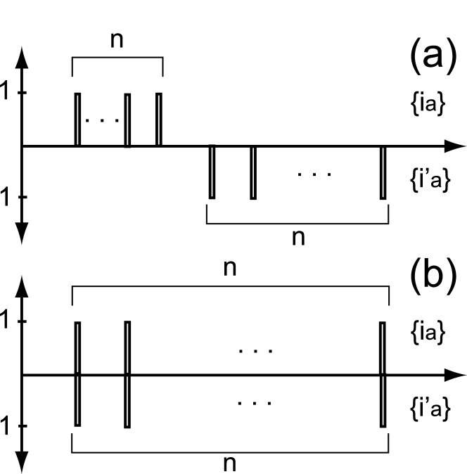
Figure 1: RS saddle-point configurations (33). The horizontal axis represents the index of configurations running from 1 to $2^{N}$. The vertical axis represents the number of each configurations. (a) P1 phase (34) and (b) P2 (35).

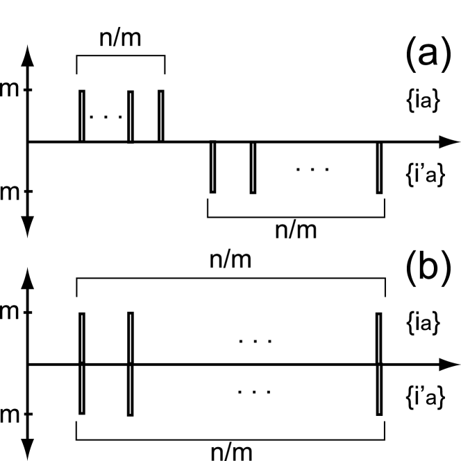
Figure 2: 1RSB saddle-point configurations (47). (a) SG phase with $\tilde{q}=0$ and (b) that with $\tilde{q}\neq 0$.

Next, we treat the 1RSB SG solution which can be expressed in figure 2. We have for $q_{ab}$ and $q^{\prime}_{ab}$

$$\sum_{ab}q_{ab}=\sum_{ab}q^{\prime}_{ab}=mn,$$ (47)

where $m$ is the Parisi breaking parameter. For the configuration in figure 2(a), there is no overlap between $\{i_{a}\}$ and $\{i^{\prime}_{a}\}$ and

$$\tilde{q}_{ab}=0.$$ (48)

For that in figure 2(b), $\tilde{q}_{ab}$ has the 1RSB structure and

$$\sum_{ab}\tilde{q}_{ab}=mn.$$ (49)

Then, for each saddle point,

$$\phi=\left\{\begin{array}[]{ll}\frac{\ln 2}{m}+\frac{m}{4}(\beta_{1}^{2}-\beta_{2}^{2})J^{2}\\ \frac{\ln 2}{2m}+\frac{m}{2}\beta_{1}^{2}J^{2}\end{array}\right..$$ (52)

$m$ is optimized as

$$m=\left\{\begin{array}[]{l}\frac{\beta_{\rm c}}{\sqrt{\beta_{1}^{2}-\beta_{2}^{2}}}\\ \frac{\beta_{\rm c}}{2|\beta_{1}|}\end{array}\right.,$$ (55)

and we obtain

$$\phi=\left\{\begin{array}[]{l}\frac{J^{2}}{2}\beta_{\rm c}\sqrt{\beta_{1}^{2}-\beta_{2}^{2}}\\ \frac{J^{2}}{2}\beta_{\rm c}|\beta_{1}|\end{array}\right..$$ (58)

In both the cases, the entropy is shown to be zero. The former solution is always smaller than the latter one and is discarded.

We summarize the result as

$$\phi=\left\{\begin{array}[]{lll}\frac{J^{2}}{4}(\beta_{1}^{2}-\beta_{2}^{2}+\beta_{\rm c}^{2})&(\beta_{1}^{2}-\beta_{\rm c}^{2}\leq\beta_{2}^{2})&{\rm P1}\\ \frac{J^{2}}{2}\left(\beta_{1}^{2}+\frac{\beta_{\rm c}^{2}}{4}\right)&(|\beta_{1}|\leq\beta_{\rm c}/2)&{\rm P2}\\ \frac{J^{2}}{2}\beta_{\rm c}|\beta_{1}|&&{\rm SG}\end{array}\right..$$ (62)

We compare these solutions to take the maximum value of $\phi$. The condition that P1 is larger than P2 is

$$\beta_{1}^{2}+\beta_{2}^{2}<\frac{\beta_{\rm c}^{2}}{2},$$ (63)

and that P1 is larger than SG is

$$(|\beta_{1}|-\beta_{\rm c})^{2}>\beta_{2}^{2}.$$ (64)

SG is always larger than P2. They are equal when $|\beta_{1}|=\beta_{\rm c}/2$. In conclusion, the phase diagram is obtained as in figure 4.

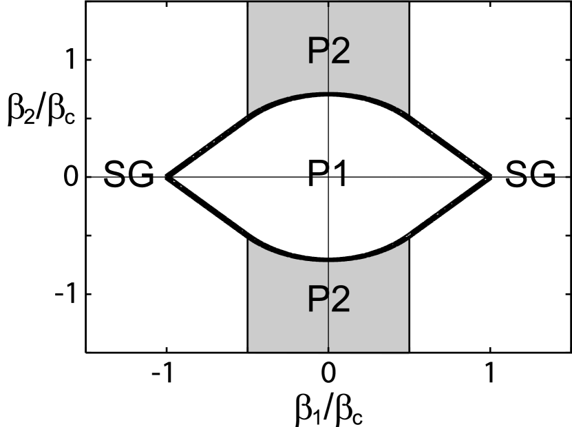
Figure 3: Phase diagram and distribution of partition-function zeros of the REM in the complex-$\beta$ plane. Zeros are distributed in the shaded area and on the bold lines.

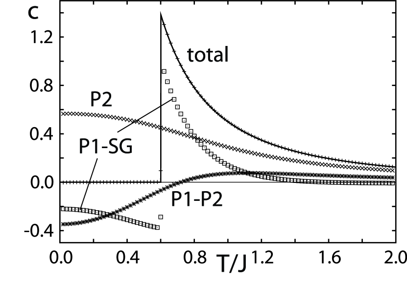
Figure 4: The specific heat calculated from (73). The solid line represents the exact result $c=(J^{2}/2T^{2})\theta(T-T_{\rm c})$ where $T_{\rm c}=1/\beta_{\rm c}$.

4.4 Density of zeros

Now we calculate the density of zeros by using formula (9). The density of zeros in each phase is given by

$$\rho_{\beta}(\beta_{1},\beta_{2})=\left\{\begin{array}[]{ll}0&{\rm P1}\\ J^{2}/2\pi&{\rm P2}\\ 0&{\rm SG}\end{array}\right..$$ (68)

In addition to this, zeros are distributed on phase boundaries where the derivative of the free energy shows a discontinuous change. On the P1-P2 boundary, that is, $\beta_{1}^{2}+\beta_{2}^{2}=\beta_{\rm c}/2$ and $0<|\beta_{1}|/\beta_{\rm c}<1/2$, the density of zeros is calculated as

$$\rho_{\beta}(\beta_{1},\beta_{2}) = \frac{1}{2\pi}\left(\frac{\partial^{2}}{\partial\beta_{1}^{2}}+\frac{\partial^{2}}{\partial\beta_{2}^{2}}\right)\left\{\phi_{\rm P1}\theta(\phi_{\rm P1}-\phi_{\rm P2})+\phi_{\rm P2}\theta(\phi_{\rm P2}-\phi_{\rm P1})\right\}$$ (69)

$$= \frac{J^{2}}{2\pi}\frac{\beta_{\rm c}^{2}}{2}\delta(\beta_{1}^{2}+\beta_{2}^{2}-\beta_{\rm c}^{2}/2),$$ (70)

where $\theta$ is the step function such that $\theta(x)=1$ when $x$ is positive and 0 when negative. In the same way, on the P1-SG boundary $|\beta_{1}|+|\beta_{2}|=\beta_{\rm c}$ and $1/2<|\beta_{1}|/\beta_{\rm c}<1$,

$$\rho_{\beta}(\beta_{1},\beta_{2})=\frac{J^{2}}{2\pi}\beta_{2}\delta(|\beta_{1}|-\beta_{\rm c}+|\beta_{2}|).$$ (71)

On the P2-SG boundary $|\beta_{1}|/\beta_{\rm c}=1/2$ and $1/2<|\beta_{2}|/\beta_{\rm c}$, the boundary distribution of zeros is shown to be zero. We conclude that the density of zeros in the REM is given by

$$\rho_{\rm\beta}(\beta_{1},\beta_{2}) = \frac{J^{2}}{2\pi}\theta(\beta_{\rm c}/2-|\beta_{1}|)\theta(\beta_{1}^{2}+\beta_{2}^{2}-\beta_{\rm c}^{2}/2)$$ (72)

$$+\frac{J^{2}}{2\pi}\frac{\beta_{\rm c}^{2}}{2}\delta(\beta_{1}^{2}+\beta_{2}^{2}-\beta_{\rm c}^{2}/2)\theta(\beta_{\rm c}/2-|\beta_{1}|)$$

$$+\frac{J^{2}}{2\pi}\beta_{2}\delta(|\beta_{1}|+|\beta_{2}|-\beta_{\rm c})\theta(|\beta_{1}|-\beta_{\rm c}/2)\theta(\beta_{\rm c}-|\beta_{1}|).$$

The result coincides with that in [19].

4.5 Discussions

We have re-derived the density of zeros by using the replica method, which allows us to clarify the following properties of the distribution:

• Figures of the distribution of zeros can be viewed as phase diagrams in the complex plane. There are two types of distributions for the density of zeros: two-dimensional distribution within a phase and one-dimensional one at a phase boundary.

• When $\tilde{q}_{ab}=0$, the two configurations $\{i_{a}\}$ and $\{i^{\prime}_{a}\}$ become independent of each other. Then, the average partition function decouples as (16) and $\phi$ is written as a sum $\phi=\phi_{0}(\beta)+\phi_{0}(\beta^{*})$. In this case, the density of state is shown to be zero.

• When $\tilde{q}_{ab}\neq 0$, there are correlations between two configurations $\{i_{a}\}$ and $\{i^{\prime}_{a}\}$. Then, two-dimensional distributions of zeros can be obtained. Since the correlation occurs only when the ensemble average is taken, one can say that the two-dimensional distribution is specific to random systems. In the case of the REM, two configurations are completely identical: $\{i_{a}\}=\{i^{\prime}_{a}\}$ in the P2 and SG phases.

• However, $\tilde{q}_{ab}\neq 0$ is not the sufficient condition for two-dimensional distributions. In the REM, a two-dimensional distribution appears in the P2 phase and not in the SG one. Our result indicates that two-dimensional distributions are not specific to the SG phase. In the SG phase of the REM, the system freezes to its ground state and the entropy goes to zero. In such a frozen phase, zeros do not appear.

• The two-dimensional distribution of zeros in the P2 phase is located far from the real physical axis and near the imaginary axis. On the imaginary axis, the Boltzmann factor is given by $e^{-i\beta_{2}H}$ and can take arbitrary values. Therefore, it is a natural result that zeros appear around the imaginary axis. It is interesting to see that the zeros can appear only when $\beta_{2}>\beta_{\rm c}/\sqrt{2}$ on the imaginary axis. Since $e^{-i\beta_{2}H}$ is nothing but the time evolution operator, the result may be related to dynamical properties of the system.

• The one-dimensional distribution of zeros on the P1-SG boundary meets with the real axis at the angle of $\pi/4$, and the density of zeros is zero at the phase transition point on the real axis. These properties are characteristics of second-order phase transitions [27]. We discuss these properties closely in section 6.

• To understand the role of each zero, we calculate the specific heat from the obtained density of zeros. Using (8), we can write the specific heat as

  $$c=\int dz_{1}dz_{2}\,\rho_{\beta}(z_{1},z_{2})\frac{-\beta^{2}}{(\beta-z)^{2}},$$ (73)

  which allows us to write the function as a sum of contributions from each phase and boundary. The result is plotted in figure 4. The singularity at the transition point comes from the zeros in the P1-P2 boundary. At large temperature, the main contribution comes from the zeros in the P2 phase. In the SG phase lower than the transition point, the contributions from the boundaries give a negative specific heat. All contributions cancel out to give the zero specific heat. As we decrease the temperature, zeros far from the real axis in the P2 phase become more important.

• In section 4.2, we have defined the entropy for complex temperature by using the Legendre transformation. It is not obvious whether we should impose the nonnegative condition to the entropy since the function has not been defined as the number of states. In fact, the condition (45) in the P1 phase has not been used to determine the phase boundary. The results in the P2 and SG phases may be understood the number of states since the entropy is independent of the imaginary part of the temperature. Therefore, although the definition of the entropy in section 4.2 looks like a natural one, we need more discussion for the physical meaning of the entropy.

5 GREM and the full RSB limit

In contrast to a naive expectation that the two-dimensional distribution of zeros is specific to the SG phase, our result shows that zeros are not in the SG phase but in a P phase. The area-distributed domain is not on the real axis and cannot be directly related to the SG phase transition.

The REM is considered the simplest SG model since the SG phase is described by the 1RSB solution and the order parameter only takes either 0 or 1. We want to discuss more complicated situations keeping the advantage of the REM that the analytical calculation is possible. For this purpose, we employ the GREM [23, 24, 25, 26]. This model is a simple generalization of the REM and allows us to analyze higher step RSB solutions easily. We consider the distribution of zeros in the GREM and discuss possible distributions at the full RSB limit.

5.1 Model

The GREM is defined by a hierarchical structure of energy levels. Each energy level is expressed by the sum of $K$ random numbers. To the $\nu$th level of hierarchy with $1\leq\nu\leq K$, we assign random variables $\epsilon_{\nu}(1),\epsilon_{\nu}(2),\cdots,\epsilon_{\nu}(M_{\nu})$. The number of variables $M_{\nu}$ is given by

$$M_{\nu}=(\alpha_{1}\cdots\alpha_{\nu})^{N},$$ (74)

where each $\alpha_{\nu}^{N}$ is an integer with $1<\alpha_{\nu}^{N}<2^{N}$ satisfying

$$M_{K}=(\alpha_{1}\cdots\alpha_{K})^{N}=2^{N}.$$ (75)

For the $\nu$th level of hierarchy, we generate random numbers with Gaussian distribution

$$P_{\nu}(\epsilon_{\nu})=\frac{1}{\sqrt{\pi NJ^{2}a_{\nu}}}\exp\left(-\frac{\epsilon_{\nu}^{2}}{NJ^{2}a_{\nu}}\right),$$ (76)

where $a_{\nu}>0$ satisfies

$$\sum_{\nu=1}^{K}a_{\nu}=1.$$ (77)

From the random numbers generated as above, we construct $2^{N}$-random numbers as

$$E_{i}=\sum_{\nu=1}^{K}\epsilon_{\nu}(\lfloor(i-1)M_{\nu}/2^{N}\rfloor+1),$$ (78)

where $i=1,2,\cdots,2^{N}$ and $\lfloor x\rfloor$ is the floor function which indicates the largest integer not exceeding $x$.

The GREM is defined as a system with energy levels (78). By choosing parameters in an appropriate way, we can find multiple phase transitions. We define

$$T_{\nu}=\frac{J}{2}\sqrt{\frac{a_{\nu}}{\ln\alpha_{\nu}}},$$ (79)

where $\nu=1,2,\cdots,K$. If $T_{1}>T_{2}>\cdots>T_{K}$, phase transitions occur at these temperatures.

In the replica analysis of this model, the SG order parameter $q_{ab}^{(\nu)}$ is defined at each hierarchy $\nu$ [26]. At $T>T_{1}$, all the parameters are given by the P solution $q_{ab}^{(\nu)}=\delta_{ab}$. At $T=T_{\nu}$, $q_{ab}^{(\nu)}$ turns into the 1RSB solution and the degrees of freedom in the $\nu$th hierarchy fall into the ground state. For example, when we consider the $K=2$ case, the system goes into the P-P, SG-P and SG-SG phases as the temperature is decreased. It is understood from the complexity analysis that the SG-P phase is identified as the 1RSB state and the SG-SG phase as the two-step RSB one.

5.2 Distribution of zeros

It is a straightforward task to apply the calculation of zeros in the previous section to the GREM. We consider two hierarchy ($K=2$) system and choose parameters so that the relation $T_{1}>T_{2}$ is satisfied. We calculate $\phi=[\ln|Z|]/N$ in each phase. Following the calculation in [26], we find

$$\phi=\left\{\begin{array}[]{ll}\ln 2+\frac{1}{4}(\beta_{1}^{2}-\beta_{2}^{2})J^{2}&{\rm P1-P1}\\ \frac{1}{2}\ln\alpha_{1}+\frac{a_{1}}{2}\beta_{1}^{2}J^{2}+\ln\alpha_{2}+\frac{a_{2}}{4}(\beta_{1}^{2}-\beta_{2}^{2})J^{2}&{\rm P2-P1}\\ \frac{1}{2}\ln 2+\frac{1}{2}\beta_{1}^{2}J^{2}&{\rm P2-P2}\\ \beta_{1}J\sqrt{a_{1}\ln\alpha_{1}}+\ln\alpha_{2}+\frac{a_{2}}{4}(\beta_{1}^{2}-\beta_{2}^{2})J^{2}&{\rm SG-P1}\\ \beta_{1}J\sqrt{a_{1}\ln\alpha_{1}}+\frac{1}{2}\ln\alpha_{2}+\frac{a_{2}}{2}\beta_{1}^{2}J^{2}&{\rm SG-P2}\\ \beta_{1}J\left(\sqrt{a_{1}\ln\alpha_{1}}+\sqrt{a_{2}\ln\alpha_{2}}\right)&{\rm SG-SG}\end{array}\right.,$$ (86)

which is easily understood as a straightforward extension of the result in the previous section to the two-hierarchy case. Then, comparing these solutions, we obtain the phase diagram and distribution of zeros in figure 6. Zeros are distributed in the shaded regions and on the bold lines of the figure. We have two phase transitions at $T=T_{1,2}$ and correspondingly, two lines of zeros touch the real axis. Still, the shaded regions are far from the real axis and are not related to the SG transition.

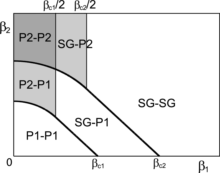
Figure 5: Phase diagram and distribution of zeros of the GREM with two hierarchies in the complex-$\beta$ plane. The plot is only in the first quadrant. Zeros are distributed in the shaded regions and on the bold lines.

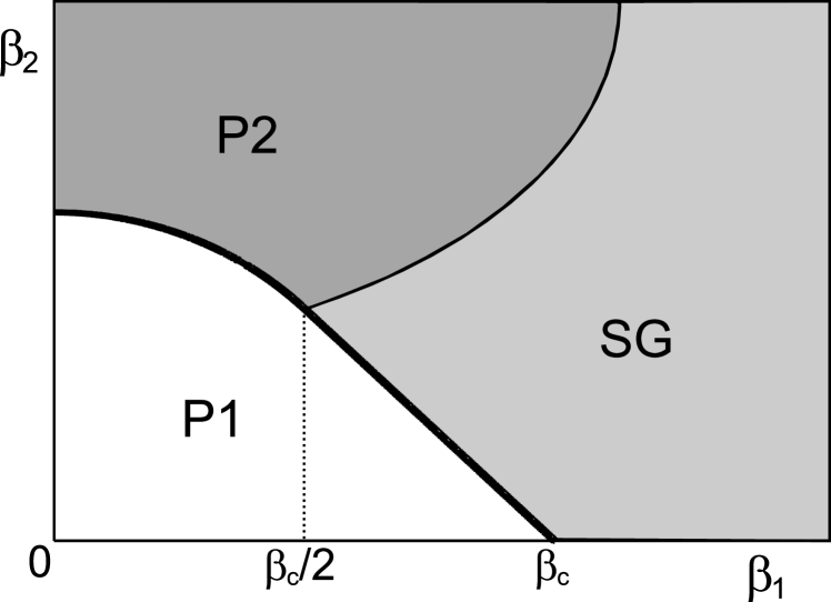
Figure 6: A continuous limit $K\to\infty$ of the GREM. Critical temperatures change continuously between $T_{1}=1/\beta_{\rm c}$ and $T_{K}=0$.

An interesting result is obtained when we consider the continuum limit of hierarchy. Then, the critical temperatures become continuous between $T_{1}$ and $T_{K}$ and the SG phase can be understood as the full step RSB state. We can find a similar, but different, behavior as the Sherrington-Kirkpatrick model [28] which also has the full RSB SG phase. In the GREM, the continuum limit is not unique and depends on the choice of parameters [24]. We show a typical example with $T_{K}=0$ in figure 6. We see that the line distributions at phase boundaries are accumulated to become area distributions. In the P2 phase of the figure, the original area distributions and accumulated lines overlap with each other and cannot be distinguished. The area distribution in the SG phase comes in contact with the real axis, which is consistent with the picture that phase transitions occur continuously in the full RSB SG phase. Actually, a similar numerical result has been obtained for a system on the Bethe lattice [12]. Our result in the GREM shows that distributions of zeros in SG systems with a full RSB state are more complicated than those in the REM.

6 Ferromagnetic interaction and first order transition

In the previous sections, we have studied the REM. This model is described by a random distribution of energy levels and the spin degrees of freedom do not appear at all. Therefore, in order to extend our method to other spin models, it is necessary to treat the spin Hamiltonian. To achieve this, we treat the $p$-spin model in (12). At the same time, to motivate the use of the spin representation, we treat the positive regular interaction $J_{0}$ whose effect is incorporated to the probability distribution of $J_{i_{1}\cdots i_{p}}$ as

$${\rm P}_{\rm J}(J_{i_{1}\cdots i_{p}})=\sqrt{\frac{N^{p-1}}{\pi p!J^{2}}}\exp\left\{-\frac{N^{p-1}}{p!J^{2}}\left(J_{i_{1}i_{2}\cdots i_{p}}-\frac{p!J_{0}}{N^{p-1}}\right)^{2}\right\}.$$ (87)

At large $J_{0}$, the system is in the ferromagnetic (F) phase which is characterized by the magnetization $m=\sum_{i}\langle S_{i}\rangle/N$ where $\langle\,\rangle$ denotes the thermal average. At the REM limit $p\to\infty$, the model can be solved exactly, and the phase diagram in the $J_{0}-T$ plane is obtained as in figure 8. The phase boundary between the SG and F phases is given by $J_{0}=J_{0{\rm c}}=J\sqrt{\ln 2}$ and that between the P and F phases by

$$T=\frac{J^{2}}{2}\frac{1}{J_{0}-\sqrt{J_{0}^{2}-J^{2}\ln 2}}.$$ (88)

The transition between the P and F phases is of first order and the entropy shows a discontinuous change. Therefore, by treating this model we can study both the spin representation and the first-order phase transition in our replica formulation.

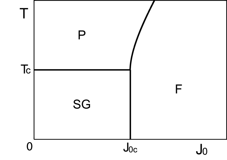
Figure 7: Phase diagram of the REM with the F interaction $J_{0}$. The P-F transition is of first order and the others of second order.

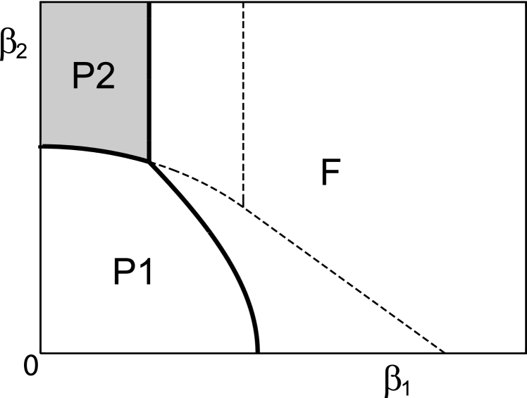
Figure 8: Phase diagram and distribution of zeros of the REM at $J_{0}>J_{0{\rm c}}=J\sqrt{\ln 2}$. The dashed lines are the phase boundaries at $J_{0}<J_{0\rm c}$.

Following the standard method to calculate $[Z^{n}]$ [1, 2, 3, 18], we can treat $[|Z|^{2n}]$ in a similar way. Since the replica space is doubled to the complex conjugate space, we have two kinds of spin variables $\{S_{i}^{a}\}$ and $\{S_{i}^{{}^{\prime}a}\}$. Correspondingly, the SG order parameters are defined as $q_{ab}\sim\sum_{i}\langle S_{i}^{a}S_{i}^{b}\rangle/N$, $q^{\prime}_{ab}\sim\sum_{i}\langle S_{i}^{{}^{\prime}a}S_{i}^{{}^{\prime}b}\rangle/N$ and $\tilde{q}_{ab}\sim\sum_{i}\langle S_{i}^{a}S_{i}^{{}^{\prime}b}\rangle/N$. Since we treat the F phase, we also have the magnetization $m_{a}\sim\sum_{i}\langle S_{i}^{a}\rangle/N$ and $m^{\prime}_{a}\sim\sum_{i}\langle S_{i}^{{}^{\prime}a}\rangle/N$. By using these variables, we can write

$$[|Z|^{2n}] = \exp\left\{-N\frac{p-1}{2}\beta^{2}J^{2}\sum_{a>b}(q_{ab})^{p}-N\frac{p-1}{2}\beta^{*2}J^{2}\sum_{a>b}(q^{\prime}_{ab})^{p}\right.$$ (89)

$$-N\frac{p-1}{2}|\beta|^{2}J^{2}\sum_{a>b}(\tilde{q}_{ab})^{p}+\frac{Nn\beta^{2}J^{2}}{4}+\frac{Nn\beta^{*2}J^{2}}{4}$$

$$-N(p-1)\beta J_{0}\sum_{a}(m_{a})^{p}-N(p-1)\beta^{*}J_{0}\sum_{a}(m^{\prime}_{a})^{p}$$

$$+N\ln\Tr\exp\left(\beta^{2}J^{2}\sum_{a>b}\hat{q}_{ab}S_{a}S_{b}+\beta^{*2}J^{2}\sum_{a>b}\hat{q}^{\prime}_{ab}S^{\prime}_{a}S^{\prime}_{b}\right.$$

$$\left.\left.+|\beta|^{2}J^{2}\sum_{a,b}\hat{\tilde{q}}_{ab}S_{a}S^{\prime}_{b}+2\beta J_{0}\sum_{a}\hat{m}_{a}S_{a}+2\beta^{*}J_{0}\sum_{a}\hat{m}^{\prime}_{a}S^{\prime}_{a}\right)\right\},$$

where variables with the hat symbol are related to those without hat as

$$\hat{q}_{ab}=\frac{p}{2}(q_{ab})^{p-1}.$$ (90)

The order parameters are obtained from the saddle-point equations. At $p\to\infty$, the equations are easily solved since the order parameters take either 0 or 1. The P1, P2 and SG phases without the magnetization are calculated in the same way as the previous case and (62) is obtained. In the F phase given by $m_{a}=m^{\prime}_{a}=1$, all spins are aligned to the same direction and we find a simple expression

$$\phi=\beta_{1}J_{0}.$$ (91)

Comparing $\phi$ in each phase, we can write the phase diagram and the distribution of zeros in the complex $\beta$ plane. When $J_{0}<J_{0{\rm c}}$, the F phase solution is irrelevant and we have the phase diagram in figure 4. The result at $J_{0}>J_{0{\rm c}}$ is shown in figure 8. The phase boundary between the P1 and F phases is given by

$$\beta_{2}J=\sqrt{\beta_{1}^{2}J^{2}-4\beta_{1}J_{0}+4\ln 2}$$ (92)

and that between the P2 and F phases by

$$\beta_{1}J^{2}=J_{0}-\sqrt{J_{0}^{2}-J^{2}\ln 2}.$$ (93)

The zeros are distributed in the P2 phase and on all the phase boundaries.

Comparing figures 4 and 8, we can see the difference between the second- and first-order phase transitions. The general consideration shows that there is a relation between the order of the phase transition and the distributions of zeros on the real axis [27]. In the second-order transition, the line distribution meets with the real axis with the angle of $\pi/4$, and the density of zeros goes to zero on the real axis. In contrast, for the first-order transition, the angle between the line and the real axis is $\pi/2$ and the density is finite on the real axis. Our results support these expectations. On the real axis, the density of zeros is given by

$$\rho_{\beta}(\beta_{1},\beta_{2}=0) = \frac{J^{2}}{2\pi}\sqrt{J_{0}^{2}-J^{2}\ln 2}\ \theta(J_{0}-J\sqrt{\ln 2})$$ (94)

$$\times\delta\left(\beta_{1}J^{2}-2(J_{0}-\sqrt{J_{0}^{2}-J^{2}\ln 2})\right).$$

It is also known from the general argument that the density at the transition point is directly related to the discontinuous energy change $\Delta\epsilon$. In the present case, it is obtained as $\Delta\epsilon=\epsilon_{\rm P}-\epsilon_{\rm F}=\sqrt{J_{0}^{2}-J^{2}\ln 2}$. We see that the same factor appears in (94).

7 Lee-Yang zeros of the REM

Up to here we have discussed the Fisher zeros in the REM. In this section, we treat the Lee-Yang zeros in the same model. While the analysis of systems with complex temperature clarifies the system’s thermodynamic properties such as the entropy and specific heat, that with complex magnetic field is useful to understand the magnetic properties such as the magnetization and susceptibility.

The analysis of the Fisher zeros using the replica method goes along the same line as that of the Lee-Yang zeros in the previous sections. To apply the magnetic field, we consider two possible patterns: longitudinal and transverse magnetic fields. The density of zeros in the complex longitudinal field has been studied in [21, 22]. The method used there is very similar to the original analysis of the Fisher zeros in the REM [19]. We re-derive the result by using the replica method. Also, we treat the system with a transverse field, which allows us to study the quantum fluctuation effect.

7.1 Longitudinal magnetic field

We use the energy representation of the REM in (10) and (11). Then, the magnetic field $h$ is incorporated to the partition function as

$$Z=\sum_{M}e^{\beta hM}\sum_{i=1}^{N(M)}e^{-\beta E_{i}(M)},$$ (95)

where $M$ represents the “magnetization” and takes

$$M_{k}=-(N-2k),$$ (96)

with $k=0,1,\cdots,N$. For a given $M_{k}$, the number of the sum $N(M_{k})$ is equal to $N!/k!(N-k)!$. The partition function is written as

$$Z=e^{-N\beta h}\sum_{k=0}^{N}y^{k}\sum_{i=1}^{N(M_{k})}e^{-\beta E_{ki}},$$ (97)

where $y=e^{2\beta h}$ and $E_{ki}$ is a random variable taken from (11). Thus, the partition function is a polynomial of the $N$th degree in $y$ and the density of zeros is obtained from (6).

The REM with real $h$ has been treated in [16, 17] and the phase diagram is depicted in figure 10. The P and SG phases are separated by the critical temperature $T_{\rm c}(h)=1/\beta_{\rm c}(h)$ defined by

$$\frac{\beta_{\rm c}^{2}(h)J^{2}}{4}=\ln(1+e^{2\beta_{\rm c}(h)h})-\frac{2\beta_{\rm c}(h)h}{1+e^{-2\beta_{\rm c}(h)h}}.$$ (98)

As in the previous cases, this transition is also caused by the entropy crisis which means that the entropy goes to zero in the SG phase.

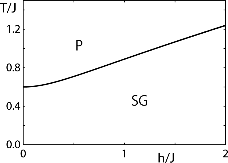
Figure 9: Phase diagram of the REM in the $h-T$ plane. The P-SG transition is of second order.

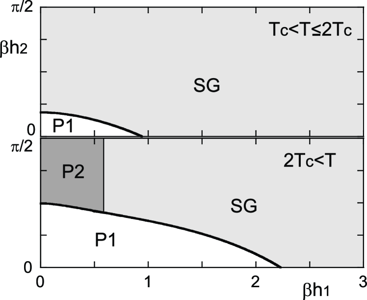
Figure 10: Phase diagram and distribution of zeros of the REM in the complex-$h$ plane. The upper figure is for $T_{\rm c}<T\leq 2T_{\rm c}$ and lower for $2T_{\rm c}<T$. For $T\leq T_{\rm c}$, all domain belongs to the SG phase.

When $h$ is a complex number, the P1, P2 and SG phases appear in the phase diagram. $|Z|^{2n}$ is written as

$$|Z|^{2n} = e^{-2Nn\beta h_{1}}\sum_{\{k_{a},i_{a}\}}\sum_{\{k^{\prime}_{a},i_{a}^{\prime}\}}(y)^{\sum_{k=0}^{N}kn_{k}(\{k_{a}\})}(y^{*})^{\sum_{k=0}^{N}kn^{\prime}_{k}(\{k^{\prime}_{a}\})}$$ (99)

$$\times\exp\left\{-\beta\sum_{k=0}^{N}\sum_{i=1}^{N(M_{k})}\left(n_{ki}(\{k_{a},i_{a}\})+n^{\prime}_{ki}(\{k^{\prime}_{a},i^{\prime}_{a}\})\right)E_{ki}\right\},$$

where

$$n_{ki}(\{k_{a},i_{a}\})=\sum_{a=1}^{n}\delta_{k_{a}k}\delta_{i_{a}i},$$ (100)

$$n_{k}(\{k_{a}\})=\sum_{a=1}^{n}\delta_{k_{a}k}.$$ (101)

Each $k_{a}$ takes $0,1,\cdots,N$ and $i_{a}$ takes $1,2,\cdots,N(M_{k_{a}})$. Taking the average, we obtain

$$[|Z]^{2n} = e^{-2Nn\beta h_{1}}\sum_{\{k_{a},i_{a}\}}\sum_{\{k^{\prime}_{a},i_{a}^{\prime}\}}(y)^{\sum_{k=0}^{N}kn_{k}(\{k_{a}\})}(y^{*})^{\sum_{k=0}^{N}kn^{\prime}_{k}(\{k^{\prime}_{a}\})}$$ (102)

$$\times\exp\left\{\frac{N\beta^{2}J^{2}}{4}\sum_{a,b=1}^{n}\left(q_{ab}+q^{\prime}_{ab}+2\tilde{q}_{ab}\right)\right\},$$

where the order parameters are defined as

$$q_{ab}=\delta_{k_{a}k_{b}}\delta_{i_{a}i_{b}},$$ (103)

$$q^{\prime}_{ab}=\delta_{k_{a}k_{b}}\delta_{i^{\prime}_{a}i^{\prime}_{b}},$$ (104)

$$\tilde{q}_{ab}=\delta_{k_{a}k_{b}}\delta_{i_{a}i^{\prime}_{b}}.$$ (105)

As we mentioned above, we have three phases.

• P1.

  The simplest solution is given by $q_{ab}=q_{ab}^{\prime}=\delta_{ab}$ and $\tilde{q}_{ab}=0$. We have for $\phi=[\ln|Z|]/N$

  $$\phi_{\rm P1}=-\beta h_{1}+\frac{\beta^{2}J^{2}}{4}+\frac{1}{2}\ln(1+e^{2\beta h})+\frac{1}{2}\ln(1+e^{2\beta h^{*}}).$$ (106)

  This is a simple extension of the usual P phase result for real $h$ to the case of complex $h$.

• P2.

  The second simplest case is specific to the complex parameters: $q_{ab}=q_{ab}^{\prime}=\tilde{q}_{ab}=\delta_{ab}$. Then, we have the P2 phase result

  $$\phi_{\rm P2}=-\beta h_{1}+\frac{\beta^{2}J^{2}}{2}+\frac{1}{2}\ln(1+e^{4\beta h_{1}}).$$ (107)

  This is valid at $\beta\leq\tilde{\beta}_{\rm c}(h_{1})=\beta_{\rm c}(h_{1})/2$ where the entropy is nonnegative.

• SG.

  When the temperature is lower than $1/\tilde{\beta}_{\rm c}(h_{1})$, the system freezes to the SG phase. The order parameters are given by (47) and (49). Then,

  $$\phi_{\rm SG}=-\beta h_{1}+\frac{\beta\tilde{\beta}_{\rm c}(h_{1})J^{2}}{2}+\frac{\beta}{2\tilde{\beta}_{\rm c}(h_{1})}\ln(1+e^{4\tilde{\beta}_{\rm c}(h_{1})h_{1}}).$$ (108)

Comparing these results, we can draw the phase diagram in the complex-$h$ plane as figure 10 . Zeros can appear in the P2 and SG phases, and the P1-P2 and P1-SG boundaries. The result is completely the same as that in the previous study obtained by a different method [21].

It is interesting to see that the density of zeros in the SG phase is nonzero as

$$\rho_{h}(h_{1},h_{2})=\beta\tilde{\beta}_{\rm c}(h_{1})\frac{1-\tanh^{2}(2\tilde{\beta}_{\rm c}(h_{1})h_{1})}{1+2(h_{1}^{2}/J^{2})(1-\tanh^{2}(2\tilde{\beta}_{\rm c}(h_{1})h_{1}))},$$ (109)

in contrast to the case of the Fisher zeros where the zeros do not appear in the SG phase. In the present case, although the entropy is zero in the SG phase, the critical temperature depends on the magnetic field and the value of the free energy depends sensitively on the field. As a result, the density of zeros gives a finite value. But we note that the function (109) decays exponentially in $h_{1}$ and takes considerably small values, which mean that zeros very rarely exist in the SG phase.

Another interesting point is that the P2 phase appears at $T\geq 2T_{\rm c}=1/\tilde{\beta}_{\rm c}(0)$. This property is the same as that of the Fisher zeros (see figures 4, 6 and 6). At present, the reason why $2T_{\rm c}$ plays a special role is not clear. It may be interesting to see whether this property is specific to the REM or not.

7.2 Transverse magnetic field

Then, we consider the REM in a transverse field [29]. The Hamiltonian is given by

$$H=-\sum_{i_{1}<\cdots<i_{p}}J_{i_{1}\cdots i_{p}}\sigma_{i_{1}}^{z}\cdots\sigma_{i_{p}}^{z}-\Gamma\sum_{i=1}^{N}\sigma_{i}^{x},$$ (110)

where $\sigma_{z}$ and $\sigma_{x}$ are the Pauli matrices. Since two terms in the right-hand side of the equation do not commute with each other, the system must be treated quantum mechanically. At the REM limit $p\to\infty$, this model can be solved exactly and the phase diagram is given by figure 12. We have two kinds of P phases: the classical P (CP) and quantum P (QP) phases. The CP phase is the same as the P phase in the classical REM and spins are directed along the $z$-direction randomly. On the other hand, in the QP phase, spins are aligned with the transverse-field direction.

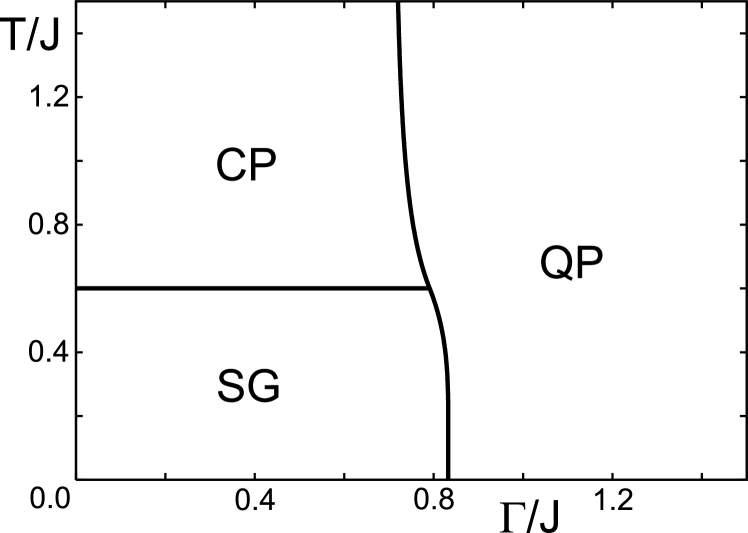
Figure 11: Phase diagram of the REM in a transverse magnetic field $\Gamma$. The CP-QP and SG-QP transitions are of first order.

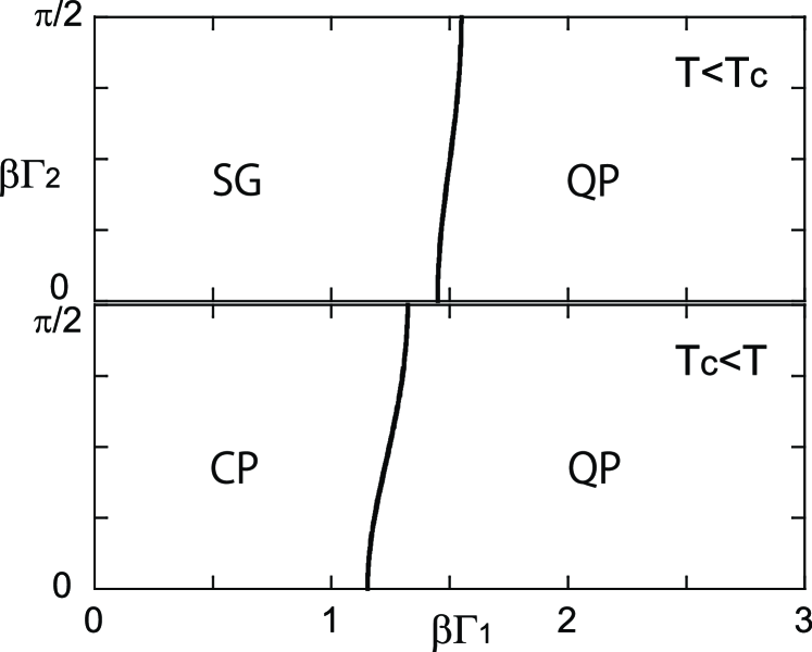
Figure 12: Phase diagram and distribution of zeros of the REM in the complex-$\Gamma$ plane. The upper figure is for $T<T_{\rm c}=J/2\sqrt{\ln 2}$ and lower for $T_{\rm c}<T$.

The average replicated partition function is written in terms of order parameters $\chi_{a}(\tau,\tau^{\prime})\sim\sum_{i}\langle S_{zi}^{a}(\tau)S_{zi}^{a}(\tau^{\prime})\rangle/N$ and $q_{ab}(\tau,\tau^{\prime})\sim\sum_{i}\langle S_{zi}^{a}(\tau)S_{zi}^{b}(\tau^{\prime})\rangle/N$ where $a\neq b$. Since we are treating the quantum system, the trace is defined by the imaginary time path integral with some measure [30], and the spin variable $\mbox{\boldmath$S$}_{i}^{a}$ depends on the time $\tau$. The order parameter $\chi_{a}$ with $q_{ab}\leq\chi_{a}\leq 1$ characterizes quantum effects since $\chi_{a}=1$ in the classical system.

When $\Gamma$ is real, the model is solved by the 1RSB and static ansatz. We expect that the same ansatz can be applied to the case of complex $\Gamma$. Proceeding in a similar way as the previous cases, we have

$$[|Z|^{2n}] = \exp\left\{-\frac{Nn\beta^{2}J^{2}}{4}(p-1)\Bigl{(}\chi^{p}-(1-m)q^{p}\Bigr{)}\right.$$ (111)

$$\qquad-\frac{Nn\beta^{*2}J^{2}}{4}(p-1)\Bigl{(}\chi^{\prime p}-(1-m)q^{\prime p}\Bigr{)}$$

$$\left.\qquad-\frac{Nn|\beta|^{2}J^{2}}{2}(p-1)\Bigl{(}\tilde{\chi}^{p}-(1-m)\tilde{q}^{p}\Bigr{)}+N\ln\Tr e^{L}\right\},$$

$$\Tr e^{L} = \Tr\exp\left\{\frac{\beta^{2}J^{2}}{2}\left(\hat{\chi}-\hat{q}\right)\sum_{a=1}^{n}(\hat{S}_{z}^{a})^{2}+\frac{\beta^{2}J^{2}}{2}\hat{q}\sum_{\rm B}^{n/m}\left(\sum_{a\in B}^{m}\hat{S}_{z}^{a}\right)^{2}\right.$$ (112)

$$+\frac{\beta^{2}J^{2}}{2}\left(\hat{\chi}^{\prime}-\hat{q}^{\prime}\right)\sum_{a=1}^{n}(\hat{S}_{z}^{{}^{\prime}a})^{2}+\frac{\beta^{2}J^{2}}{2}\hat{q}^{\prime}\sum_{\rm B}^{n/m^{\prime}}\left(\sum_{a\in B}^{m^{\prime}}\hat{S}_{z}^{{}^{\prime}a}\right)^{2}$$

$$+\beta^{2}J^{2}(\hat{\tilde{\chi}}-\hat{\tilde{q}})\sum_{a=1}^{n}\hat{S}_{z}^{a}\hat{S}_{z}^{{}^{\prime}a}+\frac{\beta^{2}J^{2}}{2}\hat{\tilde{q}}\sum_{\rm B}^{n/m}\left(\sum_{a\in B}^{m}\hat{S}_{z}^{a}\right)\left(\sum_{a\in B}^{m}\hat{S}_{z}^{{}^{\prime}a}\right)$$

$$\left.+\beta\Gamma\sum_{a=1}^{n}\hat{S}_{x}^{a}+\beta\Gamma^{*}\sum_{a=1}^{n}\hat{S}_{x}^{{}^{\prime}a}\right\},$$

where $\hat{S}^{a}_{z}=\int_{0}^{\beta}d\tau\,S^{a}_{z}(\tau)/\beta$ and the order parameters with the hat symbol are defined in the same way as in (90). Possible saddle-point solutions are given as follows.

• CP.

  $\chi=\chi^{\prime}=1$ and the other parameters are set to zero. In this case the quantum effect is irrelevant, and we have the CP result

  $$\phi_{\rm CP}=\frac{\beta^{2}J^{2}}{4}+\ln 2.$$ (113)

  From the nonnegative condition of the entropy, this solution is shown to be effective at $T>T_{\rm c}=J/2\sqrt{\ln 2}$.

• QP.

  When the transverse field is strong enough so that the effect of interaction is negligible, there is not any order in the $z$-direction. Then, all the order parameters are neglected, and we obtain

  $$\phi_{\rm QP}=\frac{1}{2}\ln(e^{\beta\Gamma}+e^{-\beta\Gamma})+\frac{1}{2}\ln(e^{\beta\Gamma^{*}}+e^{-\beta\Gamma^{*}}).$$ (114)

• SG.

  At low temperatures the system freezes to the ground state. In this case, $\chi=q=1$, and we have the standard 1RSB result

  $$\phi_{\rm SG}=\beta J\sqrt{\ln 2}.$$ (115)

We see that any phase which is specific to the complex parameters does not appear. For example, we can examine the CP2 phase defined by $\chi=\chi^{\prime}=\tilde{\chi}=1$ and $q=q^{\prime}=\tilde{q}=0$. Then, we have

$$\phi_{\rm CP2}=\frac{\beta^{2}J^{2}}{2}+\frac{1}{2}\ln 2.$$ (116)

This solution is valid at $T>2T_{\rm c}=J/\sqrt{\ln 2}$. In this region, $\phi_{\rm CP2}$ is smaller than $\phi_{\rm CP}$. Therefore, we can conclude that the CP2 phase is irrelevant. In the same way, we can also show that the “QP2” phase does not appear.

The phase diagram is shown in figure 12. We do not have any two-dimensional distribution of zeros and zeros are distributed on the phase boundary. The phase boundaries between CP/SG and QP phases are determined by

$$\cosh(2\beta\Gamma_{1})+\cos(2\beta\Gamma_{2})=\frac{1}{2}e^{2\phi_{\rm CP/SG}}.$$ (117)

Their transitions are of first order, and we see that the general argument, the lines of zeros are vertical to the real axis, also holds in this quantum case.

8 Conclusions

We have discussed the partition-function zeros in random energy models by using a new replica method. We re-derived previously obtained results and obtained several new results on the distribution of zeros of random systems. Our method is very general and systematic and can in principle be applied to any spin model.

We find that the two-dimensional distribution of zeros is characterized by the order parameter $\tilde{q}_{ab}$ which connects configurations between the original and complex conjugated spaces. In the REM with complex temperature, the area-distributed phase is paramagnetic rather than a SG phase. It does not appear at real $\beta$, but the physical quantities of the real system are affected by this phase any way as we have demonstrated for the specific heat.

We also find differences between first- and second-order transitions. We showed that the general argument discussed in [27] holds even for random systems. Since our result is not a rigorous proof of the statement, it would be interesting to find a counterexample in other models.

In contrast to previous numerical analyses of finite-dimensional SG systems, we find in the REM that the area distribution of zeros does not approach the real axis. This is because the REM is an oversimplified SG model. In the REM, the SG phase is described by the 1RSB ansatz and the entropy goes to zero in the SG phase. These properties do not hold in general. In fact, the analysis of the GREM at the continuum limit shows a more complicated behavior. Therefore, the next thing to do will be to apply our method to other mean-field models such as the Sherrington-Kirkpatrick model [28] and the spherical model [31, 32]. The formulation is the same as in the present case, and we can utilize the expression (89) for general $p$-spin systems. The difference arises when we solve the saddle-point equation. The SG order parameters take values between 0 and 1, and possibly complex values. Such a situation does not exist for the REM, and we need a careful analysis, which will be done in a future work.

Another point to be discussed is to see how the thermodynamic limit is obtained by taking the size of the system to infinity. We want to know how the zeros approach the real axis of the complex plane. Our analysis is based on the saddle-point method and is valid only in the thermodynamic limit. Therefore, we need to take a different way. Recently, the spherical model has been solved for arbitrary system size [33]. If the method developed there is also useful for systems with complex parameters, we can study finite size effects for the distribution of zeros. It will be an interesting task to solve that problem in future works.

References

References

- [1] Mézard M, Parisi G and Virasoro M A 1987 Spin Glass Theory and Beyond (Singapore: World Scientific)
- [2] Nishimori H 2001 Statistical Physics of Spin Glasses and Information Processing: An Introduction (Oxford: Oxford University Press)
- [3] Mézard M and Montanari A 2009 Information, Physics, and Computation (Oxford: Oxford University Press)
- [4] Yang C N and Lee T D 1952 Phys. Rev.87 404
- [5] Lee T D and Yang C N 1952 Phys. Rev.87 410
- [6] Nishimori H and Ortiz G 2011 Elements of Phase Transitions and Critical Phenomena (Oxford: Oxford University Press)
- [7] Fisher M E 1964 The Nature of Critical Points (Lectures in Theoretical Physics vol 7C) (Boulder: University of Colorado Press)
- [8] Ozeki Y and Nishimori H 1988 J. Phys. Soc. Japan57 1087
- [9] Bhanot G and Lacki J 1993 J. Stat. Phys. 71 259
- [10] Damgaard P H and Lacki J 1995 Int. J. Mod. Phys. C 6 819
- [11] Matsuda Y, Nishimori H and Hukushima K 2008 J. Phys. A: Math. Theor. 41 324012
- [12] Matsuda Y, Müller M, Nishimori H, Obuchi T and Scardicchio A 2010 J. Phys. A: Math. Theor. 43 285002
- [13] Parisi G 1980 J. Phys. A: Math. Gen.13 L115
- [14] Parisi G 1980 J. Phys. A: Math. Gen.13 1101
- [15] Parisi G 1980 J. Phys. A: Math. Gen.13 1887
- [16] Derrida B 1980 Phys. Rev. Lett.45 79
- [17] Derrida B 1981 Phys. Rev.B 24 2613
- [18] Gross D J and Mézard M 1984 Nucl. Phys.B 240 431
- [19] Derrida B 1991 Physica A 177 31
- [20] Moukarzel C and Parga N 1991 Physica A 177 24
- [21] Moukarzel C and Parga N 1992 J. Phys. I France 2 251
- [22] Moukarzel C and Parga N 1992 Physica A 185 305
- [23] Derrida B 1985 J. Physique Lett. 46 L401
- [24] Derrida B and Gardner E 1986 J. Phys. C: Solid State Phys. 19 2253
- [25] Derrida B and Gardner E 1986 J. Phys. C: Solid State Phys. 19 5783
- [26] Obuchi T, Takahashi K and Takeda K 2010 J. Phys. A: Math. Theor. 43 485004
- [27] Abe R 1967 Prog. Theor. Phys. 37 1070
- [28] Sherrington D and Kirkpatrick S 1975 Phys. Rev. Lett.35 1792
- [29] Goldschmidt Y Y 1990 Phys. Rev.B 41 4858
- [30] Takahashi K 2007 Phys. Rev.B 76 184422
- [31] Kosterlitz J M, Thouless D J and Jones R C 1976 Phys. Rev. Lett.36 1217
- [32] Crisanti A and Sommers H-J 1992 Z. Phys.B 87 341
- [33] Akhanjee S and Rudnick J 2010 Phys. Rev. Lett.105 047206