HAT-P-27b: A Hot Jupiter Transiting a G Star on a 3 day orbit

Abstract

We report the discovery of HAT-P-27b, an exoplanet transiting the moderately bright G8 dwarf star GSC 0333-00351 ($V=12.214$). The orbital period is $3.039586\pm 0.000012$ d, the reference epoch of transit is $2455186.01879\pm 0.00054$ (BJD), and the transit duration is $0.0705\pm 0.0019$ d. The host star with its effective temperature $5300\pm 90$ K is somewhat cooler than the Sun, and is more metal-rich with a metallicity of $+0.29\pm 0.10$. Its mass is $0.94\pm 0.04$ $M_{\sun}$ and radius is $0.90_{-0.04}^{+0.05}$ $R_{\sun}$. For the planetary companion we determine a mass of $0.660\pm 0.033$ $M_{\rm J}$ and radius of $1.038_{-0.058}^{+0.077}$ $R_{\rm J}$. For the 30 known transiting exoplanets between 0.3 $M_{\rm J}$ and 0.8 $M_{\rm J}$, a negative correlation between host star metallicity and planetary radius, and an additional dependence of planetary radius on equilibrium temperature are confirmed at a high level of statistical significance.

1. Introduction

Studying exoplanets is vital for understanding our own Solar System, particularly its formation. The sample of more than 500 confirmed exoplanets so far enables us, for example, to test accretion and migration theories (Ida & Lin, 2008), study tidal interactions (Mardling, 2007), examine atmospheric structures (Fortney, 2010), and investigate correlations between the existence of planetary companions and the host star’s metallicity (Ida & Lin, 2004), and between the mass of close-in planets and the spectral type of their host star (Ida & Lin, 2005).

Among these planets, transiting ones are of special significance, because the transit parameters yield planetary mass and radius estimates. They also provide a means to determine some of the stellar parameters more accurately than is possible with spectroscopy alone, such as the stellar surface gravity. The more than 100 transiting exoplanets confirmed to date provide a sample large enough to draw meaningful conclusions about the planetary parameters that could not be determined by radial velocity (RV) data alone; for example, the correlation between stellar chromospheric activity and planetary surface gravity (Hartman, 2010), or the correlation of planetary parameters with host star metallicity and planetary equilibrium temperature, as described in Section 4.

The Hungarian-made Automated Telescope Network (HATNet; Bakos et al., 2011) is a system of fully automated wide-field small telescopes designed to detect the small photometric dips when exoplanets transit their host stars. Since 2006, HATNet has announced and published 26 planetary systems with 28 planets in total, 26 of which transit their host stars.

Here we report the detection of our twenty-seventh transiting exoplanet, named HAT-P-27b, around the relatively bright G8 dwarf known as GSC 0333-00351. This planet is a textbook example of a transiting exoplanet with its radius $1.04$ $R_{\rm J}$ and orbital period $3.0396$ d being close to the median values for currently known transiting exoplanets, and with its mass of $0.66$ $M_{\rm J}$ being not much less than the median mass of transiting exoplanets.

In Section 2 we present the photometric detection of the transit, along with photometric and spectroscopic follow-up observations of the host star HAT-P-27. In Section 3, we describe the analysis of the data, first ruling out false positive scenarios, then determining parameters of the host star, and finally performing a global fit for all observational data. We conclude the paper by discussing HAT-P-27b in the context of other known transiting exoplanets and investigating correlations of planetary parameters with host star metallicity and equilibrium temperature in Section 4.

2. Observations

2.1. Photometric detection

Transits of HAT-P-27b were detected in two HATNet fields containing its host star GSC 0333-00351, also known as 2MASS 14510418+0556505; $\alpha=14^{\mathrm{h}}51^{\mathrm{m}}04.32^{\mathrm{s}}$, $\delta=+05{\arcdeg}56{\arcmin}50.5{\arcsec}$, J2000, V=12.214 (Droege et al., 2006); hereafter HAT-P-27. These fields were observed in Sloan $r$-band on a nightly basis, weather conditions permitting, from 2009 January to August, with the HAT-6 and HAT-10 instruments on Mount Hopkins, and with the HAT-9 instrument on Mauna Kea. In total, we took 10 600 science frames with 5 minute exposure time and 5.5 minute cadence. For approximately 1200 of the images, photometric measurements of individual stars had significant error, therefore these frames were rejected. Each image contains approximately 20 000 stars down to $r\approx 14.5$. For the brightest stars, the per-point photometric precision is approximately 4.5 mmag.

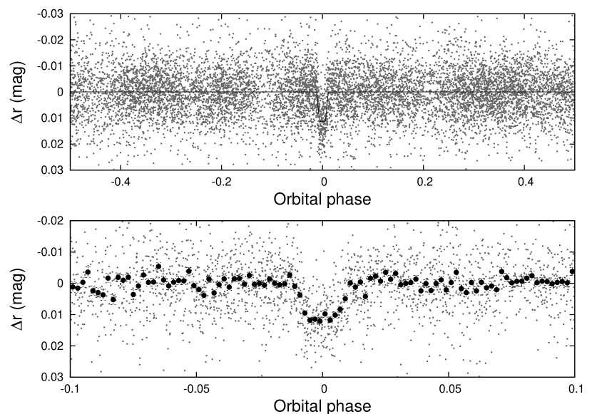
Figure 1.— Top panel: Unbinned photometric data of HAT-P-27 consisting of 9 400 Sloan $r$-band 5.5 minute cadence measurements obtained with HATNet telescopes, folded with period $P=3.039586$ d. A simple transit curve fit to the data points is displayed with a solid line. See Section 3.3 for details. Bottom panel: A close-up view of the transit. Small gray dots are the same folded data as above; large black dots show the light curve binned in phase using a bin size of 0.002.

Calibration, astrometry, aperture photometry, External Parameter Decorrelation (EPD), the Trend Filtering Algorithm (TFA) and the Box-fitting Least Squares method were applied to the data as described in Bakos et al. (2010a). We detected a transit signature in the light curve of HAT-P-27, with a signal depth of $10.6$ mmag and period of $P=3.0396$ days. This presumed transit has relative first-to-last-contact duration $q=0.0232\pm 0.0006$, corresponding to total duration $0.0705\pm 0.0019$ days ($1.693\pm 0.046$ hours). The folded light curve is presented in Figure 1.

2.2. Reconnaissance Spectroscopy

Reconnaissance spectra (Latham et al., 2009a) of HAT-P-27 were taken using three facilities: the Tillinghast Reflector Echelle Spectrograph (TRES; Fűrész, 2008) on the 1.5 m Tillinghast Reflector at FLWO, the echelle spectrograph on the 2.5 m du Pont telescope at Las Campanas Observatory (LCO) in Chile, and the echelle spectrograph on the Australian National University (ANU) 2.3 m telescope at Siding Spring Observatory (SSO) in Australia. We gathered two spectra of HAT-P-27 with TRES in 2009 July and 2010 February, two spectra with the du Pont telescope in 2009 July, and fourteen spectra with the ANU 2.3 m telescope in 2009 July. The exact dates and the results of these observations are summarized in Table 1.

Table 1 Summary of reconnaissance spectroscopy observations of HAT-P-27

Instrument	Date	Number of	$T_{\rm eff\star}$	$\log{g_{\star}}$	$v\sin{i}$	$\gamma_{\rm RV}$
		Spectra	(K)	(cgs)	($\rm km\,s^{-1}$)	($\rm km\,s^{-1}$)
TRES	2009 Jul 05	1	$5250$	$4.5$	$2$	$-15.75$
du Pont	2009 Jul 10	1	$5250$	$4.0$	$0$	$-16.03$
du Pont	2009 Jul 11	1	$5000$	$3.5$	$0$	$-18.03$
ANU 2.3 m	2009 Jul 16	5	$\cdots$	$\cdots$	$\cdots$	$-20.58$
ANU 2.3 m	2009 Jul 17	6	$\cdots$	$\cdots$	$\cdots$	$-21.32$
ANU 2.3 m	2009 Jul 18	3	$\cdots$	$\cdots$	$\cdots$	$-20.61$
TRES	2010 Feb 13	1	$5250$	$5.0$	$1$	$-15.78$

Following Quinn et al. (2010) and Buchhave et al. (2010), we calculated the mean radial velocity, effective temperature, surface gravity, and projected rotational velocity of the host star, based on spectra taken by TRES. The inferred radial velocity RMS residual of $0.05$ $\rm km\,s^{-1}$ is consistent with no detectable RV variation within the precision of the measurements. We established the following atmospheric parameters for HAT-P-27: effective temperature $T_{\rm eff\star}=5250\pm 100$ K, surface gravity $\log{g_{\star}}=4.75\pm 0.25$ (cgs), and projected rotational velocity $v\sin{i}=1.5\pm 1.0$ $\rm km\,s^{-1}$, indicating a G8 dwarf. The mean heliocentric RV of HAT-P-27 after subtracting the gravitational redshift of the Sun is $\gamma_{\rm RV}=-15.765\pm 0.51$ $\rm km\,s^{-1}$.

Because this is the first time we used the du Pont 2.5 m and ANU 2.3 m telescopes for reconnaissance spectroscopy of HATNet targets, we briefly describe the instruments and our data reduction procedure.

The spectrograph on the du Pont telescope was used with a $4\arcsec$ long and $1.5\arcsec$ wide slit. The obtained spectra have wavelength coverage $\approx$ 3700–7000 Å at a resolution of $\lambda/\Delta\lambda\approx 26\,000$. During the first observation the seeing ranged between 2–3″ and we used an exposure time of 1200 s, which provided $\sim 3000$ electrons per resolution element at the wavelength of 5187 Å. The seeing during the second observation was $\approx 1.8\arcsec$ and we used an exposure time of 150 s to obtain a lower S/N spectrum sufficient to detect a velocity variation of several $\rm km\,s^{-1}$. We obtained a ThAr lamp spectrum before and after each observation to use in determining the wavelength solution. We used the CCDPROC package of IRAF to perform overscan correction and flat-fielding of the images, and the ECHELLE package to extract the spectra and to determine and apply the dispersion corrections.

The extracted du Pont spectra were then cross-correlated against a library of synthetic stellar spectra to estimate the effective temperature, surface gravity, projected rotational velocity, and radial velocity of the star. We followed a procedure similar to that described by Torres et al. (2002), using the same synthetic templates, but broadened to the resolution of the du Pont echelle. These templates, which were generated for the CfA Digital Speedometer (Latham, 1992), only cover a wavelength range of 5150–5360 Å, so we restricted our analysis to a single order of the spectrum covering a similar range.

Spectra were also taken using the echelle spectrograph on the ANU 2.3 m telescope. The echelle was used in a standard configuration with a $1.8\arcsec$ wide slit and $300\;\mathrm{mm}^{-1}$ cross-disperser setting of $5^{\circ}50^{\prime}$, which delivered 27 full orders between 3900–6720 Å with a nominal spectral resolution of $\lambda/\Delta\lambda\approx 23\,000$. The CCD is a 2K$\times$2K format with $13.5\;\mu\mathrm{m}\times 13.5\;\mu\mathrm{m}$ pixels. The gain was two electrons per ADU resulting in a read noise of approximately 2.3 ADU for each pixel. The spectra were binned by two along the spatial direction. A total of fourteen 1200 s exposures were taken. The seeing ranged from $2\arcsec$ to $3\arcsec$. The signal-to-noise on a single pixel was between 5 and 10 for each individual exposure. ThAr lamp calibration exposures were taken every hour for wavelength calibration. A high signal-to-noise exposure was also taken of the bright radial velocity standard star HD 223311.

Spectra were reduced using tasks in the IRAF packages CCDPROC and ECHELLE. The spectra were cross-correlated against the radial velocity standard star HD 223311 using the IRAF task FXCOR in the RV package. We used at least 20, typically 25 of the 27 orders for the cross-correlation, rejecting the bluest orders for many exposures where the signal-to-noise was too low. Each spectral order was treated separately and the mean of the velocities from the individual orders was calculated. Their standard deviations were less than $0.65\;\rm km\,s^{-1}$ for each exposure.

Each night, the exposures were taken within a two hour interval, much shorter than the orbital period of the presumed companion. For detecting large radial velocity variations to rule out the possibility of an eclipsing binary, we consider the mean radial velocities per night. The standard deviations between exposures were less than $0.75\;\rm km\,s^{-1}$ for each night. Stellar parameters could have been estimated only with large uncertainty based on data with such low signal-to-noise. Therefore these parameters are not calculated from the ANU 2.3 m observations.

The results of the observations taken with these three telescopes are listed in Table 1. Note that for each telescope, the radial velocity measurement uncertainty is much higher than the radial velocity variations of the Sun due to Solar System bodies. Therefore we only calculated heliocentric radial velocities of the target. For the more accurate measurements described in the next section, we will use barycentric radial velocities instead. This accuracy, however, is enough to rule out the case of an eclipsing binary star with great certainty. The largest RV variation within an instrument was only 2 $\rm km\,s^{-1}$, much less than the orbital speed in a typical binary system. Note that the zero-point shift between instruments is as large as $\sim 5$ $\rm km\,s^{-1}$, due to the different methods used for data reduction. Also, all eighteen spectra were single-lined and spectral lines were symmetric, providing no evidence for additional stars in the system up to the precision of the measurements.

2.3. High resolution, high S/N spectroscopy

We acquired high-resolution, high-S/N spectra of HAT-P-27 using the HIRES instrument (Vogt et al., 1994) on the Keck I telescope located on Mauna Kea, Hawaii, between 2009 December and 2010 June. The spectrometer was configured with the $0.86\arcsec$ wide slit, yielding a resolving power of $\lambda/\Delta\lambda\approx 55\,000$ over the wavelength range of $\approx$ 3800–8000 Å.

Nine exposures were taken using an $\mathrm{I}_{2}$ gas cell (see Marcy & Butler, 1992), and a single template exposure was obtained without the absorption cell. We followed Butler et al. (1996) to establish RVs in the Solar System barycentric frame. We also calculated the $S$ index for each spectrum (following Isaacson & Fischer, 2010). The resulting values and their uncertainties are listed in Table 2. They are plotted period-folded in Figure 2, together with the fit established in Section 3.

Figure 2.— Top panel: Keck/HIRES RV measurements for HAT-P-27 shown as a function of orbital phase, along with our best-fit model (see Table 5). Zero phase corresponds to the time of mid-transit. The center-of-mass velocity has been subtracted. Second panel: Velocity $O\!-\!C$ residuals from the best fit. The error bars include a component from astrophysical/instrumental jitter ($6.3$ $\rm m\,s^{-1}$) added in quadrature to the formal errors (see Section 3.3). Third panel: Bisector spans (BS), with the mean value subtracted, and corrected for sky contamination. The measurement from the template spectrum is included (see Section 3.1). Bottom panel: Chromospheric activity index $S$. Again, the measurement from the template spectrum is included. Note: Panels have different vertical scales. The data point replotted in the second period is represented by an open symbol.

The effective temperature established later in Section 3.2 compared to Figure 4 of Valenti & Fischer (2005) implies $B-V=0.800$ for the star. This can in turn be used in the formula given in Noyes et al. (1984) together with the median $S_{\mathrm{HK}}$ of 0.231 to conclude $\log R^{\prime}_{\mathrm{HK}}=-4.785$. This activity value is consistent with the RV jitter value $6.3$ $\rm m\,s^{-1}$ established in Section 3.3, according to the observations given by Wright (2005). Based on Figure 9 in Isaacson & Fischer (2010), this value qualifies HAT-P-27 as chromospherically active relative to California Planet Search targets of the same spectral class. The activity index does not correlate significantly with orbital phase.

Table 2 Relative radial velocities, bisector spans, and activity index measurements of HAT-P-27

BJD (UTC)	RV	$\sigma_{\rm RV}$	BS	$\sigma_{\rm BS}$	$S$	Phase
($2\,400\,000+$)	($\rm m\,s^{-1}$)	($\rm m\,s^{-1}$)	($\rm m\,s^{-1}$)	($\rm m\,s^{-1}$)
$55192.13748$	$\cdots$	$\cdots$	$-4.96$	$3.92$	$0.211$	$0.013$
$55193.14273$	$-87.86$	$1.73$	$-2.89$	$5.30$	$0.212$	$0.344$
$55194.14692$	$73.31$	$1.51$	$-4.20$	$2.47$	$0.204$	$0.674$
$55252.00750$	$86.53$	$1.75$	$4.37$	$2.03$	$0.227$	$0.710$
$55257.15592$	$-51.27$	$1.84$	$1.11$	$3.44$	$0.244$	$0.404$
$55261.02101$	$84.94$	$2.02$	$-0.91$	$3.63$	$0.247$	$0.675$
$55290.06295$	$-84.71$	$1.89$	$3.14$	$3.57$	$0.245$	$0.230$
$55312.92780$	$98.63$	$2.08$	$-6.69$	$7.87$	$0.252$	$0.752$
$55374.90154$	$-74.42$	$1.85$	$-10.88$	$19.39$	$0.230$	$0.141$
$55375.82176$	$-29.80$	$2.10$	$-3.76$	$7.04$	$0.233$	$0.444$

Note. — For the iodine-free template exposures there is no RV measurement, but the BS and $S$ index can still be determined.

2.4. Photometric follow-up observations

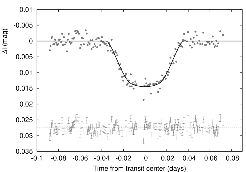
Figure 3.— Unbinned Sloan $i$-band transit light curve, acquired with KeplerCam on the FLWO 1.2 m telescope on 2010 March 2. The light curve has been EPD and TFA-processed. Our best fit from the global modeling is shown by the solid line. See Section 3.3 for details. Residuals from the fit are displayed at the bottom. The error bars represent the photon and background shot noise, plus the readout noise.

A high-precision photometric follow-up of a complete transit was carried out, permitting refined estimates of the light curve parameters and thus orbital and planetary properties: The transit of HAT-P-27 was observed on the night of 2010 March 2 with the KeplerCam CCD camera on the FLWO 1.2 m telescope. We acquired 168 science frames in Sloan $i$-band with 60 second exposure time, 73 second cadence.

Following the procedure described by Bakos et al. (2010a), these images were first calibrated, then astrometry and aperture photometry was performed to arrive at light curves, which were finally cleaned of trends using EPD and TFA, carried out simultaneously with the global modeling described in Section 3.3. The result is shown in Figure 3, along with the best-fit transit light curve; the individual measurements are reported in Table 3.

Table 3High-precision differential photometry of HAT-P-27

BJD (UTC)	Mag	$\sigma_{\rm Mag}$	Mag(orig)	Filter
($2\,400\,000+$)
$55258.88089$	$0.00295$	$0.00109$	$10.86800$	$i$
$55258.88157$	$0.00160$	$0.00109$	$10.86810$	$i$
$55258.88242$	$-0.00094$	$0.00095$	$10.86430$	$i$
$55258.88327$	$-0.00140$	$0.00094$	$10.86320$	$i$
$55258.88412$	$0.00104$	$0.00095$	$10.86640$	$i$
$55258.88499$	$0.00093$	$0.00094$	$10.86500$	$i$
$55258.88584$	$-0.00041$	$0.00095$	$10.86470$	$i$
$55258.88689$	$0.00056$	$0.00095$	$10.86350$	$i$
$55258.88773$	$0.00123$	$0.00094$	$10.86580$	$i$
$55258.88859$	$0.00098$	$0.00094$	$10.86540$	$i$

Note. — This table is available in a machine-readable form in the online journal. A portion is shown here for guidance regarding its form and content.

3. Analysis

3.1. Excluding blend scenarios

To further exclude possible blends, we perform bisector analysis the same way as in §5 of Bakos et al. (2007). A significant scatter is found, strongly correlated to the presence of moonlight, which we account for using the method described by Hartman et al. (2011). The bisector spans, corrected for the effect of the moonlight, are shown in the third panel of Figure 2. They do not exhibit significant correlation with the RV values, and the RMS scatter of the bisector spans (4.6 $\rm m\,s^{-1}$) is significantly smaller than the RV amplitude. These findings rule out a blend scenario with high certainty, implying that the measured photometric and spectroscopic features are due to a planet orbiting HAT-P-27.

3.2. Properties of the parent star

We first determine spectroscopic parameters of HAT-P-27, which will allow us to calculate stellar mass and radius. The Spectroscopy Made Easy analysis package (SME; Valenti & Piskunov, 1996) is used to establish the effective temperature, metallicity and stellar surface gravity based on the Keck/HIRES template spectrum of HAT-P-27, using atomic line data from the database of Valenti & Fischer (2005). After an initial estimate for these parameters, we perform a Monte Carlo calculation, relying also on the normalized semi-major axis $a/R_{\star}$ inferred from transit light curves, for the reasons described by Bakos et al. (2010b). The final values adopted after two iterations are $T_{\rm eff\star}=5300\pm 90$ K, $\rm[Fe/H]=+0.29\pm 0.10$, and $v\sin{i}=0.4\pm 0.4$ $\rm km\,s^{-1}$, also listed in Table 4.

Based on the final spectroscopic parameters the model isochrones yield a stellar mass $M_{\star}$ = $0.945\pm 0.035$ $M_{\sun}$ and radius $R_{\star}$ = $0.898_{-0.039}^{+0.054}$ $R_{\sun}$ for HAT-P-27, along with other properties listed at the bottom of Table 4. These values classify the star as a G8 dwarf, and suggest an age of $4.4_{-2.6}^{+3.8}$ Gyr. The model isochrones of Yi et al. (2001) for a metallicity of $+0.29$ are plotted in Figure 4, along with the best estimate of $a/R_{\star}$ and $T_{\rm eff\star}$ of HAT-P-27, and their $1\sigma$ and $2\sigma$ confidence ellipsoids. For comparison, the initial SME result, corresponding to a somewhat younger state, is also indicated.

Figure 4.— Model isochrones from Yi et al. (2001) for the measured metallicity of HAT-P-27, $\rm[Fe/H]$= $+0.29$, and ages running from 1 Gyr to 14 Gyr in 1 Gyr increments, left to right. The adopted values of $T_{\rm eff\star}$ and $a/R_{\star}$ are shown as the solid dot, surrounded by $1\sigma$ and $2\sigma$ confidence ellipsoids. The initial values of $T_{\rm eff\star}$ and $a/R_{\star}$ from the first SME and light curve analyses are represented with a triangle.

The intrinsic absolute magnitude predictions of this model (given in the ESO photometric system) can be compared to observations to calculate the distance of HAT-P-27. For this we use the near-infrared brightness measurements from the 2MASS Catalogue (Skrutskie et al., 2006): $J_{\rm 2MASS}=10.626\pm 0.026$, $H_{\rm 2MASS}=10.249\pm 0.023$ and $K_{\rm 2MASS}=10.109\pm 0.021$. These values are converted to ESO (Carpenter, 2001), then compared to the absolute magnitude estimates to calculate the distance. We account for interstellar dust extinction in the line of sight using $E(B\!-\!V)=0.036\pm 0.010$ from the dust map by Schlegel et al. (1998) with a conservative uncertainty estimate. This has to be multiplied by a factor depending on the distance of the star and its Galactic latitude (see Bonifacio et al., 2000). Assuming diffuse interstellar medium and no dense clouds along the line of sight, we use the value $R_{V}=3.1$, along with the coefficients given in Table 3 in Cardelli et al. (1989). These let us calculate extinction parameters for each band based on the reddening. Finally, comparing extinctions, absolute magnitude predictions and 2MASS apparent magnitudes for $J$, $H$ and $K$ bands, we arrive at separate distance estimates. These are in good agreement, yielding an average distance of $204\pm 14$ pc. The uncertainty does not account for possible systematics of the stellar evolution model. Note that this value is only 1 pc less than the more simple estimate ignoring extinction. The model predicts an unreddened color index of $(J-K)_{\mathrm{model}}=0.50\pm 0.04$. Reddening would change it to an estimated observed value of $(J-K)_{\mathrm{red}}=0.514\pm 0.04$ using the above parameters. This matches the actual observed color index $(J-K)_{\mathrm{ESO}}=0.550\pm 0.037$ within $1\sigma$.

Table 4 Stellar parameters for HAT-P-27

Parameter	Value	Source
Spectroscopic properties
$T_{\rm eff\star}$ (K)	$5300\pm 90$	SME
$\rm[Fe/H]$	$+0.29\pm 0.10$	SME
$v\sin{i}$ ($\rm km\,s^{-1}$)	$0.4\pm 0.4$	SME
$v_{\rm mac}$ ($\rm km\,s^{-1}$)	$3.29$	SME
$v_{\rm mic}$ ($\rm km\,s^{-1}$)	$0.85$	SME
$\gamma_{\rm RV}$ ($\rm km\,s^{-1}$)	$-15.765\pm 0.51$	TRES
Photometric properties
$V$ (mag)	12.214	TASS
$V\!-\!I_{C}$ (mag)	$0.527\pm 0.12$	TASS
$J$ (mag)	$10.626\pm 0.026$	2MASS
$H$ (mag)	$10.249\pm 0.023$	2MASS
$K_{s}$ (mag)	$10.109\pm 0.021$	2MASS
Derived properties
$M_{\star}$ ($M_{\sun}$)	$0.945\pm 0.035$	YY+$a/R_{\star}$+SME
$R_{\star}$ ($R_{\sun}$)	$0.898_{-0.039}^{+0.054}$	YY+$a/R_{\star}$+SME
$\log{g_{\star}}$ (cgs)	$4.51\pm 0.04$	YY+$a/R_{\star}$+SME
$L_{\star}$ ($L_{\sun}$)	$0.57_{-0.07}^{+0.09}$	YY+$a/R_{\star}$+SME
$M_{V}$ (mag)	$5.55\pm 0.17$	YY+$a/R_{\star}$+SME
$M_{K}$ (mag, ESO)	$3.62\pm 0.12$	YY+$a/R_{\star}$+SME
Age (Gyr)	$4.4_{-2.6}^{+3.8}$	YY+$a/R_{\star}$+SME
Distance (pc)	$204\pm 14$	YY+$a/R_{\star}$+SME

3.3. Global modeling of the data

We fit the combined model described by Bakos et al. (2010a) to the HATNet photometry, follow-up photometry, and radial velocity measurements simultaneously. The eight main parameters describing the model are the time of the first observed transit center, the time of the follow-up transit center, the normalized planetary radius $p\equiv R_{\mathrm{p}}/R_{\star}$, the square of the impact parameter $b^{2}$, the reciprocal of the half duration of the transit $\zeta/R_{\star}$, the RV semi-amplitude $K$, and the Lagrangian elements $k\equiv e\cos\omega$ and $h\equiv e\sin\omega$ (where $\omega$ is the longitude of periastron).

Instrumental parameters of the model include the HATNet out-of-transit magnitude and the relative zero-point of the Keck RVs. The joint fit provides the full a posteriori probability distributions of all variables (including $\log{g_{\star}}$), which are used to update the limb-darkening coefficients for another iteration of the joint fit. This leads to estimated distributions for the stellar, light curve, and RV parameters, which are combined to calculate values for planetary parameters. These final values are summarized in Table 5.

The orbital eccentricity is consistent with zero (using the method of Lucy & Sweeney, 1971 we find that there is a 25% conditional probability of detecting an eccentricity of at least 0.078 given a circular orbit and an uncertainty of 0.047). Nevertheless, we stress that throughout the global modeling, the orbit was allowed to be eccentric, and all system parameters and their respective errors inherently contain the uncertainty arising from the floating $k$ and $h$ values.

Table 5Orbital and planetary parameters

Parameter	Value
Light curve parameters
$P$ (days)	$3.039586\pm 0.000012$
$T_{c}$ (BJD, UTC)	$2455186.01879\pm 0.00054$
$T_{14}$ (days)	$0.0705\pm 0.0019$
$T_{12}=T_{34}$ (days)	$0.0214\pm 0.0053$
$a/R_{\star}$	$9.65_{-0.54}^{+0.40}$
$\zeta/R_{\star}$	$38.20\pm 0.80$
$R_{\mathrm{p}}/R_{\star}$	$0.1186\pm 0.0031$
$b^{2}$	$0.690_{-0.032}^{+0.029}$
$b\equiv a\cos i/R_{\star}$	$0.831_{-0.020}^{+0.017}$
$i$ (degree)	$84.7_{-0.7}^{+0.4}$
Limb-darkening coefficients
$a_{i}$ (linear term)	$0.3627$
$b_{i}$ (quadratic term)	$0.2816$
RV parameters
$K$ ($\rm m\,s^{-1}$)	$96.1\pm 4.5$
$k_{\rm RV}$	$0.036\pm 0.031$
$h_{\rm RV}$	$0.066\pm 0.048$
$e$	$0.078\pm 0.047$
$\omega$ (degree)	$63\pm 64$
RV jitter ($\rm m\,s^{-1}$)	$6.3$
Secondary eclipse parameters
$T_{s}$ (BJD)	$2455187.608\pm 0.060$
$T_{s,14}$	$0.0739\pm 0.0061$
$T_{s,12}$	$0.0368\pm 0.0066$
Planetary parameters
$M_{\mathrm{p}}$ ($M_{\rm J}$)	$0.660\pm 0.033$
$R_{\mathrm{p}}$ ($R_{\rm J}$)	$1.038_{-0.058}^{+0.077}$
$C(M_{\mathrm{p}},R_{\mathrm{p}})$	$0.310$
$\rho_{\mathrm{p}}$ ($\rm g\,cm^{-3}$)	$0.73\pm 0.13$
$\log g_{p}$ (cgs)	$3.18\pm 0.05$
$a$ (AU)	$0.0403\pm 0.0005$
$T_{\rm eq}$ (K)	$1207\pm 41$
$\Theta$	$0.054\pm 0.004$
$F_{per}$ ($10^{8}$ $\rm erg\,s^{-1}\,cm^{-2}$)	$5.61_{-0.87}^{+1.64}$
$F_{ap}$ ($10^{8}$ $\rm erg\,s^{-1}\,cm^{-2}$)	$4.09\pm 0.48$
$\langle F\rangle$ ($10^{8}$ $\rm erg\,s^{-1}\,cm^{-2}$)	$4.79_{-0.56}^{+0.78}$

4. Discussion

4.1. Properties of HAT-P-27b

Figure 5 presents the currently known transiting exoplanets and Solar System gas planets on a mass—radius diagram, with HAT-P-27b highlighted. Also shown are the planetary isochrones of Fortney et al. (2007) interpolated to the insolation of HAT-P-27 at the orbit of HAT-P-27b. Taking into consideration the age established in Section 3.2, the planetary parameters are consistent with a hot Jupiter with a 10 $M_{\earth}$ core in a 4 Gyr old system.

HAT-P-27b can be seen to lie inside the large accumulation of planets with similar masses and radii. To further compare it to other Hot Jupiters, in Figure 6 we present histograms of mass, radius and period for the 112 transiting exoplanets confirmed to date.

When comparing these parameters, we note that there is only one transiting exoplanet known that is more massive and has a smaller radius and a smaller period than HAT-P-27b: this is HAT-P-20b with 7.246 $M_{\rm J}$, 0.867 $R_{\rm J}$ on a 2.875 d orbit (Bakos et al., 2010b). This means that HAT-P-27b is less inflated than other planets of similar mass and orbital period, possibly due to a larger than average core.

Regarding eccentricity, there are 31 transiting exoplanets known under 8 $M_{\rm J}$ with an orbital period within 0.5 d of that of HAT-P-27b, out of which 8 – more than a quarter of them – are thought to be eccentric. This hints that there is a possibility for the orbit of HAT-P-27b to be eccentric as well, justifying our choice not to fix eccentricity to zero in Section 3. Future observations of radial velocity or occultation timing would be required to determine whether the orbit is indeed eccentric.

The impact parameter of HAT-P-27b is unusually large. As Ribas et al. (2008) pointed out, such a near grazing transit has the advantage of its depth and duration being more sensitive to the presense of further planetary companions on inclined orbits. This makes HAT-P-27 a promising target for transit timing variation and transit duration variation studies.

Knutson et al. (2010) found a strong negative correlation between chromospheric activity of the host star and temperature inversion in the planetary atmosphere. However, since early type stars dominate magnitude limited surveys, cool, that is, active planetary hosts are rare. The bottom right panel of Figure 6 shows that HAT-P-27 is relatively active compared to known planetary hosts for which $\log R^{\prime}_{\mathrm{HK}}$ has been reported, making it an exciting target for Spitzer Space Telescope to test this correlation.

4.2. Correlation of planetary parameters with host star metallicity

The relation between host star metallicity (denoted as $\rm[Fe/H]_{\star}$ for clarity, not to be confused with the assumed metal content of the planet) and planetary composition was studied by Guillot et al. (2006). A positive correlation, with Pearson correlation coefficient $r=0.78$, was found between the inferred mass of the planetary core and stellar metallicity for the seven transiting exoplanets known at that time with positive inferred core mass. The idea is that planets have formed from the same cloud as their host stars, and therefore their metal content should correlate. However, it is not clear how stellar metallicity is connected to planetary metallicity, especially because a larger rocky core is likely to accrete more gas during the planet’s formation.

Burrows et al. (2007) also investigated this relation, based on 12 transiting exoplanets known at the time. They used an atmospheric opacity dependent core mass model to explain radius anomalies. They also found a strong correlation between host star metallicity and inferred core mass, but the correlation coefficient was not reported.

Enoch et al. (2010) found that there is a strong negative correlation with $r=-0.53$ between $\rm[Fe/H]_{\star}$ and $R_{\mathrm{p}}$ for the 18 known transiting exoplanets below 0.6 $M_{\rm J}$, whereas this correlation is negligible for more massive planets. This can be explained by noticing that the theoretical planet models of Fortney et al. (2007), Bodenheimer et al. (2003), and Baraffe et al. (2008) all suggest that the radius of a planet is more sensitive to its composition for low mass planets than it is for more massive ones.

Table 6 Parameters of 30 transiting exoplanets between 0.3 $M_{\rm J}$ and 0.8 $M_{\rm J}$ in increasing order of mass

name	$M_{\mathrm{p}}(M_{\rm J})$	$R_{\mathrm{p}}(R_{\rm J})$	$T_{\rm eff}(\mathrm{K})$	$\rm[Fe/H]_{\star}$	reference
WASP-21b	$0.3\pm 0.01$	$1.07\pm 0.05$	$1262\pm 31$	$-0.4\pm 0.1$	Bouchy et al. (2010)
HD 149026b	$0.368^{+0.013}_{-0.014}$	$0.813^{+0.027}_{-0.025}$	$1792^{+44}_{-32}$	$+0.36\pm 0.05$	Ammler-von Eiff et al. (2009),
					Carter et al. (2009)
Kepler-7b	$0.416^{+0.036}_{-0.035}$	$1.439^{+0.058}_{-0.056}$	$1565^{+31}_{-30}$	$+0.11\pm 0.03$	Latham et al. (2009b),
					Kipping & Bakos (2010)
WASP-13b	$0.46^{+0.056}_{-0.05}$	$1.21^{+0.14}_{-0.12}$	$1417^{+62}_{-58}$	$+0.0\pm 0.2$	Skillen et al. (2009)
Kepler-8b	$0.46\pm 0.14$	$1.31^{+0.076}_{-0.08}$	$1628^{+52}_{-53}$	$-0.055\pm 0.03$	Jenkins et al. (2010),
					Kipping & Bakos (2010)
CoRoT-5b	$0.467^{+0.047}_{-0.024}$	$1.388^{+0.046}_{-0.047}$	$1438\pm 39$	$-0.25\pm 0.06$	Rauer et al. (2009)
WASP-31b	$0.478\pm 0.03$	$1.54\pm 0.06$	$1568\pm 33$	$-0.19\pm 0.09$	Anderson et al. (2010)
WASP-11/HAT-P-10b	$0.487\pm 0.018$	$1.005^{+0.032}_{-0.027}$	$1020\pm 17$	$+0.13\pm 0.08$	Bakos et al. (2009)
WASP-17b	$0.49^{+0.059}_{-0.056}$	$1.74^{+0.26}_{-0.23}$	$1662^{+113}_{-110}$	$-0.25\pm 0.09$	Anderson et al. (2010)
WASP-6b	$0.503^{+0.019}_{-0.038}$	$1.224^{+0.051}_{-0.052}$	$1194^{+58}_{-57}$	$-0.20\pm 0.09$	Gillon et al. (2009)
HAT-P-1b	$0.524\pm 0.031$	$1.225\pm 0.059$	$1306\pm 30$	$+0.21\pm 0.03$	Torres et al. (2008),
					Ammler-von Eiff et al. (2009)
HAT-P-17b	$0.53\pm 0.019$	$1293\pm 0.03$	$787\pm 15$	$+0.0\pm 0.08$	Howard et al. (2010)
WASP-15b	$0.542\pm 0.05$	$1.428^{+0.077}_{-0.077}$	$1652\pm 28$	$-0.17\pm 0.11$	West et al. (2009)
OGLE-TR-111b	$0.55\pm 0.1$	$1.019^{+0.026}_{-0.026}$	$1025^{+26}_{-25}$	$+0.19\pm 0.07$	Santos et al. (2006),
					Torres et al. (2008),
					Adams et al. (2010)
HAT-P-4b	$0.556\pm 0.068$	$1.367^{+0.052}_{-0.044}$	$1686^{+30}_{-26}$	$+0.24\pm 0.08$	Kovács et al. (2007),
					Torres et al. (2008),
					Winn et al. (2010)
WASP-22b	$0.56\pm 0.02$	$1.12\pm 0.04$	$1430\pm 30$	$-0.05\pm 0.08$	Maxted et al. (2010)
XO-2b	$0.566^{+0.055}_{-0.055}$	$0.983^{+0.029}_{-0.028}$	$1319^{+24}_{-23}$	$0.44\pm 0.04$	Torres et al. (2008),
					Ammler-von Eiff et al. (2009)
HAT-P-25b	$0.567\pm 0.022$	$1.19^{+0.081}_{-0.056}$	$1202\pm 36$	$+0.31\pm 0.08$	Quinn et al. (2010)
WASP-25b	$0.58\pm 0.04$	$1.22^{+0.06}_{-0.05}$	$1212\pm 35$	$-0.07\pm 0.1$	Enoch et al. (2010)
WASP-34b	$0.59\pm 0.01$	$1.22^{+0.11}_{-0.08}$	$1250\pm 30$	$-0.02\pm 0.1$	Smalley et al. (2010)
HAT-P-3b	$0.596^{+0.024}_{-0.026}$	$0.899^{+0.043}_{-0.049}$	$1127^{+49}_{-39}$	$+0.27\pm 0.04$	Torres et al. (2007),
					Torres et al. (2008)
HAT-P-28b	$0.636\pm 0.037$	$1.189^{+0.102}_{-0.075}$	$1371\pm 50$	$+0.12\pm 0.08$	Buchhave et al. (2011)
HAT-P-27b	$0.660\pm 0.033$	$1.038^{+0.077}_{-0.058}$	$1207\pm 41$	$+0.29\pm 0.1$	this paper
HAT-P-24b	$0.685\pm 0.033$	$1.242\pm 0.067$	$1637\pm 42$	$-0.16\pm 0.08$	Kipping et al. (2010)
HD 209458b	$0.685^{+0.015}_{-0.014}$	$1.359^{+0.016}_{-0.019}$	$1449\pm 12$	$+0.01\pm 0.03$	Laughlin et al. (2005),
					Torres et al. (2008)
Kepler-6b	$0.62^{+0.025}_{-0.028}$	$1.164^{+0.025}_{-0.017}$	$1459^{+25}_{-24}$	$+0.34\pm 0.04$	Dunham et al. (2010),
					Kipping & Bakos (2010)
OGLE-TR-10b	$0.62\pm 0.14$	$1.25^{+0.14}_{-0.12}$	$1481^{+71}_{-55}$	$+0.15\pm 0.15$	Torres et al. (2008)
CoRoT-4b	$0.72\pm 0.08$	$1.19^{+0.06}_{-0.05}$	$1074\pm 19$	$+0.05\pm 0.07$	Moutou et al. (2008)
TrES-1b	$0.752^{+0.047}_{-0.046}$	$1.067^{+0.022}_{-0.021}$	$1140^{+13}_{-12}$	$+0.02\pm 0.05$	Torres et al. (2008)
HAT-P-9b	$0.780\pm 0.090$	$1.40\pm 0.06$	$1530\pm 40$	$+0.12\pm 0.2$	Shporer et al. (2009)

In this subsection, we examine further the correlation between host star metallicity and planetary mass or planetary radius. We use a substantially expanded sample of 30 known transiting exoplanets with masses between 0.3 $M_{\rm J}$ and 0.8 $M_{\rm J}$, see Table 6. The upper limit is selected to exclude more massive planets whose radius is expected to depend less on the composition, see above. We explain the role of the lower limit and the effect of the two lowest mass planets in Table 6 later.

The null hypothesis is that the host star metallicity and the selected planetar parameter are independent. The alternative hypothesis is that they are related by some underlying phenomenon. A false positive, also known as an error of the first kind, is rejection of the null hypothesis in spite of it being true. We implement three independent statistical methods to estimate the false positive probability: $t$-test, bootstrap technique and $F$-test. We denote the probability estimates by $p_{1}$, $p_{2}$ and $p_{3}$, respectively. This is the statistical significance of the correlation: the lower this probability is, the more confidently the null hypothesis (i.e., no correlation) can be rejected.

For the $t$-test, we assume that the investigated parameters have normal distribution. For each set of data pairs, we calculate the $t$ value from the correlation coefficient $r$ and sample size $n$ using the formula

$$t=r\sqrt{\frac{n-2}{1-r^{2}}}\;.$$

The conditional distribution of this variable given the null hypothesis is Student’s $t$ distribution with $n-2$ degrees of freedom (Press et al., 1992, p. 640). Then the estimate $p_{1}$ for false positive probability is determined by looking up the two-tailed probability of this distribution yielding larger absolute value that the one measured. For comparison, we also performed the $t$-test for the samples and parameters studied by Guillot et al. (2006) and Enoch et al. (2010). The resulting values are listed in Table 7.

For the sample set of Table 6, we also implement the bootstrap resampling technique (Efron & Tibshirani, 2003). This has the advantage that no assumption about the a priori distribution of the data is necessary. To perform bootstrap resampling, consider the data $(x_{1},y_{1}),(x_{2},y_{2}),\ldots,(x_{n},y_{n})$, where $x_{i}$ is the host star metallicity, and $y_{i}$ is the corresponding planetary mass or radius. Again, we would like to calculate an estimate $p_{2}$ of the probability that a sample of similar distribution, but independent parameters for each pair, has a correlation coefficient that exceeds that of our measurements in absolute value. For this, we build 10 000 000 sample sets of $n$ pairs by drawing $x$ and $y$ values independently with replacements from the set of measured $x$ and $y$ values, respectively. The percentile rank of the absolute value of the correlation coefficient for the measured data among the random samples gives our estimates $p_{2}$, listed in Table 7.

Finally, we test these correlations with an additional method, the $F$-test (see e.g. Lupton, 1993, p. 100). This requires that the null hypothesis (no correlation) be nested in the tested hypothesis (linear correlation), which indeed is the case. Let RSS₁ denote the residual sum of squares for the best fit of the null hypothesis, that is, the variance of $y_{i}$ about its mean, and RSS₂ denote the residual sum of squares of the linear fit. The no correlation model has $l_{1}=1$ free parameters: the mean, whereas the linear fit has $l_{2}=2$. The conditional distribution of

$$F=\frac{\frac{\mathrm{RSS}_{1}-\mathrm{RSS}_{2}}{l_{2}-l_{1}}}{\frac{\mathrm{RSS}_{2}}{n-l_{2}}}$$

given the null hypothesis is the $F$-distribution with $(l_{2}-l_{1},n-l_{2})$ degrees of freedom. This enables us to calculate $p_{3}$, the third estimate for the false positive probability.

The estimates $p_{1}$, $p_{2}$, $p_{3}$ given by the three methods are listed in Table 7. For each correlation, they coincide up to the uncertainty of the methods. The values reflect the significant $\rm[Fe/H]_{\star}\textrm{---}M_{core}$ and $\rm[Fe/H]_{\star}\textrm{---}R_{\mathrm{p}}$ correlations found by Guillot et al. (2006) and Enoch et al. (2010).

As for the 30 planets listed in Table 6, it is important to note that the correlations depend strongly on the choice of the lower mass limit. The two least massive planets in the table are WASP-21b with a mass of $0.3\;M_{\rm J}$, very low host star metallicity of $-0.4$, and average radius of $1.07\;R_{\rm J}$; and the dense HD 149026b with a mass of $0.368\;M_{\rm J}$, high host star metallicity of $+0.36$, and low radius of $0.813\;R_{\rm J}$. Increasing the lower mass limit for our sample first excludes WASP-21b, which would much support the positive $\rm[Fe/H]_{\star}$—$M_{\mathrm{p}}$ correlation with its low mass and low host star metallicity. Further increasing the limit then excludes HD 149026b, which would much weaken it with its low mass and high host star metallicity. To have an unbiased result, outliers cannot be excluded without a justified reason, therefore we need to compare the false positive probabilities of the three nested samples. They scatter between 15% and 58%, neither supporting, nor rejecting a $\rm[Fe/H]_{\star}$—$M_{\mathrm{p}}$ correlation.

Similarily, both WASP-21b and HD 149026b have a strong effect on the negative $\rm[Fe/H]_{\star}$—$R_{\mathrm{p}}$ correlation, because of the extreme value of their host star metallicities. In this case, we see that the maximum of the false positive probabilities is $0.44\%$, therefore this correlation is statistically significant for all our choices of lower mass limits. This is at least a fivefold improvement over the sample investigated by Enoch et al. (2010), due to the larger sample size.

Table 7 Correlation between the host star metallicity and planetary parameters for known transiting exoplanets

Restriction			$n$	Planetary	$r$		$p_{1}$		$p_{2}$		$p_{3}$
on planets				parameter
$0<$	$M_{\mathrm{core}}$		7	$M_{\mathrm{core}}$	0.	78	3.	9%
	$M_{\mathrm{p}}$	$<0.6$ $M_{\rm J}$	18	$R_{\mathrm{p}}$	-0.	53	2.	4%
0.3 $M_{\rm J}\leqslant$	$M_{\mathrm{p}}$	$\leqslant 0.8$ $M_{\rm J}$	30	$M_{\mathrm{p}}$	0.	270	15.	0%	15.	0%	15.	0%
0.35 $M_{\rm J}\leqslant$	$M_{\mathrm{p}}$	$\leqslant 0.8$ $M_{\rm J}$	29	$M_{\mathrm{p}}$	0.	106	58.	4%	58.	2%	58.	4%
0.4 $M_{\rm J}\leqslant$	$M_{\mathrm{p}}$	$\leqslant 0.8$ $M_{\rm J}$	28	$M_{\mathrm{p}}$	0.	247	20.	4%	20.	4%	20.	4%
0.3 $M_{\rm J}\leqslant$	$M_{\mathrm{p}}$	$\leqslant 0.8$ $M_{\rm J}$	30	$R_{\mathrm{p}}$	-0.	505	0.	44%	0.	43%	0.	44%
0.35 $M_{\rm J}\leqslant$	$M_{\mathrm{p}}$	$\leqslant 0.8$ $M_{\rm J}$	29	$R_{\mathrm{p}}$	-0.	620	0.	03%	0.	03%	0.	034%
0.4 $M_{\rm J}\leqslant$	$M_{\mathrm{p}}$	$\leqslant 0.8$ $M_{\rm J}$	28	$R_{\mathrm{p}}$	-0.	575	0.	14%	0.	14%	0.	14%

4.3. Dependence on planetary equilibrium temperature

Other factors like insolation are likely to influence planetary radius as well, see e.g. Fortney et al. (2007), Kovács et al. (2010), Enoch et al. (2010), and Faedi et al. (2011). To further investigate this relation, we compare two models: for null hypothesis, we accept the linear planetary radius—host star metallicity relation of the previous section:

$$\tilde{}R_{\mathrm{p}}^{\mathrm{I}}=R_{0}^{\mathrm{I}}+\alpha^{\mathrm{I}}\cdot\rm[Fe/H]_{\star}.$$ (1)

The second model – alternative hypothesis – is similar to that of Enoch et al. (2010), accounting for the equilibrium temperature $T_{\mathrm{eq}}$ in addition to the host star metallicity:

$$\tilde{}R_{\mathrm{p}}^{\mathrm{II}}=R_{0}^{\mathrm{II}}+\alpha^{\mathrm{II}}\cdot\rm[Fe/H]_{\star}+\beta^{\mathrm{II}}\cdot T_{\mathrm{eq}}.$$ (2)

The equilibrium temperature of the planet is calculated from the time-averaged stellar flux on its orbit, assuming gray body spectrum for the planets, and neglecting tidal and other heating mechanisms. For simplicity, we now include all 30 planets of Table 6 in our models. With the best fit parameters, the two models are

$$\tilde{}R_{\mathrm{p}}^{\mathrm{I}} = 1.235\,R_{\rm J}{}-0.478\,R_{\rm J}{}\cdot\rm[Fe/H]_{\star},$$

$$\tilde{}R_{\mathrm{p}}^{\mathrm{II}} = 0.690\,R_{\rm J}{}-0.431\,R_{\rm J}{}\cdot\rm[Fe/H]_{\star}+0.398\,R_{\rm J}\cdot\frac{T_{\mathrm{eq}}}{1000\,\mathrm{K}}.$$

To quantify the statistical significance, we apply the $F$-test again. The resulting false positive probability is 0.18%. This means that once we accept the dependence of planetary radius on host star metallicity, then the probability of such a correlation with planetary equilibrium temperature if they were not physically related is only 0.18%. This strongly supports the three-parameter linear fit model. For reference, the residual sums of squares for the one, two and three-parameter fits of the $\rm[Fe/H]_{\star}$—$R_{\mathrm{p}}$ data are $1.13\;R_{\rm J}^{2}$, $0.84\;R_{\rm J}^{2}$ and $0.58\;R_{\rm J}^{2}$, respectively.

Figure 7 presents $R_{\mathrm{p}}-\beta^{\mathrm{II}}\cdot T_{\mathrm{eq}}$ versus metallicity for the 30 planets. Equation (2) predicts this quantity to be $R_{0}^{\mathrm{II}}+\alpha^{\mathrm{II}}\cdot\rm[Fe/H]_{\star}$, which is also plotted. HAT-P-27b apparently follows the model’s prediction. For reference, the correlation coefficient between the displayed transformed variables is now $r^{\mathrm{II}}=-0.536$, which has a larger absolute value than $r^{\mathrm{I}}=-0.505$ between $R_{\mathrm{p}}$ and metallicity, as expected.

This analysis supports the statement that planetary radius depends on equilibrium temperature in addition to host star metallicity, as found by Enoch et al. (2010) and Faedi et al. (2011). However, this correlation does not imply that insolation itself would inflate planets: the underlying phenomenon could be related to anything correlated to equilibrium temperature, or equivalently, orbital radius. For instance, Batygin & Stevenson (2010) suggest that it is Ohmic dissipation in the interior of the planet that inflates hot Jupiters. This theory is further supported by Laughlin et al. (2011).

Altogether, HAT-P-27b is an important addition to the growing sample of low-mass Jupiters. It orbits a metal rich star, and supports the suggested correlations between host star metallicity, planetary equilibrium temperature, and planetary radius. Also, HAT-P-27 is chromospherically active, providing an excellent case for refining the confidence level of the hypothesized correlation between stellar activity and planetary temperature inversion.

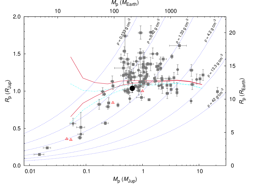
Figure 5.— Mass–radius diagram showing HAT-P-27b (solid black circle), other HATNet planets (solid gray circles), other known transiting exoplanets (solid gray squares), and Solar System gas giants (empty red triangles). Overlaid are Fortney et al. (2007) planetary isochrones interpolated to the solar equivalent semi-major axis of HAT-P-27b for ages of 1 Gyr (solid crimson lines) and 4 Gyr (dashed-dotted cyan lines) and core masses of 0 and 10 $M_{\earth}$ (upper and lower pairs of lines respectively). Isodensity curves are shown for 0.133, 0.42, 1.33 (Jupiter density), 4.2, 13.3, and 42 $\rm g\,cm^{-3}$(dashed lines).

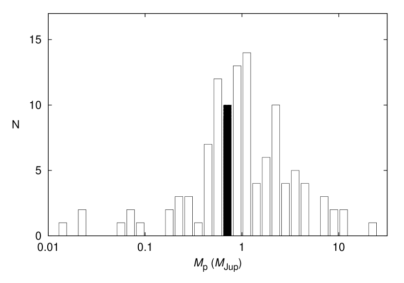
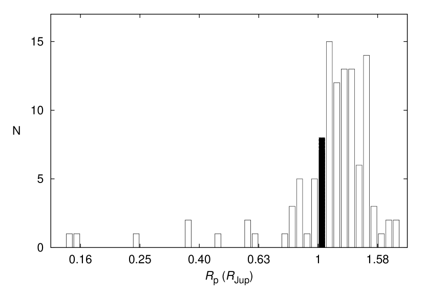
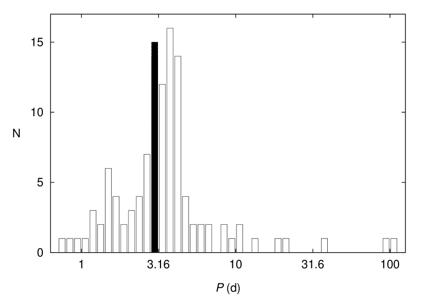
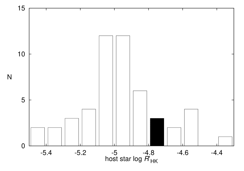
Figure 6.— Distribution of planetary and stellar parameters for transiting exoplanets known to date. Horizontal axes and bins are logarithmic except for $\log R^{\prime}_{\mathrm{HK}}$. Vertical axes show the number of planets in each bin, and the bin containing HAT-P-27b has solid filling. Top left panel: histogram of planetary mass in Jupiter masses, with logarithmic bin size 0.2. Top right panel: histogram of planetary radius in Jupiter radii, with logarithmic bin size 0.025. Bottom left panel: histogram of period in days, with logarithmic bin size 0.05. Bottom right panel: histogram of $\log R^{\prime}_{\mathrm{HK}}$, with bin size 0.1. This index has only been reported for 52 host stars.

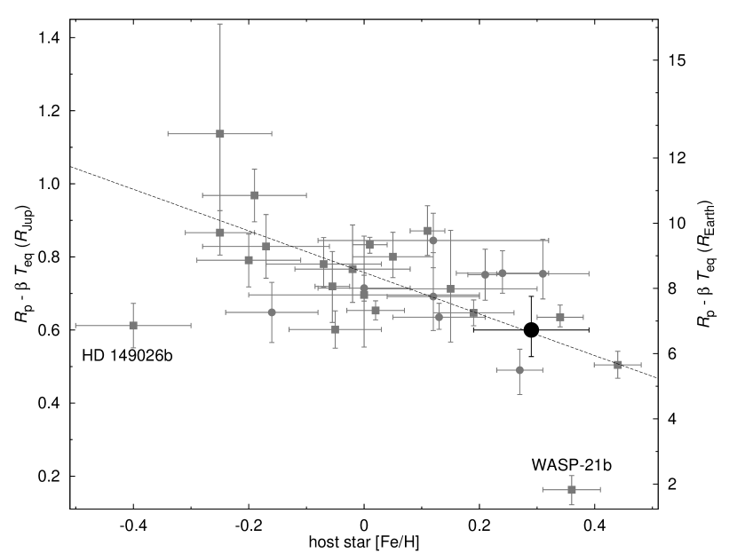
Figure 7.— Planetary radius corrected for linear equilibrium temperature dependence in Jupiter radii versus host star metallicity for the 30 known transiting exoplanets with masses between 0.3 $M_{\rm J}$ and 0.8 $M_{\rm J}$, including HAT-P-27b (solid black circle), other HATNet planets (solid gray circles), and other known transiting exoplanets (solid gray squares, WASP-21b and HD 149026b labeled); with best linear fit overlaid (dashed line).

References

- Adams et al. (2010) Adams, E. R., López-Morales, M., Elliot, J. L., Seager, S., & Osip, D. J. 2010, arXiv:1003.0457