Complex networks and glassy dynamics: walks in the energy landscape

Abstract

We present a simple mathematical framework for the description of the dynamics of glassy systems in terms of a random walk in a complex energy landscape pictured as a network of minima. We show how to use the tools developed for the study of dynamical processes on complex networks, in order to go beyond mean-field models that consider that all minima are connected to each other. We consider several possibilities for the transition rates between minima, and show that in all cases the existence of a glassy phase depends on a delicate interplay between the network’s topology and the relationship between energy and degree of a minimum. Interestingly, the network’s degree correlations and the details of the transition rates do not play any role in the existence (nor in the value) of the transition temperature, but have an impact only on more involved properties. For Glauber or Metropolis rates in particular, we find that the low-temperature phase can be further divided into two regions with different scaling properties of the average trapping time. Overall, our results rationalize and link the empirical findings about correlations between the energy of the minima and their degree, and should stimulate further investigations on this issue.

1 Introduction

In the last decade, studies about the structure and dynamics of complex networks have blossomed, thanks in particular to the versatility of the network representation, which has turned out to be adequate for systems as diverse as the Internet or social networks. A large body of knowledge about the empirical description of networked systems has thus been accumulated, together with a wealth of modeling techniques; a good level of understanding of how dynamical processes taking place on networks depend on their structure has been as well reached [1, 2, 3, 4, 5, 6]. Many network studies have been concerned with systems of interest in several scientific areas a priori remote from physics (social sciences, biology, computer science, epidemiology, …), and they have also reached more traditional fields of statistical physics, such as the study of glassy systems, as we now describe.

The many puzzles raised by the glass transition, and in particular the slow dynamics displayed by glassy systems at low temperatures, have been the subject of a large interest in the past decades [7, 8]. One of the approaches which has led to promising insights consists in the description of the dynamics of a glassy system inside its configuration space. The energy landscape of a glassy system is typically rugged, made of many local minima (metastable states), whose huge number makes it difficult to reach equilibrium. In this framework, the energy landscape is seen as a set of basins of attractions of local minima (“traps”), and the system evolves through a succession of harmonic vibrations inside traps and jumps between minima [9, 10]. This picture has stimulated the definition and study of various simplified models of dynamical evolution between traps, in order to reproduce the phenomenology of glassy dynamics [11, 12, 13, 14, 15, 16, 17]. On the other hand, several studies have focused on obtaining a better understanding of the structure of these local minima. A way to attain this goal is to perform numerical simulations of small systems, at a fixed temperature, and quenching them at regular time intervals in order to make them reach the nearest local minimum. Information is then gathered on the various local minima, and on the sizes of their basins of attraction. Various studies have investigated, among other issues, the detailed structure of the potential energy landscape, the substructure of minima, and the properties of energy barriers between minima [18, 19, 20]. Several works have also used the information on the energy landscape to study a master equation for the time evolution of the probability to be in each minimum. The considered systems range from clusters of Lennard-Jones atoms to proteins or heteropolymers [9, 10, 21, 22, 23].

An interesting property of the modeling of the energy landscape in terms of a set of traps linked by energy barriers, lies in the possibility to define and study its network representation within the context of network theory. In this representation, each local minimum is associated to a node, and a link is drawn between two nodes whenever it is possible for the system to jump between the basins of attraction of the corresponding minima. The links can then be defined as weighted and directed, as jumps between minima are not equiprobable, and may be easier in one direction than in the other. Networks of local minima of the energy landscape have thus been built and studied. These networks have been found to exhibit a small-world character [24]. The number of links of each node (its degree) turns out to be strongly heterogeneous, possibly with scale-free degree distributions, which have been linked to scale-free distributions of the areas of the basins of attraction [25, 26, 27]. Complex network analysis tools have also been used to investigate the structure of energy landscapes of various systems of interest, such as Lennard-Jones atoms, proteins, or spin glasses, among others [21, 22, 23, 27, 28, 29, 30, 31, 32, 33]. The energy of a minimum and its degree (i.e., the number of other minima which can be reached from this minimum) have been shown to be correlated, as well as the barriers to overcome to escape from a minimum. In particular, a logarithmic dependence of the energy of a minimum on its degree has been exhibited, as well as energy barriers increasing as a (small) power of the degree of a node [23, 25, 27]. No systematic study of these issues has however been performed, and most investigations have been limited to relatively small systems because of computational limitations.

Most importantly, the investigations cited above have focused on the topology of the network of minima, conceived as a tool to characterize the energy landscape. The structure of a network has however a deep impact on the properties of the dynamical processes which take place on it [6]. It seems thus adequate to put to use the tools and techniques developed for the analysis of dynamical processes on networks to achieve a better understanding of how the energy landscape structure, represented as a network, affects the system performing a random walk in it, and how the onset of glassy dynamics can be described in this way in a general framework. In a previous paper [34], we have made a first step to fill this gap by focusing on the trap model put forward in Ref. [11]. In this paper, we generalize our approach to more involved transition rates between energy minima. We show how the heterogeneous mean-field (HMF) theory [6, 35] can be used in this context to highlight the connection between the topological properties of the network of minima and the dynamical exploration of these minima. We show in particular that the relationship between energy and degree of the minima is a crucial ingredient for the existence of a transition and the subsequent glassy phenomenology. Our results shed light on the empirically found relationship between the energy of a local minimum and its degree, and we hope that they will stimulate more systematic investigations on this issue.

We have organized our paper as follows: In Section 2 we define our model of energy landscape dynamics as a random walk on a complex network. Different physical transition rates are proposed, and the corresponding numerical implementation is discussed. In Section 3 we present a theoretical analysis based on the heterogeneous mean-field approximation for dynamical processes on complex networks. This formalism is applied in Section 4, where general analytical approximate expression are presented for the main quantities characterizing the glassy transition and dynamics. These expressions are applied to the different physical transition rates considered in Section 5, where checks against numerical simulations are also presented. In Section 6 we discuss the relation between energy basins and energy barriers. Finally, in Section 7 we present our conclusions.

2 Random walk models on complex energy landscapes

2.1 Definition

We consider a network of $N$ nodes, in which each vertex $i$ corresponds to a minimum in the energy landscape, and a link is drawn between two minima $i$ and $j$ if the system can jump directly from $i$ to $j$. To each node $i$ is associated the energy $-E_{i}$ of the corresponding minimum (energies are defined from a reference level, in such a way that $E_{i}>0$ for all $i$). Moreover, an energy gap $\Sigma_{ij}$ is associated to the edge between vertices $i$ and $j$, as depicted in Fig. 1: $\Sigma_{ij}$ is a symmetric function, such that the energy barrier that must be overcome to jump from vertex $i$ to vertex $j$ can be written as $\Delta E_{ij}=E_{i}+\Sigma_{ij}$ and, analogously, $\Delta E_{ji}=E_{j}+\Sigma_{ij}$. Obviously, we will have in general $\Delta E_{ij}\neq\Delta E_{ji}$.

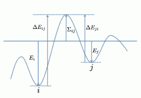
Figure 1: Potential energy landscape description. Energies $E_{i}$ are measured positive downwards. Energy gaps $\Sigma_{ij}$ are defined positive upwards.

The system under investigation is pictured as a walker exploring the network through a biased random walk. The rate (probability per unit time) $r_{i\to j}$ to go from vertex $i$ to vertex $j$ depends a priori on the energy at vertices $i$ and $j$ and/or the energy barrier between $i$ and $j$ that must be overcome. The random walk model is defined in discrete time $t$ as follows:

• At time $t$, the walker is in vertex $i$.

• It chooses at random a neighbor of $i$, namely $j$.

• With a probability $r_{i\to j}$, that depends on the energy $E_{i}$ and/or on the energy barrier $\Delta E_{ij}$, the walker hops to vertex $j$.

• Time is updated $t\to t+1$.

The relationship between the probabilities $r_{i\to j}$ and the energy and energy barriers can be of different forms. In usual unbiased random walks, $r_{i\to j}$ is a constant independent of both $i$ and $j$ [36]. As a first step to introduce a dependence on the nodes, a possible approach is that in which the energy barriers depend only on the local minima themselves, i.e. we consider $\Sigma_{ij}=0$. For example, in the Bouchaud trap model considered in Ref. [11], the probability to exit from a trap is just an Arrhenius law depending only on the departing trap’s depth, namely

$$r_{i\to j}^{traps}=r_{0}e^{-\beta E_{i}},$$ (1)

where $\beta=1/T$ is the inverse temperature and $r_{0}$ is a constant that determines a global timescale. Other possible definitions include the Metropolis one

$$r_{i\to j}^{Metropolis}=r_{0}\min\left(1,e^{\beta(E_{j}-E_{i})}\right),$$ (2)

and the Glauber rate

$$r_{i\to j}^{Glauber}=\frac{r_{0}}{1+e^{-\beta(E_{j}-E_{i})}}.$$ (3)

We note that the rates considered in the Bouchaud trap model are quite different from the Metropolis or Glauber rates. Indeed, while the former depends only on the depth of the originating trap, the latter depend also on the energy of the arriving vertex. This translates in the fact that, in the limit of zero temperature, the dynamics of the Bouchaud trap model is frozen for any $E_{i}$, while Metropolis and Glauber dynamics still allow jumps to lower energy minima [13]. Within an even more realistic representation of glassy dynamics, one can also contemplate the case $\Sigma_{ij}\neq 0$, allowing for the transition rates to depend explicitly on the energy barriers between adjacent minima. As a paradigm of this choice, we propose a rate of the Arrhenius form

$$r_{i\to j}^{barriers}=r_{0}e^{-\beta\Delta E_{ij}},$$ (4)

which acts a straightforward generalization of the local transition rate (1).

The case of rate (1) (local trapping) was studied in a previous publication [34]. In the following, we will consider in turn non-local rates (2), (3) and (4) and discuss the fundamental differences due to the introduction of energy barriers in the model.

We emphasize that our model differs both from usual unbiased random walks, as the local energy determines the transition rates, and from mean-field trap models in which jumps between any pair of energy minima are a priori possible: Here, the system can jump only between neighboring nodes. The dynamical evolution depends therefore both on the network topology and on the energies associated to the nodes.

2.2 Numerical implementation

To implement numerically the random walk, it is convenient to resort to the techniques developed for general diffusion processes on complex weighted networks [37]. The main advantage of this method is to avoid rejection steps, thus improving dramatically the computational efficiency [38, 39]. Therefore, at each simulation step the random walker sitting at node $i$ selects a neighbor $j$ with probability $r_{i\to j}/\sum_{j}r_{i\to j}$, where the sum in the normalizing factor is extended to all of $i$’s neighbors. As the walker hops on node $j$, the physical time is incremented by an interval $\Delta t$ drawn from the exponential distribution $P(\Delta t)=1/\overline{\Delta t}\exp(-\Delta t/\overline{\Delta t})$, where $\overline{\Delta t}=k_{i}/\sum_{j}r_{i\to j}$ is the inverse of the average escape rate out of node $i$. In this way the simulation time is disentangled from the physical time and the latter has no impact on the simulation efficiency. No matter how much physical time a walker spends in a node, from the simulation time point of view it is always just a time step.

The network substrates on which we will focus are scale-free networks with a degree distribution of the form $P(k)\sim k^{-\gamma}$ and $2<\gamma\leq 3$. We will generate them with the Uncorrelated Configuration Model (UCM) [40], that allows us to tune the degree distribution to the desired form and prevents the formation of degree-degree correlations. Networks are therefore generated as follows: A number of stubs (or semi-links) extracted from the desired final degree distribution is assigned to each node. Stubs are then randomly paired to form links between nodes, with the prescription that multiple links as well as self-loops must be avoided. A minimal degree $m$ is fixed a priori. To avoid spurious effects due to the possible presence of tree-like structures [41] it is convenient to adopt $m>2$. We will choose $m=4$ in all of our simulations. So far the algorithm coincides with the one of the Configuration Model [42], but the UCM introduces moreover a cutoff to the degree distribution, $k_{c}=N^{1/2}$, which avoids the formation of degree correlations by limiting the size of the hubs [40].

3 Heterogeneous mean-field theory

In order to gain analytical understanding of the role of the different transition rates in the corresponding glassy dynamics, we apply a standard heterogeneous mean-field (HMF) formalism [6, 35] . The basic tenet of HMF is the assumption that all the dynamical properties of a vertex depend only on its degree. Vertices are thus grouped into classes according to their degree, and vertices with the same degree are treated as equivalent. This approximation is consistent with previous findings that have uncovered the correlations between the energy of a local minimum and the degree of the corresponding node in the network [25]. We therefore make the assumption that there exists a relationship $E_{i}=h(k_{i})$ where the function $h(k)$ is a characteristic of the model. This also means that the distributions of energies $\rho(E)$ of the system’s landscape, and the degree distribution $P(k)$ of the corresponding network are linked through $h$. In the same spirit, we make the further assumption that the energy gap between minima $i$ and $j$ depends only on the degrees of $i$ and $j$, i.e., that it can be written as $\Sigma_{i,j}=\sigma(k_{i},k_{j})$, where $\sigma(k,k^{\prime})$ is a symmetric function of $k$ and $k^{\prime}$.

Under the HMF approximation the dynamics will thus focus on the transitions between different degree classes. The rate to go from a vertex $k$ to a vertex $k^{\prime}$ can be written as

$$W_{kk^{\prime}}=P(k^{\prime}|k)r(k\to k^{\prime}).$$ (5)

The function $P(k^{\prime}|k)$, defined as the conditional probability that a vertex of degree $k$ is connected with another vertex of degree $k^{\prime}$ [43], takes into account the topological features of the network, by gauging the probability of selecting a vertex $k^{\prime}$ as neighbor of $k$. The function $r(k\to k^{\prime})$ measures the rate of jumping from a vertex of degree $k$ to a vertex of degree $k^{\prime}$ (given that they are connected by an edge), and depends on $k$ and $k^{\prime}$ through the rates $r_{i\to j}$ and the functions $h$ and $\sigma$. Obviously, the rate $r(k\to k^{\prime})$ is not in general a symmetric function of $k$ and $k^{\prime}$. It is worth noting that, apart from a normalization, Equation (5) is simply the so-called weighted propagator describing the probability that a node in class $k$ interacts with a node in class $k^{\prime}$ [37]. We also note that the rates $r(k\to k^{\prime})$ depend on the inverse temperature $\beta$ through the microscopic rates $r_{i\to j}$.

4 General HMF formalism

In this section, we apply the HMF theory to compute different quantities relevant for the characterization of the dynamics of a random walk in a complex energy landscape represented in terms of a network of minima.

4.1 Occupation probability

The description of a random walk dynamics starts from the occupation probability $P(k,t_{w})$, defined as the probability for the walker to be in any node of degree $k$ at a time $t_{w}$. Its time evolution can be easily represented in terms of a master equation of the form

$$\frac{\partial P(k,t_{w})}{\partial t_{w}}\equiv\dot{P}(k,t_{w})=-\sum_{k^{\prime}}W_{kk^{\prime}}P(k,t_{w})+\sum_{k^{\prime}}W_{k^{\prime}k}P(k^{\prime},t_{w}).$$ (6)

Upon describing the state at time $t_{w}$ with the row vector ${\bf P}(t_{w})=\left\{P(1,t_{w}),P(2,t_{w}),\!...\!,P(k_{c},t_{w})\right\}$, where $k_{c}$ is the cutoff or largest degree in the network, Equation (6) can be rewritten in vector form as

$$\dot{\bf P}(t_{w})=-{\bf P}(t_{w})L\ ,$$ (7)

where the matrix $L$, with elements

$$L_{k^{\prime}k}=\left(\delta_{k^{\prime}k}\sum_{l}W_{kl}-W_{k^{\prime}k}\right)\ ,$$ (8)

is a generalization of a Laplacian matrix to the case of directed weighted graphs. The matrix elements satisfy

$$L_{k^{\prime}k^{\prime}}=\sum_{k,k\neq k^{\prime}}L_{k^{\prime}k}\ ,$$ (9)

which ensures conservation of probability and states that the columns of $L$ are not linearly independent. The real part of every eigenvalue of $L$ is non-negative [44]. As a consequence, all solutions of Eq. (7), which can be formally written as

$${\bf P}(t_{w})={\bf P}(t_{0})e^{-L(t_{w}-t_{0})}\ ,$$ (10)

are stable according to Lyapunov criteria. In particular, since $\det L=0$, $L$ always has the eigenvalue $0$, which corresponds to a constant solution of the problem. At this point one can proceed in close analogy with discrete-time regular Markov chains [45]. By making the assumption that the matrix $W_{k^{\prime}k}$ is non-negative and irreducible (indeed it is for every choice of $r(k^{\prime}\rightarrow k)$ in the following), we can prove that the $0$ eigenvalue of $L$ has algebraic multiplicity $1$. Hence, the stationary solution of Eq. (7) is unique.

4.1.1 Steady state

In order to calculate the steady solution ${\bf P}^{\infty}$ in the limit $t_{w}\to\infty$, one can impose $\dot{\bf P}(t_{w})=0$. This leads to the condition

$${\bf P}^{\infty}L=0,$$ (11)

so that we are left with the task of finding the left nullspace of $L$. Eq. (11) is a homogeneous system of algebraic linear equations. It admits non-trivial solutions since $\det(L)=0$. In our case, the solution to (11) can be easily found by imposing the detailed balance condition. Namely, writing Eq. (11) as

$$\sum_{k^{\prime}}\left[-W_{kk^{\prime}}P^{\infty}(k)+W_{k^{\prime}k}P^{\infty}(k^{\prime})\right]=0,$$ (12)

we can obtain a solution by imposing that the terms inside the summation in Eq. (12) cancel individually, that is

$$W_{kk^{\prime}}P^{\infty}(k)=W_{k^{\prime}k}P^{\infty}(k^{\prime}),\qquad\forall k,k^{\prime}.$$ (13)

Substituting the form of $W_{kk^{\prime}}$, we obtain

$$\frac{P^{\infty}(k)}{P^{\infty}(k^{\prime})}=\frac{W_{k^{\prime}k}}{W_{kk^{\prime}}}=\frac{P(k|k^{\prime})r(k^{\prime}\to k)}{P(k^{\prime}|k)r(k\to k^{\prime})}=\frac{kP(k)}{k^{\prime}P(k^{\prime})}\frac{r(k^{\prime}\to k)}{r(k\to k^{\prime})},$$ (14)

where in the last step we have used the degree detailed balance condition $kP(k)P(k^{\prime}|k)=k^{\prime}P(k^{\prime})P(k|k^{\prime})$ which simply expresses that the number of edges from a node of degree $k$ to a node of degree $k^{\prime}$ is equal to the number of edges from a node of degree $k^{\prime}$ to a node of degree $k$ [46]. From Eq. (14), we see that its right-hand-side must be expressible as a simple ratio of a function of $k$ over a function of $k^{\prime}$. A general way to obtain this is to impose a coarse-grained rate $r(k^{\prime}\rightarrow k)$ taking the general form

$$r(k^{\prime}\rightarrow k)=f(k^{\prime})g(k)s(k^{\prime},k).$$ (15)

In other words, we assume that the rate $r(k^{\prime}\rightarrow k)$ can be written as the product of a function of $k^{\prime}$, a function of $k$, and a symmetric function $s(k^{\prime},k)=s(k,k^{\prime})$ (where $k$ and $k^{\prime}$ need not be separable). We will see later that all the rates $r_{i\to j}$ defined in Sec. 2.1 (traps, Glauber, Metropolis, and energy barriers) can be written in such a form. The stationary solution is then given by

$$P^{\infty}(k)=\frac{1}{\mathcal{Z}}kP(k)g(k)/f(k)$$ (16)

where ${\mathcal{Z}}$ is a normalizing constant determined by the condition $\sum_{k}P^{\infty}(k)=1$. Such a solution is unique, as proven above. Interestingly, the symmetric function $s(k^{\prime},k)$ does not enter the steady solution, although it will play a role in affecting the transient behavior, as we will see in the next sections.

4.1.2 Glassy phase

The steady state solution found above for the occupation probability is defined if and only if the normalization constant

$$\mathcal{Z}=\sum_{k}kP(k)g(k)/f(k).$$ (17)

is finite. When this condition is met, the random walker reaches an equilibrium state with a distribution ${\bf P}^{eq}={\bf P}^{\infty}$. On the other hand, whenever such condition is not met, the random walker is unable to reach a steady state, i.e. the steady solution to the rate equation does not correspond to any physical steady state in equilibrium ${\bf P}^{eq}$. We identify this region of the phase space with the glass phase for our random walker [11].

The functions $f$ and $g$ depend on the temperature, on the precise dynamics chosen (traps, Glauber, Metropolis), and encode the relationship $h$ between energy and degree of the minima. The degree distribution moreover enters explicitly the expression $\mathcal{Z}$. As the various parameters of the model are changed, it is thus a priori possible to go from one phase in which $\mathcal{Z}$ is finite to one in which $\mathcal{Z}$ diverges. In a physical system in particular, the control parameter is usually the temperature, while the topology of the network of minima and the function $h$ are given. It is then clear from Eq. (17) that the presence or absence of a finite glass transition temperature $\beta_{c}$, such that $\mathcal{Z}$ becomes infinite for $\beta\geq\beta_{c}$, depends on the interplay between the topology of the landscape network (as determined by $P(k)$) and the functions $f$ and $g$. Interestingly, at this mean-field level, the existence of a transition does not depend on the network degree correlations, since the conditional probability $P(k^{\prime}|k)$ do not enter Eq. (17).

Let us consider for instance a network of minima with a heavy-tailed degree distribution such as $P(k)\sim k^{-\gamma}$. A transition between a finite and an infinite $\mathcal{Z}$ can be observed if and only if $g(k)/f(k)$ behaves at large $k$ in the form $\sim k^{a}$ where the exponent $a$ depends on the temperature, and can take values smaller or larger than $\gamma-2$ depending on the temperature. Another example is given by a stretched exponential form for $P(k)$, $P(k)\sim e^{-bk^{a}}$, in which case a transition is observed if and only if $g(k)/f(k)$ is of the form $e^{b^{\prime}k^{a}}$, with $b^{\prime}$ a function of the temperature (the transition is then given by $b^{\prime}(\beta_{c})=b$).

4.1.3 Glassy dynamics

In any finite system, unless the product function $g(k)/f(k)$ exhibits some sort of singularity, the normalization constant Eq. (17) is finite and the steady state distribution $P^{\infty}(k)$ exists, the occupation probability $P(k,t_{w})$ converging to it after an equilibration time, i.e.

$$\lim_{t_{w}\to\infty}P(k,t_{w})=P^{\infty}(k).$$ (18)

The corresponding thermalization of the occupation probability occurs in a way depending on the function $h$. Shallow energy minima are indeed explored first, while deep traps (large $E$) are visited at larger times [11, 13]. If $h$ is a growing function of $k$, as indeed found empirically [25], small degree nodes correspond to shallow minima, and deeper minima are associated to larger nodes. The evolution of $P(k,t_{w})$ takes then place in a hierarchical fashion: The small degree region equilibrates first, and progressive equilibration of larger degree regions takes place at larger times. In this respect, we obtain a strong difference between the biased random walk that the glassy system experiences and usual diffusion processes corresponding to unbiased random walks, which visit first large degree vertices and then cascade down towards small degree nodes [36, 47, 6], in the present case we observe an “inverse cascade process” from small vertices to hubs.

We have found in [34] that, in the case of a random walk among traps, this hierarchical thermalization is summarized in a scaling form for $P(k,t_{w})$, which can be written as

$$P(k,t_{w})=k_{w}(t_{w})^{-1}\mathcal{F}\left(\frac{k}{k_{w}(t_{w})}\right),$$ (19)

where $k_{w}(t_{w})$ represents the maximum degree of the vertices equilibrated up to time $t_{w}$, and $\mathcal{F}(x)$ interpolates between $P^{\infty}(x)$ at small $x$ and the short time form of $P(k,t_{w})$ which is proportional to $kP(k)$. We will see in the next section that a similar scaling is obeyed for other transition rates. In general, for the glassy dynamics, the functional form of $k_{w}(t_{w})$ can moreover be obtained through the following argument: The total time $t_{w}$ can be written as the sum of the trapping times spent in the vertices that have been visited since the beginning of the dynamics. Trapping times increase with the depth of the minimum, hence with the degree (we are still considering the case of an increasing function $h(k)$), and, in the glassy phase, the consequence is that the sum of trapping times is dominated by the vertex with the largest degree visited up to that point, namely $k_{w}$. Moreover, the average trapping time $\tau_{k}$ at a given vertex $k$ can be estimated as the inverse of the average escape rate $r_{k}$ from that vertex:

$$\frac{1}{\tau_{k}}=r_{k}=\sum_{k^{\prime}}W_{kk^{\prime}}=\sum_{k^{\prime}}P(k^{\prime}|k)r(k\to k^{\prime})=\sum_{k^{\prime}}P(k^{\prime}|k)f(k)g(k^{\prime})s(k,k^{\prime}).$$ (20)

We can therefore estimate $k_{w}(t_{w})$, the typical degree up to which nodes are “equilibrated” at time $t_{w}$, by approximating $\tau_{k_{w}}\sim t_{w}$, and solving the equation

$$t_{w}=\frac{1}{f(k_{w})}\frac{1}{\sum_{k^{\prime}}P(k^{\prime}|k_{w})g(k^{\prime})s(k^{\prime},k_{w})}$$ (21)

to obtain $k_{w}$ as a function of $t_{w}$. Note that the result depends here on the function $s(k,k^{\prime})$ and not only on $f$, $g$, $h$ and $P(k)$.

4.2 Average escape time

The properties of the system can be further quantified by measuring the average time $t_{esc}(t_{w})$ required by the random walker to escape from the vertex it occupies at time $t_{w}$ [34]. For small waiting times $t_{w}$, $t_{esc}$ increases as a result of the transient equilibration of $P(k,t)$. For large $t_{w}$, such that $P(k,t_{w})$ is close enough to the equilibrium $P^{\infty}$, $t_{esc}$ can be calculated instead as the average

$$t_{esc}(t_{w}\to\infty)=\sum_{k}P^{\infty}(k)\tau_{k}=\frac{1}{\mathcal{Z}}\sum_{k}kP(k)[g(k)/f(k)]\tau_{k}$$ (22)

where $\tau_{k}=1/r_{k}$ is the inverse of the equilibrium escape rate, cf Eq. (20), yielding

$$t_{esc}(t_{w}\to\infty)=\frac{1}{\mathcal{Z}}\sum_{k}\frac{kP(k)g(k)}{f(k)^{2}\sum_{k^{\prime}}P(k^{\prime}|k)g(k^{\prime})s(k^{\prime},k)}.$$ (23)

Most interestingly, the explicit form of the average escape time $t_{esc}$ depends explicitely on the symmetric function $s(k,k^{\prime})$ as well as on the network degree correlations, as expressed by the conditional probability $P(k^{\prime}|k)$.

4.3 Average rest time

Let us go back to the issue of the existence of a glass transition in the model. We first recall the phenomenology of the fully connected trap model, with transition rates $r_{i\to j}=r_{0}e^{-\beta E_{i}}/N$ for any $i$ and $j$, where the energies $E_{i}$ are random numbers extracted from a distribution $\rho(E)$ [11, 14]. As all traps are connected with each other, all traps are equiprobable after a jump, so that the probability for the system to be in a trap of depth $E$ is simply $\rho(E)$, and the average rest time spent in a trap is $\langle\tau\rangle=\int\rho(E)e^{\beta E}dE$. A transition between a high temperature phase and a glassy one is thus obtained if and only if, when $\beta$ increases, $\langle\tau\rangle$ is finite at small $\beta$ and diverges at a finite $\beta_{c}$. Such a phenomenology is obtained if and only if $\rho(E)$ is of the form $\exp(-\beta_{c}E)$ at large $E$ (else the transition temperature is either $0$ or $\infty$), and the transition temperature is then $T_{c}=1/\beta_{c}$ [11].

In the present case of a nework of minima, the average rest time that the walker spends in a minimum is

$$\langle\tau\rangle=\left\langle\frac{1}{r_{k}}\right\rangle_{h},$$ (24)

where the symbol $\langle...\rangle_{h}$ refers to the average performed over the measure $P_{h}(k)$, which represents the probability that the walker is in any vertex of degree $k$ after a hop. Note that we disregard here the physical time, which is the sum of times spent in the various minima, but consider only the number of hops between minima. In the case of the traps model, $P_{h}$ is simply given by the probability to be in a node of degree $k$ after a hop in a random walk, i.e. by $kP(k)/\langle k\rangle$ [34], since the transition rates do not depend on the arrival node. In a non-local trapping model instead, we need to write a master equation of the form

$$\dot{P}_{h}(k)=-P_{h}(k)+\sum_{k^{\prime}}\mathcal{W}_{k^{\prime}k}P_{h}(k^{\prime}),$$ (25)

where the matrix $\mathcal{W}_{k^{\prime}k}=W_{k^{\prime}k}/\sum_{l}W_{k^{\prime}l}=W_{k^{\prime}k}/r_{k^{\prime}}$ is now stochastic and the derivative is intended with respect to the number of hops. In the long time limit, we impose $\dot{P}_{h}(k)=0$ and calculate $P_{h}(k)$ as we did for $P^{\infty}(k)$, imposing the detailed balance condition, and obtaining

$$P_{h}(k)=\frac{1}{\mathcal{I}}kP(k)[g(k)/f(k)]r_{k}\ ,$$ (26)

where $\mathcal{I}$ is a normalization factor, given by

$$\mathcal{I}=\sum_{k}\sum_{l}kP(k)P(l|k)g(k)g(l)s(k,l).$$ (27)

We finally obtain for the average $\langle\tau\rangle$:

$$\langle\tau\rangle=\sum_{k}P_{h}(k)/r_{k}=\frac{\mathcal{Z}}{\mathcal{I}},$$ (28)

where $\mathcal{Z}$ is the normalization factor of $P^{\infty}(k)$ defined in Eq. (17). As for the average escape time, the average rest time $\langle\tau\rangle$ thus depends on all the parameters of the system, including the network’s degree correlations and the symmetric function $s$.

5 Application to physical transition rates

In this section, we apply the general HMF results obtained in the previous section to physical transition probabilities between local minima given by the trap model, Glauber, Metropolis and barrier-mediated rates. We will focus for definiteness on scale-free networks characterized by a power-law degree distribution $P(k)\sim k^{-\gamma}$ with $2<\gamma\leq 3$, which turns out to be the interval reported in the literature [23, 25].

Let us first consider the explicit form of the transition rates in each case, to show that they can be cast in the form given by Eq. (15). In the case of the trap model, the rate to jump from a vertex $k$ to a vertex $k^{\prime}$ is simply $r(k\to k^{\prime})=r_{0}e^{-\beta E_{k}}=r_{0}e^{-\beta h(k)}$, where we recall that $h(k)$ gives the depth of a node of degree $k$: it depends only on the degree of the starting node, and not on the node reached after the jump. We can therefore use

$$\mbox{(Trap model)}\quad f(k)=e^{-\beta h(k)},\;\;g(k)=1,\;\;s(k,k^{\prime})=r_{0}.$$ (29)

The Glauber rate can be written as

$$r(k\rightarrow k^{\prime})=r_{0}\frac{e^{\beta h(k^{\prime})}}{e^{\beta h(k)}+e^{\beta h(k^{\prime})}},$$ (30)

leading to

$$\mbox{(Glauber)}\quad f(k)=1,\;\;g(k)=e^{\beta h(k)},\;\;s(k,k^{\prime})=r_{0}\frac{1}{e^{\beta h(k)}+e^{\beta h(k^{\prime})}}.$$ (31)

The Metropolis transition, on its turn, reads

$$r(k\rightarrow k^{\prime})=r_{0}\min\left[1,e^{\beta(h(k^{\prime})-h(k))}\right].$$ (32)

Since, for positive $a$, $\min(1,b/a)=\min(a,b)/a$, we can choose

$$\mbox{(Metropolis)}\;f(k)=e^{-\beta h(k)},\;g(k)=1,\;s(k,k^{\prime})=r_{0}\min(e^{\beta h(k)},e^{\beta h(k^{\prime})}).$$ (33)

Finally, in the presence of energy barriers, the transition rate reads

$$r(k\to k^{\prime})=r_{0}e^{-\beta(h(k)+\sigma(k,k^{\prime}))},$$ (34)

where $\sigma(k,k^{\prime})$ is a symmetric function of its arguments, so that we can use

$$\mbox{(Barriers)}\;f(k)=e^{-\beta h(k)},\;g(k)=1,\;s(k,k^{\prime})=r_{0}e^{-\beta\sigma(k,k^{\prime})}.$$ (35)

5.1 Steady state and the glass transition temperature

Interestingly, for all the transition rates considered above, the product of the functions $1/f$ and $g$, which controls the existence of the steady state solution of the occupation probability, takes the form

$$g(k)/f(k)\equiv e^{\beta h(k)}.$$ (36)

The normalization constant $\mathcal{Z}$ defined in Eq. (17) can thus be written as

$$\mathcal{Z}=\sum_{k}kP(k)e^{\beta h(k)}.$$ (37)

For a power-law degree distribution $P(k)\sim k^{-\gamma}$, a finite glass transition temperature is then obtained if and only if $h$ is of the form

$$h(k)=E_{0}\log(k)\ ,$$ (38)

which is precisely what has been found, in conjunction with a scale-free degree distribution, in Ref. [25]. $\mathcal{Z}$ is then indeed given by a sum of terms of the form $k^{1-\gamma+\beta E_{0}}$, which converges if and only if

$$\beta E_{0}-\gamma<-2\ .$$ (39)

In other words, a transition between a high temperature phase in which $P^{\infty}(k)$ exists and a low temperature glassy phase is obtained at the critical temperature [34]

$$T_{c}=\frac{1}{\beta_{c}}=\frac{E_{0}}{\gamma-2}\ .$$ (40)

Quite noticeably, the existence of a transition at a finite temperature, as well as the value of this temperature, does not depend on the form of the transition rates between the local minima, but only on the existence of a particular interplay between the topology of the network of minima and the relationship between energy and degree in this network, as determined by the function $h$. We emphasize that this result is also independent of the network degree correlations $P(k^{\prime}|k)$, as already noted in the previous section.

5.2 The steady state and finite size effects

Let us focus on the case of a scale-free network of minima, with $P(k)\propto k^{-\gamma}$ and $E_{i}=E_{0}\log(k_{i})$. For any of the rates discussed above, the steady state measure, when it exists, is given by

$$P^{\infty}(k)=\frac{k^{1-\gamma+\beta E_{0}}}{\zeta(-1+\gamma-\beta E_{0})}\;\mbox{for}\;\gamma-\beta E_{0}>2,$$ (41)

where $\zeta$ is the Riemann $\zeta$ function. A plot of $P^{\infty}(k)$ as a function of $k$ and $\gamma-\beta E_{0}$ is given in Fig. 2, while data from simulations are reported in Fig. 3 for the evolution of $P(k,t_{w})$ under Glauber dynamics. Above the transition ($\gamma-\beta E_{0}>2$), low-$k$ states (i.e., shallow minima) are more probable. As the temperature decreases, $P^{\infty}(k)$ becomes less and less peaked at low values of $k$, and large-$k$ states, which correspond to lower energies, become more and more probable.

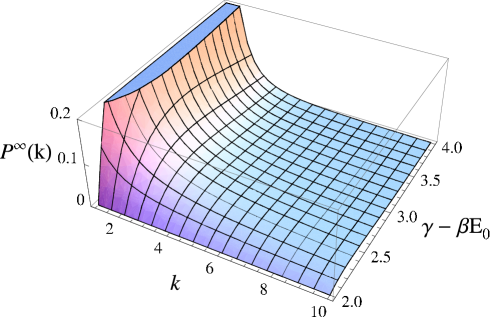
Figure 2: Equilibrium probability distribution $P^{\infty}(k)$ for the random walker to be in any node of degree $k$. For $\gamma-\beta E_{0}=2$ the system undergoes a transition to a glassy state.

In any finite system, the sum defining $\mathcal{Z}$, is finite at any temperature as the degree distribution has a cut-off at a finite $k_{c}$:

$$\mathcal{Z}=\sum_{k}^{k_{c}}kP(k)g(k)/f(k).$$ (42)

For instance, for $P(k)\propto k^{-\gamma}$, and with $h(k)=E_{0}\log(k)$, the sum

$$\sum_{k=1}^{k_{c}}k^{1-\gamma+\beta E_{0}}=H_{k_{c}}^{(-1+\gamma-\beta E_{0})}$$ (43)

is analytic in $\gamma-\beta E_{0}=2$ for any finite $k_{c}$. Here $H_{k_{c}}^{(\alpha)}$ is the Harmonic Number of order $\alpha$, which tends to $\zeta(\alpha)$ for $k_{c}\to\infty$.

The probability $P^{\infty}(k)$ is thus well defined for every $\gamma-\beta E_{0}$ and for any finite system. In particular, performing a continuous degree approximation in Eq. (43), we can obtain an estimate of the network size dependence of $\mathcal{Z}$ as

$$\mathcal{Z}\sim\int^{k_{c}}k^{1-\gamma+\beta E_{0}}\;dk\sim\mbox{const}+k_{c}^{2-\gamma+\beta E_{0}}.$$ (44)

For $\beta<(\gamma-2)/E_{0}$, $\mathcal{Z}$ tends to a constant as the network size (and thus $k_{c}$) increases. On the other hand, for $\beta>(\gamma-2)/E_{0}$, $\mathcal{Z}$ diverges as $k_{c}^{2-\gamma+\beta E_{0}}$, i.e., as $N^{(2-\gamma+\beta E_{0})/2}$ in uncorrelated scale-free networks, which obey $k_{c}\sim N^{1/2}$.

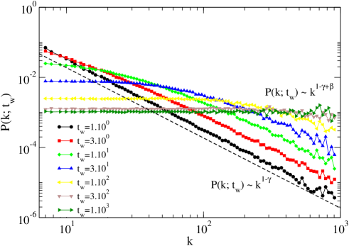
Figure 3: Evolution towards equilibrium of the probability distribution $P(k;t_{w})$ for Glauber dynamics. The distribution measured after a small waiting time $t_{w}$ is determined by a usual unbiased random walk behavior, i.e $P(k;t_{w})\sim kP(k)$, while at larger times it relaxes to the equilibrium $P^{\infty}(k)$. The relaxation towards equilibrium starts from small degree nodes. Data refer to UCM networks with $N=10^{6}$ and $\gamma=3.0$ for $\beta=2$ ($E_{0}=1$): with these parameter values, for small times $P(k;t_{w})\sim k^{-2}$, while at large enough times $P(k;t_{w})\sim P^{\infty}(k)=const$.

5.3 Glassy dynamics

At low temperatures, even for a finite system, the evolution of $P(k;t_{w})$ towards $P^{\infty}(k)$ is slow, as displayed in Fig. 3, and an ageing regime takes place, in which the function $P(k,t_{w})$ obeys the scaling form

$$P(k,t_{w})=k_{w}(t_{w})^{-1}\mathcal{F}\left(\frac{k}{k_{w}(t_{w})}\right),$$ (45)

where the characteristic degree $k_{w}$ can be estimated from Eq. (21). In order to simplify its computation, we will consider an uncorrelated network of minima, such that $P(k^{\prime}|k)=k^{\prime}P(k^{\prime})/\langle k\rangle$, and we will work in the continuous degree approximation, using the normalized form $P(k)=(\gamma-1)m^{\gamma-1}k^{-\gamma}$, where $m$ is the minimum degree present in the network.

In the case of the Glauber dynamics, the escape rate can be expressed, within the above approximations, as

$$r_{k} = \frac{1}{\langle k\rangle}\int_{m}^{\infty}k^{\prime}P(k^{\prime})r_{0}\frac{e^{\beta h(k^{\prime})}}{e^{\beta h(k)}+e^{\beta h(k^{\prime})}}\;dk^{\prime}\equiv\frac{m^{\gamma-1}(\gamma-1)}{\langle k\rangle}\int_{m}^{\infty}\frac{z^{1+E_{0}\beta-\gamma}}{z^{E_{0}\beta}+k^{E_{0}\beta}}dz$$ (46)

$$= \Gamma\left[1,\frac{\gamma-2}{\beta},1+\frac{\gamma-2}{\beta},-\left(\frac{k}{m}\right)^{\beta}\right],$$

where we have used the relation $h(k)=E_{0}\ln k$ and where $\Gamma[a,b,c,z]$ is the Gauss Hypergeometric function. Using the asymptotic expansion for $z\to 0$ [48], we obtain that the leading behavior for large $k$ yields

$$r_{k}\sim\left\{\begin{array}[]{lr}k^{-\beta_{c}E_{0}}&\beta>\beta_{c}\\ k^{-\beta E_{0}}&\beta<\beta_{c}\\ \end{array}\right.,$$ (49)

which leads to

$$\tau_{k}=\frac{1}{r_{k}}\sim\left\{\begin{array}[]{lr}k^{\beta_{c}E_{0}}&\beta>\beta_{c}\\ k^{\beta E_{0}}&\beta<\beta_{c}.\\ \end{array}\right..$$ (52)

From here, using the relation $\tau_{k_{w}}\sim t_{w}$, we obtain

$$k_{w}\sim\left\{\begin{array}[]{lr}t_{w}^{1/(\beta_{c}E_{0})}&\beta>\beta_{c}\\ t_{w}^{1/(\beta E_{0})}&\beta<\beta_{c}.\\ \end{array}\right..$$ (55)

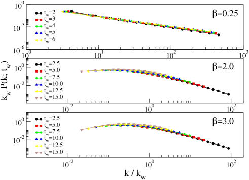
Figure 4: Data collapse for the time evolution of the occupation probability $P(k;t_{w})$ at different temperatures (Glauber dynamics). Data refer to UCM networks with $N=10^{6}$ and $\gamma=2.5$, so that $\beta_{c}=\gamma-2=0.5$ (where we have taken $E_{0}=1$). The top panel presents data for $\beta<\beta_{c}$ while both middle and bottom panels concern the low temperature case $\beta>\beta_{c}$. Accordingly, for the top panel we use $k_{w}\sim t_{w}^{1/\beta}\sim t_{w}^{4}$ for the rescaling, while for the central and the bottom ones it holds $k_{w}\sim t_{w}^{1/\beta_{c}}=t_{w}^{2}$ (see Eq. (55)). The curves corresponding to different $t_{w}$ collapse well under this rescaling. Note that we use rather small values of $t_{w}$, because the equilibration time, defined by $k_{w}\sim k_{c}\sim N^{1/2}$, is $t_{eq}\sim N^{\frac{\beta_{c}}{2}}\simeq 32$ for $\beta>\beta_{c}$ and $t_{eq}\sim N^{\frac{\beta}{2}}\simeq 6$ for $\beta<\beta_{c}$. Each curve is obtained by averaging over $3\times 10^{6}$ simulation runs.

In Fig. 4 we check the validity of Eqs. (45) and (55) by performing a data collapse analysis for different values of $t_{w}$. The curves obtained for different $t_{w}$ collapse indeed as predicted.

In the case of the Metropolis transition rates, a similar analysis yields

$$r_{k}^{Metropolis}\propto\frac{1}{(\beta_{c}-\beta)E_{0}}\left(k^{-\beta E_{0}}-\frac{\beta}{\beta_{c}}k^{-\beta_{c}E_{0}}\right),$$ (56)

leading to the same asymptotic behavior as in Eq. (49), and therefore to the same scaling picture as for the Glauber rate.

As pointed out for the case of the traps model [34], however, in finite systems the scaling relations in Eq. (55) hold only as far as $k_{w}(t_{w})<k_{c}$, i.e. it exists an equilibration time $t_{eq}$, obtained by inverting Eq. (55), above which the system has completely relaxed and Eq. (45) is no more valid. Finally, it is worth stressing that, while for large temperatures the scaling exponent relating $k_{w}$ and $t_{w}$ depends on the temperature, in the low temperature phase it becomes independent, being just proportional to the transition temperature. We note that this saturation of the exponent at $1/(\beta_{c}E_{0})$ is very different from the phenomenology obtained in the trap model [34], for which $k_{w}\sim t_{w}^{1/(\beta E_{0})}$. An immediate consequence is that the equilibration time strongly depends on $\beta$, as $t_{eq}\sim k_{c}^{(\beta E_{0})}$, for a system described by traps, but is given by $t_{eq}\sim k_{c}^{(\beta_{c}E_{0})}\ll k_{c}^{(\beta E_{0})}$ for any $\beta>\beta_{c}$ for Glauber and Metropolis rates.

Contrarily to results for the glass transition temperature $T_{c}$ and the steady state, the glassy dynamics for barrier-mediated rates does not yield the same results as for Glauber and Metropolis rates, since $r_{k}$ does depend on the symmetric function $\sigma(k,k^{\prime})$. In particular, we need here to choose a functional form for $\sigma$. We propose to use

$$\sigma(k,k^{\prime})=\sigma_{0}(k^{\mu}+k^{\prime\mu}),$$ (57)

which will be justified in Section 6. In this case we obtain

$$r_{k}^{barriers}\propto r_{0}k^{-\beta E_{0}}e^{-\beta\sigma_{0}k^{\mu}}.$$ (58)

In order to keep an interesting phenomenology, the constant $\sigma_{0}$ cannot be chosen arbitrarily. If $\sigma_{0}$ were independent of the system size, the escape rate would be dominated by the exponential at all temperatures. This behavior would reflect the fact that in this case the rate is suppressed in transitions involving nodes of large $k$, eventually generating unphysically large barriers at large $k_{c}$. To prevent the system from building up infinite barriers, one can impose

$$E_{0}\ln k_{c}\propto\sigma_{0}k_{c}^{\mu},$$ (59)

such that the maximum barrier is always comparable to the lowest energy minimum and neither term dominates the other. As a consequence, we take

$$\sigma_{0}=\epsilon E_{0}\frac{\ln k_{c}}{k_{c}^{\mu}},$$ (60)

where $\epsilon$ is now constant and size independent. Contrarily to the previous cases, $k_{w}(t_{w})$ is hard to determine, as no explicit inversion of Eqs. (21) and (58) can be provided for the range of parameters of interest in our study. A numerical evaluation of $k_{w}(t_{w})$, is reported in Figure 5. The maximum degree of equilibrated vertices $k_{w}$ has an initial power law increase in time, which is reminiscent of the local trapping model. However, as larger degree nodes are equilibrated, exponential barriers come into play and the hierarchical thermalization becomes logarithmic in time.

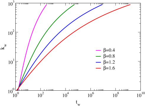
Figure 5: Maximum degree of equilibrated nodes up to time $t_{w}$ for barrier-mediated dynamics. Curves are obtained from the numerical inversion of Eq. (21). Values of parameters are: $\gamma=2.5$, $\beta_{c}=0.5$, $E_{0}=\epsilon=1$, $k_{c}=10^{3}$, $\mu=0.5$.

5.4 Average escape time

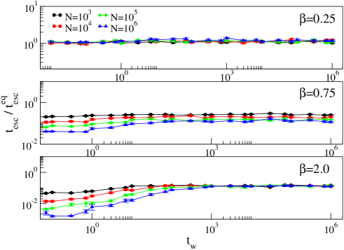
Figure 6: Rescaled average escape times (Metropolis dynamics). Data for UCM network with $\gamma=3.0$, so that $\beta_{c}=1.0$ ($E_{0}=1$). The scaling forms of Eq. (64) produce a collapse of the curves concerning different systems sizes in the three regimes of high, intermediate and low temperature (top, center and bottom panels, respectively). The slightly worse collapse obtained for $\beta=0.75$ may be due to logarithmic corrections as $\beta$ is close to both $\beta_{c}$ and $2\beta_{c}$. Each point is averaged over $400$ simulation runs ($20$ runs on each of $20$ network realizations).

The average escape time, defined as the average time required by the system to escape from the vertex it occupies, can be computed in the long time limit from Eq. (22), as a function of the average trapping time $\tau_{k}$ in vertices of degree $k$. From the asymptotic expansions of $\tau_{k}$ in Eq. (52), valid for Glauber and Metropolis dynamics, evaluation of Eq. (22) allows us to observe that, whenever a finite $T_{c}$ exists, $t_{esc}(t_{w}\to\infty)$ diverges at $2T_{c}$ in an infinite system, as was already observed in the case of local trapping [34]. It is noticeable that the same divergence temperature is obtained, as Eq. (22) a priori involves the network’s degree correlations and the function $s$. Within the continuous degree approximation, the divergence of the escape time with the system size follows the scaling laws

$$t_{esc}^{eq}\equiv t_{esc}(t_{w}\to\infty)\sim\int^{k_{c}}P^{\infty}(k)\tau_{k}\sim\left\{\begin{array}[]{lc}k_{c}^{\beta_{c}E_{0}}&\beta>\beta_{c}\\ k_{c}^{(2\beta-\beta_{c})E_{0}}&\beta_{c}/2<\beta<\beta_{c}\\ \mbox{const.}&\beta<\beta_{c}/2\\ \end{array}\right..$$ (64)

As noted in the previous paragraph for the equilibration time, we note that the scaling for $\beta>\beta_{c}$ differs from the form $k_{c}^{\beta E_{0}}$ encountered for local trapping [34]. Figure 6 reports simulation data that confirm the validity of Eq. (64). As the temperature is lowered, the initial transient becomes longer, but for large enough times $t_{w}$ the asymptotic behavior predicted in Eq. (64) is reached, as made clear from the collapse of curves concerning different system sizes.

In the case of barrier-mediated dynamics, $\tau_{k}$ depends on the symmetric function $\sigma(k,k^{\prime})$, as expressed in Eq. (58), namely

$$\tau_{k}\sim k^{\beta E_{0}}e^{\beta\sigma_{0}k^{\mu}}.$$ (65)

Proceeding as above we obtain

$$t_{esc}\sim\left\{\begin{array}[]{lc}k_{c}^{(1+\epsilon)\beta E_{0}}&\beta>\beta_{c}\\ k_{c}^{[(2+\epsilon)\beta-\beta_{c}]E_{0}}&\beta_{c}/(2+\epsilon)<\beta<\beta_{c}\\ \mbox{const.}&\beta<\beta_{c}/(2+\epsilon)\\ \end{array}\right.,$$ (69)

where we recall that $\epsilon$ does not depend on the system size.

5.5 Average rest time

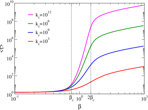
Figure 7: Average rest time for the Glauber dynamics in a scale-free uncorrelated network with $\gamma=2.75$, as a function of the inverse temperature, for different system sizes. Data are obtained by numerical computation of Eq. (28) (with $E_{0}=1$). Note the exponential increase with $\beta$ for $\beta_{c}<\beta<2\beta_{c}$, which saturates for $\beta>2\beta_{c}$ as predicted by Eq. (76).

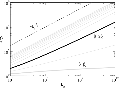
Figure 8: Average rest time for the Glauber dynamics in a scale-free uncorrelated network with $\gamma=2.5$, as a function of the degree distribution cut-off and for different temperatures. Data are obtained by numerical computation of Eq. (28). $\langle\tau\rangle$ grows as a power-law of $k_{c}$, with an exponent that grows as $\beta$ increases (going from bottom to top in the figure). The thick-gray line corresponds to $\beta=\beta_{c}$, while the thick-black line corresponds to $\beta=2\beta_{c}$. For larger values of $\beta$, the power-law behavior corresponds to the predicted $\langle\tau_{k}\rangle\sim k_{c}^{\beta_{c}E_{0}}\sim k_{c}^{\gamma-2}$, which no more depends on $\beta$. The $k_{c}^{\gamma-2}$ curve is reported as a dashed line for reference. Values of $\beta$ represented here are comprised between $0.25$ and $3$.

The HMF expression for the asymptotic average rest time, defined as the average time spent by the system in a minimum, is given by Eq. (28), namely $\langle\tau\rangle=\mathcal{Z}/\mathcal{I}$, where the quantities $\mathcal{Z}$ and $\mathcal{I}$, for uncorrelated scale-free networks and a degree-energy relation $h(k)=E_{0}\ln(k)$, take the form, in the continuous degree approximation,

$$\mathcal{Z} \sim \int^{k_{c}}k^{1-\gamma+\beta E_{0}}\;dk\sim\mbox{const}+k_{c}^{(\beta-\beta_{c})E_{0}},$$ (70)

$$\mathcal{I} \sim \int^{k_{c}}\;dk\int^{k_{c}}\;dk^{\prime}\;k^{1-\gamma}g(k)k^{\prime 1-\gamma}g(k^{\prime})s(k,k^{\prime}).$$ (71)

Let us first recall the case of the local trap model. Both $g(k)$ and $s(k,k^{\prime})$ are then constants, so that $\mathcal{I}\sim\langle k\rangle^{2}=\mathrm{const}$. Thus, the average rest time behaves as $\mathcal{Z}$: it is finite for $\beta<\beta_{c}$, and diverges with the system size as $k_{c}^{(\beta-\beta_{c})E_{0}}$ for $\beta>\beta_{c}$, signaling the emergence of the glassy regime at low temperatures.

In the case of Glauber and Metropolis dynamics (both leading to the same results), the situation is more involved, since the product $g(k)g(k^{\prime})s(k,k^{\prime})$ entering $\mathcal{I}$ is not constant. In fact, $\mathcal{I}$ diverges with $k_{c}$ for $\beta E_{0}>2(\gamma-2)$, that is, at a lower temperature given by $\beta^{\prime}_{c}=2\beta_{c}$. The interplay of these two temperatures determines the behavior of the system for finite sizes within the low temperature phase. In particular, for the Glauber dynamics with $g(k)=e^{\beta h(k)}$ and $s(k,k^{\prime})=r_{0}/[e^{\beta h(k)}+e^{\beta h(k^{\prime})}]$, we have

$$\mathcal{I}\sim\mbox{const}+k_{c}^{(\beta-2\beta_{c})E_{0}}.$$ (72)

Upon considering lower values of $\beta$, $\langle\tau\rangle$ first encounters the divergence of $\mathcal{Z}$ at $\beta_{c}$, which is then partially regularized by the divergence of $\mathcal{I}$ at $2\beta_{c}$. From these results, we obtain the emergence of three scaling regimes for the behavior of $\langle\tau\rangle$ as a function of the system size:

$$\langle\tau\rangle^{\infty}\equiv\langle\tau\rangle(t_{w}\rightarrow\infty)\sim\left\{\begin{array}[]{lc}k_{c}^{\beta_{c}E_{0}}&\beta>2\beta_{c}\\ k_{c}^{(\beta-\beta_{c})E_{0}}&\beta_{c}<\beta<2\beta_{c}\\ \mbox{const.}&\beta<\beta_{c}\\ \end{array}\right..$$ (76)

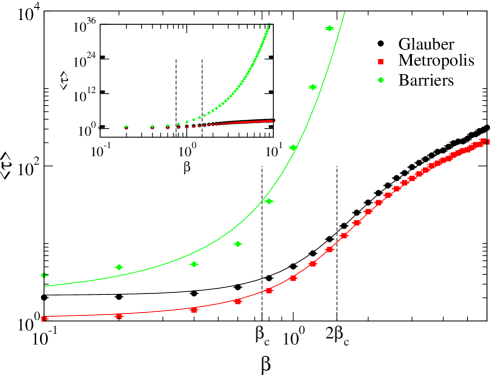
Figure 9: Average rest time as a function of $\beta$ for different transition rates, for a random walker on UCM networks with $\gamma=2.75$ ($E_{0}=1$) and $N=10^{6}$. Discrete points: simulation results; continuous lines: theoretical predictions from $\langle\tau\rangle=\mathcal{Z}/\mathcal{I}$, based on simulation parameters. The Glauber and Metropolis transition rates induce two changes of behavior at $\beta_{c}$ and at $2\beta_{c}$, the first being a steep increase of the average rest time $\langle\tau\rangle$ and the second a smoothing/saturation of this increase. No saturation of $\langle\tau\rangle$ is instead observed when barriers are present. The agreement with theoretical predictions is remarkable, thus corroborating the validity of the HMF assumptions. Moderate deviations are found only in the case of barriers, where exponential growth is expected to add greater fluctuations. In the inset, the difference between the two behaviors is more evident thanks to a different scale of the plot. Note that, since in the simulations $E_{0}=1$, the high temperature limit of the rest time is different for the Glauber and Metropolis dynamics, being $\tau(\beta=0)=2$ and $\tau(\beta=0)=1$ respectively. For the case of barriers we have chosen $\sigma_{0}=10^{-1}$. Each point is obtained by averaging the rest times corresponding to the first $10^{6}$ hops of the random walker in each of $10$ network realizations.

The direct numerical computation of Eq. (28) is shown in Figs. 7 and 8, showing the validity of this analysis. In particular, the exponential increase of $\langle\tau\rangle$ with $\beta$ in the intermediate temperature range $\beta_{c}<\beta<2\beta_{c}$ is clearly apparent in Fig. 7, and Fig. 8 confirms that, for $\beta>2\beta_{c}$, the exponent in the scaling law for the system size $k_{c}$ does not depend on the temperature. While the temperature $\beta_{c}$ signals the onset of the low temperature phase with glassy dynamics for all considered transition rates, for Glauber/Metropolis dynamics the low temperature phase can be further divided into two regions that correspond to different behaviors of the timescales with the system size.

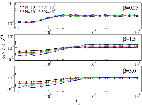
Figure 10: Average rest time for Metropolis dynamics on uncorrelated scale-free networks with $\gamma=3.0$ ($E_{0}=1$, $\beta_{c}=1.0$). Data for different system sizes collapse well when rescaled according to the theoretical values of Eq. (76). While the agreement is excellent both for high and low temperature (top and bottom panels, respectively), logarithmic corrections are probably present for the regime of intermediate temperatures $\beta_{c}<\beta<2\beta_{c}$ (central panel). In each simulation run the rest interval starting before $t_{w}$ and ending after $t_{w}$ is considered, and each point in the Figure is averaged over $400$ simulation runs ($20$ runs on each of $20$ network instances).

Figures 9 and 10 moreover show the result of numerical simulations of random walkers on scale-free networks for Glauber and Metropolis dynamics as well as in the case of barriers, globally confirming the above discussed picture.

Dynamics in the presence of barriers do not yield the same phenomenology as Glauber and Metropolis rate. In this case, we have $g(k)=1$ and $s(k,k^{\prime})=r_{0}e^{-\beta\sigma(k,k^{\prime})}$. Selecting $\sigma(k,k^{\prime})=\sigma_{0}(k^{\mu}+k^{\prime\mu})$, as in Section 5.3, we are led to

$$\mathcal{I}\sim\left[\int^{k_{c}}\;dkk^{1-\gamma}e^{-\beta\sigma_{0}k^{\mu}}\right]^{2}.$$ (77)

As for the escape time $t_{esc}$, upon choosing $\sigma$ size independent, the rest time $\langle\tau\rangle$ will be diverging exponentially with $k_{c}$ at every temperature. By introducing the size dependence as in Eq. (60), instead, one can see that the $\mathcal{I}$ integral converges to a constant for large $k_{c}$ so that one is left with

$$\langle\tau\rangle\sim\left\{\begin{array}[]{lc}k_{c}^{(\beta-\beta_{c})E_{0}}&\beta>\beta_{c}\\ \mbox{const.}&\beta<\beta_{c}\\ \end{array}\right..$$ (80)

We therefore obtain the same picture as in the case of traps, with an exponential increase of $\langle\tau\rangle$ as $\beta$ increases, as confirmed by numerical simulations in Fig. 9.

6 Energy basins and energy barriers

Inspired by analogies with systems governed by the Arrhenius law, we have introduced a transition rate that takes into account the energy barriers between states. Within the heterogeneous mean-field approximation, in which all variables depend only on the degree of the vertices, and choosing $E_{i}=E_{0}\ln(k_{i})$, the transition rate we have considered becomes

$$r(k\rightarrow k^{\prime})=k^{-\beta E_{0}}e^{-\beta\sigma(k,k^{\prime})},$$ (81)

where $\sigma(k,k^{\prime})$ is a symmetric function of the degrees of the two nodes. This model represents in essence an extension of the local trap model, where non-locality enters only in the form of symmetric energy gaps $\Sigma_{ij}$ (see Fig. 1). The steady state has exactly the same form as the ones discussed so far, which incidentally is the same as for the local trap model. As shown in the previous Sections, the presence of barriers affect transient relaxation phenomena, but not the steady state.

A different question is whether one can be more specific about the realistic functional form of the coarse-grained function $\sigma(k,k^{\prime})$. In the previous section we have already introduced a definition of $\sigma(k,k^{\prime})$. Here we provide the rationale behind that choice.

Numerical simulations of the energy-landscape network of Lennard-Jones clusters show that the average barrier to escape from state $k$ follow the power law $\overline{\Delta E}_{k}\sim k^{\mu}$, with $\mu>0$ [23]. In our model, such average can be computed as

$$\overline{\Delta E}_{k}=\sum_{h}P(h|k)\left[E_{0}\ln k+\sigma(h,k)\right].$$ (82)

For simplicity we focus on uncorrelated networks, as simulations indeed show weak degree correlations. Under this assumption, the first term of the sum on the right-hand side of Eq. (82) will contribute as a logarithm of $k$ and the power-law behavior of $\overline{\Delta E}_{k}$ is possible whenever $\sigma(h,k)\sim k^{\mu}$, which leads to consider the form proposed in previous sections,

$$\sigma(k,k^{\prime})=\sigma_{0}\left(k^{\mu}+k^{\prime\mu}\right),$$ (83)

where $\sigma_{0}$ has the dimensions of an energy (a discussion about the possible values of $\sigma_{0}$ is given in Section 5.3). More complicated functional forms can also be proposed, for example accounting for barriers of different signs, as long as they retain the same power-law behavior of Eq. (83) in the large $k$ limit. It is interesting to notice that $\overline{\Delta E}_{k}\sim k^{\mu}$ implies that the average escape rate $e^{-\beta\overline{\Delta E}_{k}}$ has the form of a stretched exponential $\sim\exp(-\beta k^{\mu})$, if we neglect the logarithmic correction.

7 Conclusions

In this paper, we have presented a simple mathematical framework for the description of the dynamics of glassy systems in terms of a random walk in a complex energy landscape. We have shown how to incorporate into this picture the network representation of this landscape, put forward and studied by several authors [25, 26, 27, 29, 30, 31, 32, 33], in order to go beyond simple mean-field models of random walks between traps that are all connected to each other. While our previous work had focused on the case of a landscape consisting of traps connected by a network [34], we have here generalized our study to more involved and realistic transition rates between minima, including Glauber or Metropolis rates, and the possibility of energy barriers between minima. We have shown how the interplay between the topology of the network of minima and the relationship between the energy and the degree of a minimum may determine a rich phenomenology, with the existence of two phases and of glassy dynamics at low temperature. Interestingly, the existence of these phases, and the transition temperature, do not depend on the network’s degree correlations nor on the precise form of the transition rates, but other more detailed properties do. In the case of Glauber and Metropols dynamics, the low temperature phase can be further divided into two regions with different scaling properties of the average trapping time as a function of the temperature. Overall, our results rationalize and link the empirical findings about correlations between the energy of the minima and their degree, and should stimulate further investigations on this issue.

Our work has also interesting applications in terms of diffusion phenomena on complex networks, and shows that non trivial transition rates can lead to a very interesting phenomenology. Usual random walks lead to a higher probability for the random walker to be in a large degree node ($\propto kP(k)$), with respect to the random choice of a node ($\propto P(k)$); here, the models we have studied can lead to various stationary probabilities, such as for instance a uniform coverage which does not depend anymore on the degree. Interestingly, the biased random walks among traps that we have studied can even display a phase transition phenomenon, as either a temperature parameter or the network’s properties are changed, with the possible presence of a glassy phase with slow dynamics.

References

- [1] Albert R and Barabási A L 2002 Rev. Mod. Phys. 74 47–97
- [2] Dorogovtsev S N and Mendes J F F 2003 Evolution of networks: From biological nets to the Internet and WWW (Oxford: Oxford University Press)
- [3] Newman M 2003 SIAM Review 45 167–256
- [4] Pastor-Satorras R and Vespignani A 2004 Evolution and structure of the Internet: A statistical physics approach (Cambridge: Cambridge University Press)
- [5] Caldarelli G 2007 Scale-Free Networks: Complex Webs in Nature and Technology (Oxford: Oxford University Press)
- [6] Barrat A, Barthélemy M and Vespignani A 2008 Dynamical Processes on Complex Networks (Cambridge: Cambridge University Press)
- [7] Debenedetti P and Stillinger F 2001 Nature 210 259
- [8] Barrat J L, Feigelman M, Kurchan J and Dalibard J (eds) 2003 Les Houches Session LXXVII, 1-26 July, 2002 Les Houches - Ecole d’Ete de Physique Theorique, Vol. 77 (Berlin: Springer)
- [9] Angelani L, Parisi G, Ruocco G and Viliani G 1998 Phys. Rev. Lett. 81 4648–4651
- [10] Berry R S and Breitengraser-Kunz R 1995 Phys. Rev. Lett. 74 3951–3954
- [11] Bouchaud J P 1992 J. Physique I (France) 2 1705–1713
- [12] Bouchaud J and Dean D 1995 J. Physique I (France) 5 265
- [13] Barrat A and Mézard M 1995 J. Physique I (France) 5 941–947
- [14] Monthus C and Bouchaud J 1996 Journal of Physics A-Mathematical and General 29 3847–3869
- [15] Bertin E and Bouchaud J P 2002 J. Phys. A: Math. Gen. 35 3039
- [16] Bertin E and Bouchaud J P 2003 Phys. Rev. E 67 065105(R)
- [17] Bertin E 2003 J. Phys. A: Math. Gen. 36 10683
- [18] Büchner S and Heuer A 2000 Phys. Rev. Lett. 84 2168
- [19] de Souza V and Wales D 2009 J. Chem. Phys. 130 194508
- [20] Heuer A 2008 J. Phys. Cond. Mat. 20 373101
- [21] Cieplak M, Henkel M, Karbowski J and Banavar J R 1998 Phys. Rev. Lett. 80 3654–3657
- [22] Bongini L, Casetti L, Livi R, Politi A and Torcini A 2009 Phys. Rev. E 79 061925
- [23] Carmi S, Havlin S, Song C, Wang K and Makse H A 2009 J. Phys. A 42 105101
- [24] Scala A, Amaral L A N and Barthélemy M 2001 Europhysics Letters 55 594
- [25] Doye J P K 2002 Phys. Rev. Lett. 88 238701
- [26] Massen C P and Doye J P K 2005 Phys. Rev. E 71 046101
- [27] Seyed-allaei H, Seyed-allaei H and Ejtehadi M R 2008 Phys. Rev. E 77 031105
- [28] Doye J P K and Massen C P 2004 J. Chem. Phys. 122 084105. 14 p
- [29] Gfeller D, De Los Rios P, Caflisch A and Rao F 2007 Proceedings of the National Academy of Sciences 104 1817–1822
- [30] Gfeller D, de Lachapelle D M, De Los Rios P, Caldarelli G and Rao F 2007 Phys. Rev. E 76 026113
- [31] Burda Z, Krzywicki A, Martin O C and Tabor Z 2006 Phys. Rev. E 73 036110
- [32] Burda Z, Krzywicki A and Martin O C 2007 Phys. Rev. E 76 051107
- [33] Baiesi M, Bongini L, Casetti L and Tattini L 2009 Phys. Rev. E 80 011905
- [34] Baronchelli A, Barrat A and Pastor-Satorras R 2009 Phys. Rev. E 80 020102
- [35] Dorogovtsev S N, Goltsev A V and Mendes J F F 2008 Rev. Mod. Phys. 80 1275–1335
- [36] Noh J D and Rieger H 2004 Phys. Rev. Lett. 92 118701
- [37] Baronchelli A and Pastor-Satorras R 2010 Phys. Rev. E 82 011111
- [38] Bortz A, Kalos M and Lebowitz J 1975 J. Comp. Phys. 17 10
- [39] Krauth W 2006 Statistical Mechanics: Algorithms and Computations (Oxford: Oxford University Press)
- [40] Catanzaro M, Boguñá M and Pastor-Satorras R 2005 Phys. Rev. E 71 027103
- [41] Baronchelli A, Catanzaro M and Pastor-Satorras R 2008 Phys. Rev. E 78 011114
- [42] Molloy M and Reed B 1995 Random Struct. Algorithms 6 161
- [43] Pastor-Satorras R, Vázquez A and Vespignani A 2001 Phys. Rev. Lett. 87 258701
- [44] Agaev R and Chebotarev P 2005 Linear Algebra and its Applications 399 157–168
- [45] Meyer C B 2000 Matrix Analysis and Applied Linear Algebra (Philadephia: Society for Industrial and Applied Mathematics)
- [46] Boguñá M and Pastor-Satorras R 2002 Phys. Rev. E 66 047104
- [47] Barthélemy M, Barrat A, Pastor-Satorras R and Vespignani A 2005 J. Theor. Biol. 235 275–288
- [48] Abramowitz M and Stegun I 1964 Handbook of Mathematical Functions 5th ed (New York: Dover)