Multifluid magnetohydrodynamic turbulent decay

Abstract

It is generally believed that turbulence has a significant impact on the dynamics and evolution of molecular clouds and the star formation which occurs within them. Non-ideal magnetohydrodynamic effects are known to influence the nature of this turbulence. We present the results of a suite of $512^{3}$ resolution simulations of the decay of initially super-Alfvénic and supersonic fully multifluid MHD turbulence.

We find that ambipolar diffusion increases the rate of decay of the turbulence while the Hall effect has virtually no impact. The decay of the kinetic energy can be fitted as a power-law in time and the exponent is found to be $-1.34$ for fully multifluid MHD turbulence. The power spectra of density, velocity and magnetic field are all steepened significantly by the inclusion of non-ideal terms. The dominant reason for this steepening is ambipolar diffusion with the Hall effect again playing a minimal role except at short length scales where it creates extra structure in the magnetic field.

Interestingly we find that, at least at these resolutions, the majority of the physics of multifluid turbulence can be captured by simply introducing fixed (in time and space) resistive terms into the induction equation without the need for a full multifluid MHD treatment.

The velocity dispersion is also examined and, in common with previously published results, it is found not to be power-law in nature.

1 Introduction

Turbulence is recognized as a possible source of support against gravitational collapse for molecular clouds. The precise role and source of the observed motions interpreted as evidence of turbulence in these clouds has been studied extensively by many researchers (see the reviews of Mac Low & Klessen 2004; Elmegreen & Scalo 2004). Clearly, if turbulence can support molecular clouds then it can influence star formation in terms of rate, efficiency and initial mass function (Elmegreen, 1993; Klein et al., 2003).

Many studies of turbulence in molecular clouds have focused on ideal magnetohydrodynamics (MHD) as an approximation of the physics governing this system (Mac Low et al., 1998; Mac Low, 1999; Ostriker et al., 2001; Vestuto et al., 2003; Gustaffson et al., 2006; Glover & Mac Low, 2007; Lemaster & Stone, 2008, 2009). The assumption of ideal MHD, while desirable for technical reasons, is perhaps risky in the context of turbulence. The reason for this is that while ideal MHD is valid in molecular clouds on fairly large length scales, on shorter length scales non-ideal effects are thought to become significant (Wardle, 2004; Oishi & Mac Low, 2006). Given that turbulence in 3 dimensions involves the transfer of energy from large scales to ever smaller scales, the assumption of ideal MHD will be invalid below some critical spatial scale and the correct nature of the energy cascade may not be observed at this range.

The most important of the non-ideal effects for molecular cloud dynamics is ambipolar diffusion. Some authors (Oishi & Mac Low, 2006; Li et al., 2008; Kudoh & Basu, 2008) have studied driven MHD turbulence in the presence of ambipolar diffusion. All these authors find that ambipolar diffusion produces significant differences in the properties of the turbulence.

While most likely of lesser significance, it has been suggested that although the Hall resistivity is generally at least an order of magnitude lower than the ambipolar resistivity in molecular clouds (Wardle, 2004), its effect should not be ignored. Although relatively weak, it is capable of inducing topological changes in the magnetic field which are quite distinct to any influence caused by ambipolar diffusion. In support of this assertion, we note that researchers working on reconnection and the solar wind have studied the Hall effect in the context of turbulence and found that, although the overall decay rate appears not to be affected, the usual coincidence of the magnetic and velocity fields seen in MHD does not occur at small scales (Matthaeus et al., 2003; Mininni et al., 2006; Servidio et al., 2007). Almost no work has been done on comparing the influences of this effect coupled with that of ambipolar diffusion on turbulence with the exception of Downes & O’Sullivan (2009, hereafter Paper I).

In Paper I a series of simulations of decaying supersonic non-ideal MHD turbulence incorporating both ambipolar diffusion and the Hall effect were performed. These simulations, however, were constrained in that the resistivities associated with each of ambipolar diffusion, the Hall effect and the Pederson resistivity were kept fixed in both space and time. The authors found that, at length scales of 0.2 pc, ambipolar diffusion has a significant impact on the decay of the turbulence. The Hall effect was less significant in this respect but does have an influence on the magnetic field at short length scales. Here we present simulations in which the resistivities are self-consistently calculated from the evolution of both the magnetic field and the densities of all of the component species of the fluid. Using these dynamically evolving resistivities we study the decay of fully multifluid MHD turbulence. This is the first such study presented in the literature, with the exception of the low resolution simulations presented by Downes & O’Sullivan (2008).

The aim of this work is to examine in detail the differences between the decay of ideal MHD turbulence and that of multifluid MHD turbulence with a full tensor resistivity incorporating the effects of ambipolar diffusion, the Hall effect and Ohmic resistivity. We will use the results of Paper I in our discussion of these differences as it represents an intermediate stage between the calculations presented here and those of ideal MHD. This work is new in two respects: notwithstanding Paper I, no previous work has focused on decaying (i.e. un-driven) multifluid MHD turbulence and, in addition, no previous work has addressed the issue of turbulence in the presence of both ambipolar diffusion and the Hall effect simultaneously.

In section 2 we outline the numerical techniques used in this work, as well as the initial conditions and general set-up for the simulations while in section 3 we describe the methods used to analyze the simulation data. In section 4 we present and discuss the results of our simulations of turbulent decay. Finally, section 5 contains a summary of our results.

2 Numerical method

As in Paper I, we use the code HYDRA (O’Sullivan & Downes, 2006, 2007) to integrate the equations of weakly ionized multifluid MHD (see section 2.1). We assume that the molecular cloud material we are simulating can be treated as isothermal and that initially the density and magnetic field are uniform. We use the capabilities of HYDRA to extend the physics incorporated in the simulations here beyond those presented in Paper I so that the turbulence here is fully multifluid MHD.

2.1 Equations and algorithm

We briefly outline the equations and assumptions in our model here but refer the reader to O’Sullivan & Downes (2006, 2007) for a comprehensive description of the underlying assumptions for the weakly ionized model of multifluid MHD.

We assume that the cloud material can be treated as weakly ionized. This is clearly valid for molecular clouds and allows us to ignore the inertia of the charged species (Ciolek & Roberge, 2002; Falle, 2003). For a system composed of $N$ fluids, one of which is neutral, the equations to be solved are then

$$\frac{\partial\rho_{i}}{\partial t}+\mbox{\boldmath$\nabla$}\cdot\left(\rho_{i}\mbox{\boldmath$q$}_{i}\right)=0\mbox{, ($1\leq i\leq N$), }$$ (1)

$$\frac{\partial\rho_{1}\mbox{\boldmath$q$}_{1}}{\partial t}+\nabla\cdot\left(\rho\mbox{\boldmath$q$}_{1}\mbox{\boldmath$q$}_{1}+a^{2}\rho\mbox{\boldmath$\mathsf{I}$}\right)=\mbox{\boldmath$J$}\times\mbox{\boldmath$B$},$$ (2)

$$\frac{\partial\mbox{\boldmath$B$}}{\partial t}+\nabla\cdot(\mbox{\boldmath$q$}_{1}\mbox{\boldmath$B$}-\mbox{\boldmath$B$}\mbox{\boldmath$q$}_{1})=-\nabla\times\mbox{\boldmath$E$}^{\prime},$$ (3)

$$\alpha_{i}\rho_{i}\left(\mbox{\boldmath$E$}+\mbox{\boldmath$q$}_{i}\times\mbox{\boldmath$B$}\right)+\rho_{i}\rho_{1}K_{i\,1}(\mbox{\boldmath$q$}_{1}-\mbox{\boldmath$q$}_{i})=0$$ (4)

$$\nabla\cdot\mbox{\boldmath$B$}=0,$$ (5)

$$\nabla\times\mbox{\boldmath$B$}=\mbox{\boldmath$J$},$$ (6)

$$\sum_{i=2}^{N}\alpha_{i}\rho_{i}=0,$$ (7)

where $\rho_{1}$, $\mbox{\boldmath$q$}_{1}$, $a$, $B$ and $J$ are the neutral mass density, neutral velocity, sound speed, magnetic field and current density respectively and $2\leq i\leq N$ unless otherwise noted. $K_{i\,1}$, $\alpha_{i}$ and $\rho_{i}$ ($i>1)$ are the collision coefficients between species $i$ and the neutrals, the charged fluid charge-to-mass ratios and mass densities respectively. Equations (1) to (7) express conservation of mass for each fluid, conservation of neutral momentum, the induction equation, force-balance for the charged species, the inadmissibility of magnetic monopoles, Faraday’s law and charge neutrality respectively.

The electric field in the frame of the fluid, $\mbox{\boldmath$E$}^{\prime}$, is calculated from the generalized Ohm’s law for weakly ionized fluids (e.g. Falle 2003; O’Sullivan & Downes 2006) and is given by

$$\mbox{\boldmath$E$}^{\prime}=\mbox{\boldmath$E$}_{\rm O}+\mbox{\boldmath$E$}_{\rm H}+\mbox{\boldmath$E$}_{\rm A},$$ (8)

where

$$\mbox{\boldmath$E$}_{\rm O} = (\mbox{\boldmath$J$}\cdot\mbox{\boldmath$a$}_{\rm O})\mbox{\boldmath$a$}_{\rm O},$$ (9)

$$\mbox{\boldmath$E$}_{\rm H} = \mbox{\boldmath$J$}\times\mbox{\boldmath$a$}_{\rm H},$$ (10)

$$\mbox{\boldmath$E$}_{\rm A} = -(\mbox{\boldmath$J$}\times\mbox{\boldmath$a$}_{\rm A})\times\mbox{\boldmath$a$}_{\rm A},$$ (11)

using the definitions $\mbox{\boldmath$a$}_{\rm O}\equiv f_{\rm O}\mbox{\boldmath$B$}$, $\mbox{\boldmath$a$}_{\rm H}\equiv f_{\rm H}\mbox{\boldmath$B$}$, $\mbox{\boldmath$a$}_{\rm A}\equiv f_{\rm A}\mbox{\boldmath$B$}$, where $f_{\rm O}\equiv\sqrt{r_{\rm O}}/B$, $f_{\rm H}\equiv r_{\rm H}/B$, $f_{\rm A}\equiv\sqrt{r_{\rm A}}/B$. $r_{\rm O}$, $r_{\rm H}$ and $r_{\rm A}$ are the Ohmic, Hall and ambipolar resistivities respectively and are given by

$$r_{\rm O} = \frac{1}{\sigma_{\rm O}},$$ (12)

$$r_{\rm H} = \frac{\sigma_{\rm H}}{\sigma_{\rm H}^{2}+\sigma_{\rm A}^{2}},$$ (13)

$$r_{\rm A} = \frac{\sigma_{\rm A}}{\sigma_{\rm H}^{2}+\sigma_{\rm A}^{2}},$$ (14)

with the conductivities given by

$$\sigma_{\rm O} = \frac{1}{B}\sum_{i=2}^{N}\alpha_{i}\rho_{i}\beta_{i},$$ (15)

$$\sigma_{\rm H} = \frac{1}{B}\sum_{i=2}^{N}\frac{\alpha_{i}\rho_{i}}{1+\beta_{i}^{2}},$$ (16)

$$\sigma_{\rm A} = \frac{1}{B}\sum_{i=2}^{N}\frac{\alpha_{i}\rho_{i}\beta_{i}}{1+\beta_{i}^{2}},$$ (17)

where $\beta_{i}$ is the Hall parameter for species $i$ and is given by

$$\beta_{i}=\frac{\alpha_{i}B}{K_{1\,i}\rho_{1}}.$$ (18)

As noted by Falle (2003) and O’Sullivan & Downes (2006), the main difficulty with standard numerical techniques for integrating equation (3) lies with the Hall term. As this term becomes dominant the stable time-step goes to zero. However, O’Sullivan & Downes (2006; 2007) presented a novel, explicit numerical method for integrating this term such that the limit on the stable time-step is not overly restrictive. We use this “Hall Diffusion Scheme” in this work. Of course, all explicitly differenced diffusion terms give rise to a stable time-step which is proportional to $\Delta x^{2}$, where $\Delta x$ is the resolution of the simulation. To ameliorate this we use standard subcycling of the Hall terms and super time-stepping to accelerate the ambipolar diffusion terms (see Alexiades et al., 1996; O’Sullivan & Downes, 2006, 2007).

Equations (1) – (3) are solved using a standard shock-capturing, second order, finite volume, conservative scheme. The numerical techniques employed in this work are slightly different to those used in Paper I in one respect: we have altered the calculation of the advective fluxes in equation (3) to use the method suggested by Falle (2003). In Paper I these fluxes were derived from interface values of the neutral gas velocity and the magnetic field. We find that at high resolutions with variable resistivities the latter method is prone to introducing grid scale features in the solution while the former is not. This undesirable effect was not an issue for the investigations carried out in Paper I since resistivities were fixed. The downside of the described variation between the numerical approaches is that it must be considered as a possible source of discrepancy in comparisons between the results of Paper I and this work. However, in order to provide evidence of the small influence, we have also run a fixed resistivity simulation for this work (see section 2.2).

Equation (5) is enforced using the method of Dedner et al. (2002). The effects of the diffusive terms in equation (3) are then incorporated in an operator split fashion.

2.2 Initial conditions

We examine the decay of MHD turbulence in conditions suitable for dense regions of molecular clouds. The conditions we use are similar to those used in Paper I. We briefly review them here for completeness.

The computational domain is set up as a cube of side $L=0.2$ pc. Periodic boundary conditions are enforced on all faces of the simulation domain. The sound speed is set to 0.55 km s^-1, the initial density is chosen to be uniform with a value of $10^{6}$ cm^-3 and the magnetic field is also initially uniform in the $(1,1,1)$ direction with a magnitude of 1 mG. For these conditions, suitable conductivities are $\sigma_{\rm O}=1\times 10^{10}$  s^-1, $\sigma_{\rm H}=10^{-2}$ s^-1 and $\sigma_{\rm A}=10^{-1}$ s^-1 (Wardle & Ng, 1999). We choose a 3-fluid set-up for our multifluid simulation: 1 neutral species and 2 charged species. The densities, charge-to-mass ratios and collisional coefficients of the charged species are chosen in order to achieve these conductivities. We choose these particular physical conditions with a view to maximizing the influence of the Hall effect in our simulations (Wardle & Ng, 1999). In this way we hope to determine whether the Hall effect is ever likely to be important in molecular cloud turbulence.

The initial velocity field is defined to be the sum of waves with 64 wave-vectors each with random amplitude and phase - i.e.

$$q_{\alpha}=\sum_{j=0}^{64}A_{\alpha,j}\cos(\mbox{\boldmath$k$}_{j}\cdot\mbox{\boldmath$x$}+\phi_{\alpha,j})$$ (19)

where $\alpha$ defines the component ($x$, $y$ or $z$) of the appropriate quantity, $A_{\alpha,j}$ and $\phi_{\alpha,j}$ are the random amplitudes and phases and $x$ is the position vector. We restrict the velocity field to be solenoidal (i.e. non-compressional). By construction the mean velocity over the domain is zero.

Table 1 presents a complete list of the various simulations carried out in this work. The nomenclature we employ in referencing the simulations is xx-c where xx denotes the type of physics (e.g. a standard molecular cloud run is “mc”, ideal MHD is “mhd” etc) and c is the resolution used. The initial root-mean-square (rms) of the field is chosen to be 5 with a corresponding Alfvénic Mach number of approximately 1.9. In addition to the 4 multifluid MHD simulations run at different resolutions, we also run 4 further simulations. The first is an ideal MHD simulation (mhd-512) which we use for comparison purposes and the other two (ambi-512 and hall-512) only incorporate one of ambipolar diffusion or the Hall effect, respectively. The final case (fr-512) is a fixed resistivity simulation used to make contact with the simulations of Paper I. We use these latter 4 simulations to investigate separately the influence of each non-ideal effect.

Table 1: Definition of the initial conditions used in the simulations in this work.

Simulation	Mach number	Resolution	Comment
mc-64	5	$64^{3}$	-
mc-128	5	$128^{3}$	-
mc-256	5	$256^{3}$	-
mc-512	5	$512^{3}$	-
ambi-512	5	$512^{3}$	$r_{\rm H}=0$
hall-512	5	$512^{3}$	$r_{\rm A}=0$
mhd-512	5	$512^{3}$	Ideal MHD
fr-512	5	$512^{3}$	As mc-512 but for fixed resistivities

3 Analysis

In this section we discuss the method of analysis of the output of the simulations described in section 2.2. The aim of this paper is to investigate the decay rate of supersonic turbulence in molecular clouds. Hence, the main analysis carried out is of the kinetic, magnetic and total energy as functions of time. These quantities are defined respectively as

$$e_{\rm k} = \int_{\rm domain}\rho|\mbox{\boldmath$q$}|^{2}\,dV$$ (20a)

$$e_{\rm b} = \int_{\rm domain}\frac{|\mbox{\boldmath$B$}|^{2}}{2}\,dV-\frac{<\mbox{\boldmath$B$}>^{2}}{2}V$$ (20b)

$$e_{\rm tot} = e_{b}+e_{k}$$ (20c)

where $V$ is the volume of the computational domain.

We also calculate the mass-weighted average Mach number, defined by

$$M=\frac{1}{a}\left\{\sigma_{x}^{2}+\sigma_{y}^{2}+\sigma_{z}^{2}\right\}^{1/2}$$ (21)

where $a$ is the sound speed and the velocity dispersions, $\sigma_{\alpha}$, are defined by

$$\sigma_{\alpha}=\left\{\frac{\left<\rho q_{\alpha}^{2}\right>}{\left<\rho\right>}\right\}^{1/2}$$ (22)

where $\alpha$ is either $x$, $y$ or $z$ and the angle brackets denote averaging over the computational domain (see Lemaster & Stone 2009).

In section 4.3 we present the power spectra for the velocity, density and magnetic field for each of the $512^{3}$ simulations. These spectra are calculated by taking the power spectra in the $x$, $y$ and $z$ directions separately and summing the power over the interval $k\leq|\mbox{\boldmath$k$}|<k+\Delta k$ (where we take $\Delta k=1$). This gives us some insight into the scale of structures being formed by the turbulence for the various initial conditions and range of physics examined.

Finally, in section 4.4 we calculate the velocity dispersion as a function of length scale, $l$. For these purposes we define the velocity dispersion to be

$$\sigma(l)=\left\{<\sigma_{x}^{2}(l)>_{\rm domain}+<\sigma_{y}^{2}(l)>_{\rm domain}\right.$$

$$\left.+<\sigma_{z}^{2}(l)>_{\rm domain}\right\}^{\frac{1}{2}}$$ (23)

where

$$\sigma_{\alpha}(l)=\left\{\left<q_{\alpha}^{2}\right>_{l}-\left<q_{\alpha}\right>_{l}^{2}\right\}^{\frac{1}{2}}$$ (24)

where $<\cdot>_{l}$ indicates an average taken over a cube of side $l$ in the simulation domain and $<\cdot>_{\rm domain}$ indicates averaging of the quantity over all such non-overlapping cubes within the domain.

4 Results

Each of the simulations detailed in table 1 was run for one sound crossing time, $t_{\rm c}=3.56\times 10^{4}$ yrs, of the simulation domain. All analysis was carried out for $t\geq 0.2$ $t_{\rm c}$ (i.e. one flow crossing time) at which point we expect significant turbulent mixing to have taken place and the system’s memory of the initial state to be largely forgotten.

As an illustration of the differences between an ideal MHD turbulence simulation and a multifluid MHD simulation, figure 1 contains plots of the density distribution at $t=t_{\rm c}$ in a slice through the computational domain for simulations mhd-512 and mc-512. It is clear that there is much less fine structure in mc-512. Also shown is the same slice for simulation fr-512 (i.e. fixed resistivities). While the similarities in terms of the levels of structure are relatively small between mc-512 and fr-512, there are clear differences between the distributions indicating that calculating the resistivities self consistently has some impact on the dynamics of the system.

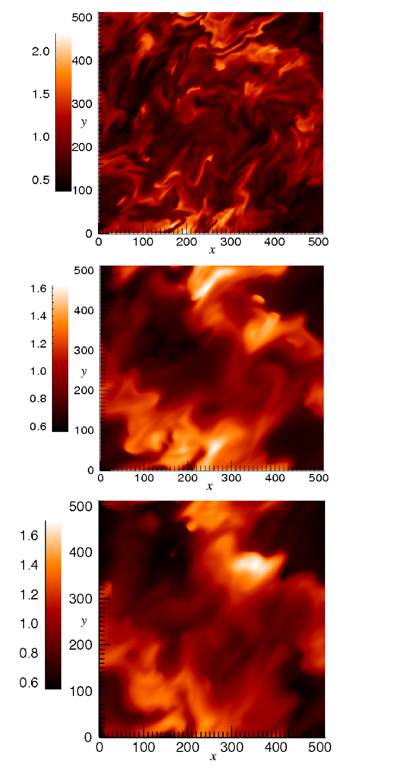
Figure 1: Log plot of the neutral mass density at $t=t_{\rm c}$ in a slice at $z=0.5$ for simulations mhd-512 (upper panel), mc-512 (middle panel) and fr-512 (lower panel).

In figure 2 we present plots of the ambipolar and Hall resistivities for simulation mc-512 for the same times and slices as figure 1. It is clear that the resistivities vary considerably throughout the computational domain with the features strongly correlated with the features in the density distribution. We also show $\eta\equiv\frac{r_{\rm A}}{|r_{\rm H}|}$ to give an indication of the relative importance of each of the resistivities. This, as we shall see, is an important parameter. Finally, figure 3 is the same as 2 except that the data is taken at time $t=0.2t_{\rm c}$ - i.e. after one flow crossing time. Here we can see that the variation of the resistivities in space is dramatic with, for example, the ambipolar resistivity varying by almost 4 orders of magnitude with $\eta$ varying by around 2 orders of magnitude.

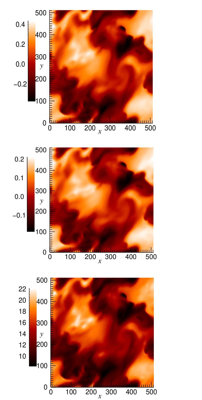
Figure 2: Plot of the normalized ambipolar resistivity (top panel), normalized Hall resistivity (middle panel) and $\eta\equiv\frac{r_{\rm A}}{|r_{\rm H}|}$. Note that the scale is logarithmic in the top and middle panels while it is linear for the bottom panel.

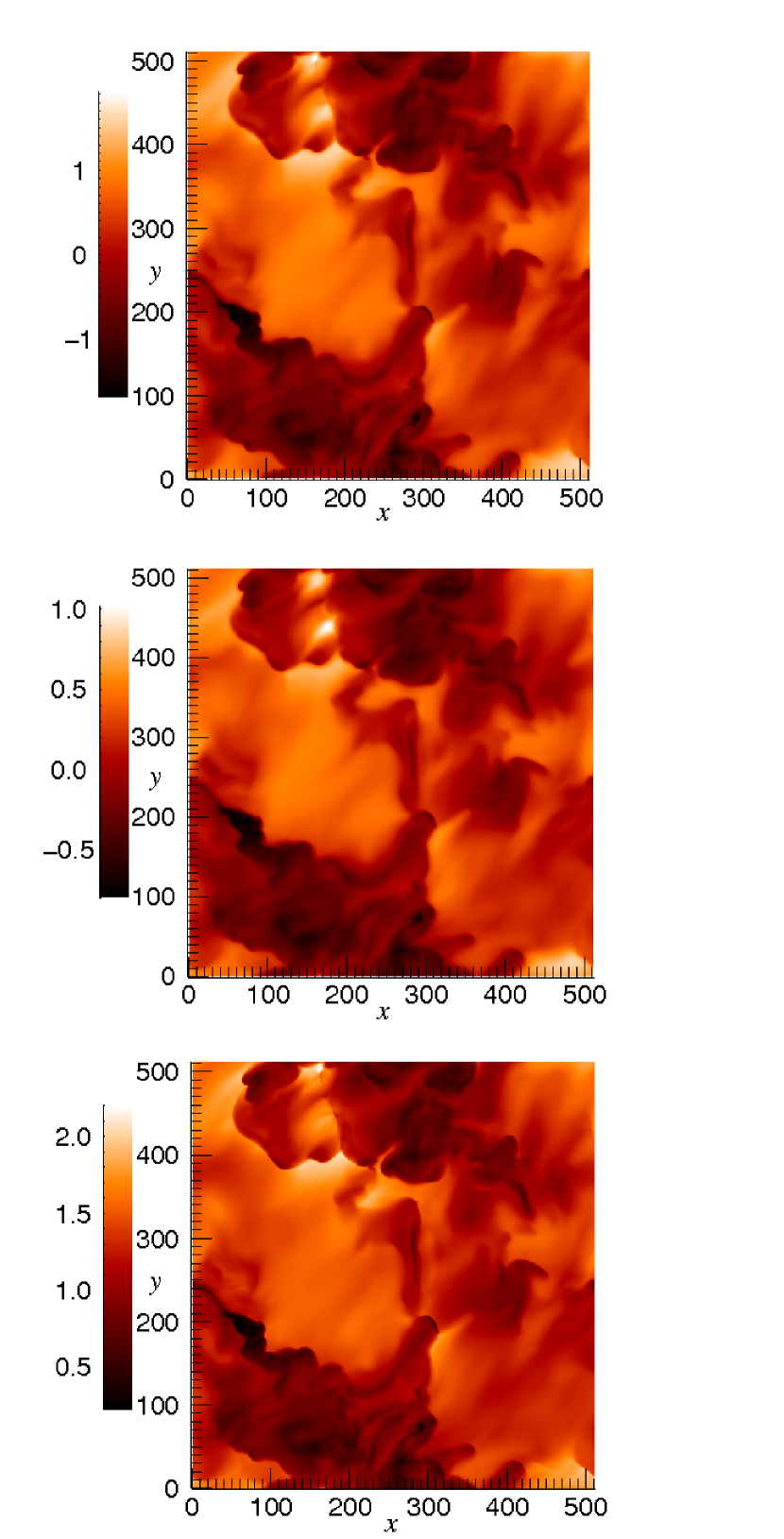
Figure 3: As figure 2 but the snapshots are taken at $t=0.2$ $t_{\rm c}$. Note that the scale here is logarithmic in each case including the bottom panel.

4.1 Resolution study

Four simulations identical in every way except for the resolution were run. Specifically, the resolutions used were $64^{3}$, $128^{3}$, $256^{3}$, and $512^{3}$. We now focus our attention on how the energy decay behaves with resolution. Figure 4 contains plots of the kinetic energy as a function of time for each of the simulations in the resolution study. It is clear that the lower the resolution, the faster the decay - this is what one would expect since lower resolution results in a higher numerical viscosity and hence one expects faster dissipation of energy.

Figure 4: Log scale plot of the kinetic energy (normalized to its initial value) for each of the simulations in the resolution study.

Simulations mc-256 and mc-512 are, however, quite similar in terms of the energy decay with a maximum relative difference of around 10% between the kinetic energies in the simulations at any one time - an almost identical result to that obtained from the resolution study in Paper I. This is notable since in Paper I the resistivities were kept constant in space and time whereas here the resistivities locally increase significantly during the course of the simulations. A reasonable inference is that the influence of local variations in resistivities averages out in some sense on the global scale.

As we shall see later, however, the effect of spatially varying resistivities is noticeable in properties such as the power spectrum of the density and magnetic field.

The various energy decay rates can be modeled approximately as power-laws in time, i.e. $t^{-\beta}$. Fitting the kinetic energy, $\beta_{\rm K}$, magnetic energy, $\beta_{\rm B}$, and total energy, $\beta_{\rm Tot}$, as functions of time in this way we obtain the values given in table 2. This data confirms quantitatively what can be observed in Figure 5 and extends it to the decay of the energy in magnetic perturbations: increasing resolution decreases the rate of energy decay, but the difference between the $256^{3}$ and $512^{3}$ simulations is relatively minor. We note in passing that the decay in the energy in magnetic perturbations is considerably more sensitive to resolution than kinetic energy: $\beta_{\rm B}$ varies between 1.43 and 1.28 while $\beta_{\rm K}$ only varies between 1.38 and 1.34. We know that the resistivities are a critical factor in determining the decay of the magnetic energy since they facilitate loss of magnetic energy through reconnection. We attribute the extra sensitivity to resolution of $\beta_{\rm B}$ to the necessity to properly resolve the diffusive effects in the induction equation, including the variation of the resistivities themselves. The variation of the resistivities throughout the computational domain is significant (see figure 2) and it is interesting to note that $\beta_{\rm B}$ in simulations with fixed resistivities is not so sensitive to resolution (see Paper I).

Table 2: The values of the exponent for the kinetic, magnetic and total energy decay for the simulations presented in this work. These exponents are calculated by fitting the data over the time interval $[0.2t_{\rm c},t_{\rm c}]$.

Simulation	$\beta_{\rm K}$	$\beta_{\rm B}$	$\beta_{\rm Tot}$
mc-64	1.38	1.43	1.39
mc-128	1.37	1.35	1.36
mc-256	1.35	1.30	1.33
mc-512	1.34	1.28	1.32
hall-512	1.12	1.05	1.09
ambi-512	1.35	1.30	1.33
mhd-512	1.12	1.06	1.10
fr-512	1.30	1.28	1.30

4.2 Energy decay

We now discuss the behavior of the kinetic and magnetic energy in our multifluid simulations and compare with those in Paper I.

4.2.1 Kinetic energy decay

Figure 5 contains plots of the decay of kinetic energy with time for the $512^{3}$ resolution simulations outlined in table 1. Note that the kinetic energy decay in all of the simulations is very similar until around $t\approx 0.02\,t_{\rm c}$. This is because at such early times compressions are only just starting to form and so the non-ideal terms in the induction equation have had almost no effect on the dynamics. The subsequent energy decay of simulations mhd-512 and hall-512 are almost identical to each other. The energy decay of simulations mc-512 and ambi-512 are virtually identical over the full plotted range while the data plotted for fr-512 coincide with the former simulations for times in the range $0.03\,t_{\rm c}\leq t\leq 0.2\,t_{\rm c}$. We have fitted the kinetic energy decay as a power-law in the range $0.2t_{\rm c}\leq t\leq t_{\rm c}$ (i.e. after approximately one initial flow crossing time) and the exponents are given in the first column of table 2.

Figure 5: Log scale plot of the kinetic energy (normalized to its initial value) for each of the $512^{3}$ simulations.

It is clear that the presence of ambipolar diffusion has a significant impact on the behavior of the kinetic energy in the turbulent system. This is a result of the exchange of energy between kinetic and magnetic energies as will be discussed in section 4.2.2.

From figure 5 and table 2 it is evident that the Hall effect has almost no impact on the kinetic energy decay in turbulence in molecular clouds. In order to emphasize any possible impact of the Hall effect we have plotted the time evolution of the ratio of the kinetic energy in each of our simulations to that in mc-5-512 in figure 6 on a linear scale. It is clear even in this figure that the Hall effect has little impact on the evolution of the turbulence. This result is also reproduced if we examine the evolution of the magnetic energy (see section 4.2.2). This supports our conclusion from Paper I in which the simulations were run using fixed resistivities (see also fr-512 in this work).

Figure 6: Plot of the ratio of the kinetic energy in our $512^{3}$ simulations to that in mc-5-512

Also shown in figure 5 is the energy decay for simulation fr-512. Given the wide variation of the resistivities in both space and time (see figures 2 and 3) it is somewhat surprising that the energy decay is so similar to that of mc-512. In fact, the volume average of the ambipolar resistivity at $t=0.5$ $t_{\rm c}$ in mc-512 is approximately 60% higher than that in the fr-512 simulation. It would appear that, while ambipolar diffusion enhances energy loss, the expected spatial and temporal variation of it does not have that much influence.

One possible reason for the small divergence between mc-512 and fr-512 would be if the locations in which the resistivity is high are regions in which the magnetic field, $\mathbf{B}$, is varying weakly. To explore this we define a scalar, $\delta B$, by

$$\delta B\equiv|{\rm grad}(B_{x})|+|{\rm grad}(B_{y})|+|{\rm grad}(B_{z})|$$ (25)

where ${\rm grad}(B_{x})$, for example, is a normalized gradient defined by

$${\rm grad}(B_{x})\equiv\frac{1}{B_{0}}\left(\begin{array}[]{c}\delta_{x}B_{x}\\ \delta_{y}B_{x}\\ \delta_{z}B_{x}\end{array}\right)$$ (26)

where $\delta_{\cdot}$ means centered differencing in the indicated direction without normalizing by the zone spacing and $B_{0}$ is the magnitude of the magnetic field throughout the domain at $t=0$. $\delta B$ is then a dimensionless measure of the variation of $\mathbf{B}$ at any point in space or time: if $\delta B$ is large it means there is a high gradient in one or more of the components of $\mathbf{B}$ and therefore resistivity will have an important influence here. Figure 7 contains snapshots of $\delta B$ and $|\mathbf{B}|$ at $t=0.5$ $t_{\rm c}$. There is rich structure in $\delta B$ which is not apparent in $|\mathbf{B}|$.

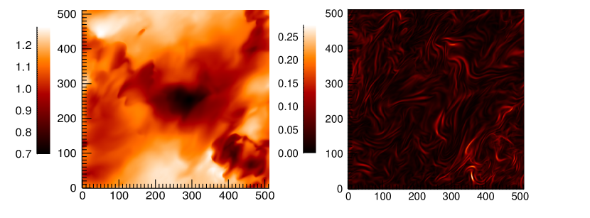
Figure 7: Slices showing the $z=0.5$ plane at $t=0.5$ $t_{\rm c}$ for both $|\mathbf{B}|$ (left panel) and $\delta B$ (right panel).

Figure 8 contains a histogram plot of the two dimensional probability density function for $\delta B$ and $r_{\rm A}$ (the ambipolar resistivity). What is striking about this plot is that there is a notable lack of high $\delta B$ with corresponding high resistivity. Of course, if we have any system in which there are regions of high and low resistivity we expect that, over time, the regions with high diffusion will have lower variation in $\mathbf{B}$ so this, in itself, doesn’t tell us much. However, it does prompt us to look a little more closely at the behavior of $r_{\rm A}$.

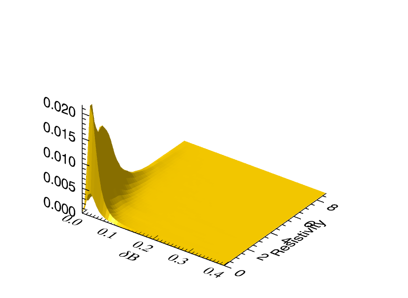
Figure 8: Probability density function for the normalized variation in $\mathbf{B}$ and the resistivity normalized to its initial value (i.e. the same as that used in simulation fr-512). It is clear that high resistivities only occur where there is low variation in $\mathbf{B}$.

Comparison of the middle panel of figure 1 with the top panel of figure 2 shows that the ambipolar resistivity is higher in regions of low density, as would be expected. Now, in supersonic/super-Alfvénic turbulence kinetic energy is dissipated most strongly at strong shocks. However, shocks propagating into regions of very low density will not dissipate kinetic energy effectively. Since it is precisely these regions in which our resistivities are high we must conclude that, in fact, the regions of enhanced resistivity do not contribute significantly to energy dissipation and hence we would not expect the introduction of spatially varying resistivities to increase the rate of energy decay in our simulations. Further, since the volume average of, for example, the ambipolar resistivity is actually higher than that used in fr-512 we would not expect the spatial variation of this resistivity to reduce the rate of energy decay either.

4.2.2 Magnetic energy decay

We now move on to discuss the decay in magnetic energy. Initially, as outlined in Paper I, the magnetic energy increases as the flow compresses and stretches the magnetic field throughout the computational domain. Once this initial increase in the energy has occurred it is gradually lost through two main avenues: magnetic reconnection and transfer of magnetic energy to kinetic energy which can then be dissipated in shocks and other viscous processes.

Figure 9 contains plots of the decay of magnetic energy with time. It is clear that, in common with the case of kinetic energy, the hall-512 and mhd-512 simulations are almost identical while the ambi-512 and mc-512 simulations are also well matched. This supports our inference from section 4.2.1 that the Hall effect has almost no impact on energy decay in molecular clouds on the global scale.

Figure 9: As figure 5 but for magnetic energy.

Ambipolar diffusion does, however, have a significant impact on the behavior of both the kinetic and magnetic energies. This was also noted in Paper I and we explain it in the same way, recapitulated briefly here for completeness. Consider a region of the flow undergoing compression. During this compression kinetic energy will be converted into both magnetic and internal energy through increasing the magnetic pressure and the thermal pressure. Given that this is a turbulent flow we expect that, after some time, this region will begin to expand again. However, during the compression ambipolar diffusion will have diffused away some of the magnetic energy thereby leaving less to be converted back to kinetic energy. In this way the presence of ambipolar diffusion creates a new path through which energy can be lost from the system and reduces the level of all forms of energy in the system.

4.3 Power spectra

We now move on to a study of the power spectra obtained from the multifluid MHD turbulence simulations. These spectra are important from the point of view of understanding the types of structures formed by the turbulence and are a more discerning tool for exploring any structural differences caused by multifluid effects. Table 3 contains the exponents of the power spectra assuming a power-law relationship between power and wave number. All the analysis presented in this section is performed on data taken at $t=t_{\rm c}$.

Table 3: The values of the exponent for the power spectra of density, velocity and magnetic field measured at $t=t_{\rm c}$. All fits are over the range $5\leq k\leq 20$ unless otherwise noted.

Simulation	Density	Velocity	Magnetic field
mc-512	1.82, 4.33	1.34	2.14, 5.38
ambi-512	1.79, 4.31	1.34	2.15, 5.43
hall-512	1.25	1.01	1.51
mhd-512	1.27	1.00	1.55
fr-512	2.11, 4.21	1.28	2.20, 5.53

4.3.1 Density power spectra

We turn first to the scales of the structures formed in the density distributions for our various simulations. Figure 10 contains plots of the power spectra of the neutral density (or density, in the case of simulations mhd-512 and fr-512) for all the $512^{3}$ resolution simulations.

Figure 10: Plot of the normalized, spherically integrated power spectrum of the neutral mass density for each of the $512^{3}$ simulations at $t=t_{\rm c}$.

The power spectra for the simulations including the effects of ambipolar diffusion are approximately broken power laws made up of 3 distinct power laws: $1\,\raisebox{-1.72218pt}{$\stackrel{{\scriptstyle<}}{{\scriptstyle\sim}}$}\,k\,\raisebox{-1.72218pt}{$\stackrel{{\scriptstyle<}}{{\scriptstyle\sim}}$}\,10$, $10\,\raisebox{-1.72218pt}{$\stackrel{{\scriptstyle<}}{{\scriptstyle\sim}}$}\,k\,\raisebox{-1.72218pt}{$\stackrel{{\scriptstyle<}}{{\scriptstyle\sim}}$}\,100$ and $100\,\raisebox{-1.72218pt}{$\stackrel{{\scriptstyle<}}{{\scriptstyle\sim}}$}\,k$. Below the low $k$ break, the spectrum is dependent on the scale of the computational domain. At high $k$ approaching the grid scale, numerical viscosity will begin to dominate. In common with the results presented so far we see that there is little difference between simulations mc-512 and ambi-512 - in fact it is difficult to distinguish between the two spectra without careful examination of figure 10. The fr-512 power spectrum is also similar to mc-512 and ambi-512 although it has slightly less power at intermediate values of $k$ with the difference here being at most 10%.

There is almost no detectable difference between simulations hall-512 and mhd-512. Evidently, the Hall effect has a much weaker influence on the density structure in molecular clouds than ambipolar diffusion. Ambipolar diffusion, on the other hand, has a very significant impact with pronounced damping of density structures at scales less than one tenth of the domain size (corresponding to a physical scale of approximately 0.02 pc). This damping is evident in figure 1 where the density structures in simulations with ambipolar diffusion are more smeared than in mhd-512.

From a quantitative perspective, the data in table 3 shows that the inclusion of ambipolar diffusion significantly steepens the power spectra, increasing the exponent by more than 0.5 over the cases which do not include the effect. The data again suggests that the Hall effect has minimal impact.

The results for fr-512 show a softer spectrum at large length scales and a harder spectrum at short scales than mc-512 and ambi-512, indicating that self-consistent calculation of the resistivities reduces the level of fine structure. This result must, however, be confirmed by higher resolution simulations before it can be regarded as reliable.

Figure 11 contains plots of the power spectra of the neutral density and the density of the negatively charged species at $t=t_{\rm c}$ for comparison. It can be seen that the neutral mass density has more power for $k\geq 10$ although the qualitative shape of the power spectra are the same in each case. This is in qualitative agreement with the results presented in Li et al. (2008) for driven turbulence simulations. For comparison with the results in Table 3, the exponent for the charged species mass density in the range $4\leq k\leq 10$ is -2.21 while in the range $10\leq k\leq 100$ it is -4.84. The power spectrum for the neutral mass density is harder than that for the magnetic field and, in the range $10\leq k\leq 100$, the spectrum for the charged species mass density lies somewhere between the two. This is not surprising as it is a function of the neutral density and velocity (through drag) and the magnetic field (through the Lorentz force).

Figure 11: Plot of the normalized, spherically integrated power spectrum of the neutral and negatively charged mass densities for simulation mc-512.

4.3.2 Velocity power spectra

Figure 12 contains plots of the velocity power spectrum for the neutral velocity. In common with section 4.3.1 those simulations incorporating ambipolar diffusion have significantly less power at almost all scales than those without. This is to be expected given the increased rate of loss of turbulent energy in the presence of ambipolar diffusion (see section 4.2).

Figure 12: Plot of the normalized, spherically integrated power spectrum of the neutral velocity for each of the $512^{3}$ simulations at $t=t_{\rm c}$.

As found in Paper I, and again here, there are clear differences of a qualitative nature between the density power spectra and the velocity power spectra for the multifluid simulations. Those simulations incorporating ambipolar diffusion (mc-512 and ambi-512) exhibit a strong power-law in the range $10\leq k\leq 100$ in the density power spectrum. This is not true of the velocity power spectra. For the latter spectra there is a break at roughly $k\sim 20$ and again at $k\sim 100$. The latter break we interpret as being at the scale where numerical diffusive effects begin to dominate the non-ideal effects in the induction equation. The lower break can reasonably be interpreted as the scale at which the non-ideal effects become important. The marked qualitative differences between the density and velocity power spectra indicate a considerable decoupling between the two variables. It is worth recalling here that the power spectra are calculated at $t=t_{\rm c}$ so it is reasonable to expect that the turbulence is well developed at this stage.

In common with the density power spectra, the presence of ambipolar diffusion produces steeper velocity power spectra (see Table 3) in qualitative agreement with the results of Li et al. (2008).

The results at high $k$ are, of course, dominated by numerical diffusive effects. However, it is interesting to note that simulation fr-512 actually has very slightly less power at short scales than mc-512 despite the volume average of $r_{\rm A}$ being roughly twice as high as the resistivity used in fr-512. This adds weight to the inference from section 4.2.1 that regions of high resistivity tend not to be coincident with regions of high gradients in the magnetic field and therefore do not have the level of influence one would naively expect.

Figure 13 contains plots of the power spectra for the velocity of the neutral and negatively charged species. It can be seen that, except at very high $k$, they are virtually identical. Given that the charged velocity is defined by balance between drag with the neutrals and the Lorentz force this is, perhaps, unsurprising.

Figure 13: Plot of the normalized, spherically integrated power spectrum of the neutral velocity and the velocity of the negatively charged species for simulation mc-512 at $t=t_{\rm c}$.

4.3.3 Magnetic field power spectra

Figure 14 contains plots of the spherically integrated power spectra for the magnetic field. Once again, ambipolar diffusion has a much bigger impact on these spectra than the Hall effect. The magnetic field power spectra are considerably steeper at all $k$ in its presence. The absolute power at any scale is also considerably lowered by ambipolar diffusion, as would be expected from the discussion in section 4.2.2. There is a qualitative similarity between the density power spectra (figure 10) and the magnetic field power spectra which is absent when comparing the latter with the velocity power spectra (see figure 12).

Figure 14: As figure 12 but for the magnetic field.

Interestingly, we see the phenomenon that fr-512 has very slightly less power at $k\geq 20$ than mc-512 indicating that fixing the resistivities at $t=0$ actually results in slightly more dissipation than allowing it to vary in time and space.

We find that the Hall effect has a slightly more noticeable effect on the magnetic field power spectra than on the spectra of velocity or density: it gives rise to a little more structure on short scales which is absent in its absence. This would be expected as the Hall effect is a dispersive effect acting directly on the magnetic field. The results for the density and velocity power spectra, however, demonstrate that this influence over the magnetic power spectra does not translate into an influence over the other variables.

4.4 Velocity dispersion

It has been widely reported that the observed velocity dispersion in molecular clouds behaves as a power-law in the size of the field of view. Figure 15 contains plots of the velocity dispersion for each of the $512^{3}$ resolution simulations presented in this work. As noted in Paper I, and Lemaster & Stone (2009), no power-law is observed. This may be due to the fact that in (multifluid) MHD turbulence there are many relevant signal speeds due to the variation in the orientation and intensity of the magnetic field, in contrast to the situation with hydrodynamic turbulence. Hence there is no reason to expect to see a power-law. Finally, it should be noted that, at this point in the simulation, the turbulence has decayed such that it is largely sub-sonic or transonic. This may also explain the lack of a power-law. Indeed, it should also be noted that our results here are not necessarily in contradiction with observations since the velocity dispersion-size correlation can only be accurately measured in the supersonic regime.

Figure 15: Log-scale plot of the velocity dispersion as a function of length scale for each of the $512^{3}$ simulations. There is no power-law apparent in this data.

It is clear that ambipolar diffusion reduces the velocity dispersion at all length scales - this is what would be expected given the results from the velocity power spectra presented in section 4.3.2. Once again the results here indicate that the Hall effect has little impact. Again, it is interesting to note that the spatial variation of the resistivity in mc-512 appears to have almost no impact as the velocity dispersion seen in fr-512 is almost identical to that in mc-512.

5 Conclusions

We have presented results from a suite of $512^{3}$ resolution simulations of fully multifluid MHD decaying turbulence. The effects incorporated include the Hall effect and ambipolar diffusion. We have performed a resolution study to ensure that the energy decay rate, being the main result presented here, is reliable. We have confirmed the results of the simplified calculations in Paper I that the Hall effect has little impact on the nature and behavior of turbulence in molecular clouds under the well motivated physical parameters assumed in this work. Further, the presence of ambipolar diffusion increases the rate of energy decay at length scales of 0.2 pc and less. The same conclusion is drawn for the behavior of the energy in the magnetic field.

The power spectra for these simulations again suggest that the Hall effect has little impact on the flows with the exception of the spectrum of magnetic field variations. We must keep in mind that the maximum resolution used here ($512^{3}$) is only enough to resolve about half a decade in $k$-space and it is therefore difficult to be confident of the details of the power spectra. Notwithstanding this consideration it does appear clear that ambipolar diffusion steepens the power spectra of the neutral velocity, density and the magnetic field. As noted in Paper I, it appears that at a resolution of $512^{3}$ and an assumed length scale of 0.2 pc we have resolved the length at which ambipolar diffusion begins to influence the turbulent cascade. In Paper I only constant resistivities were implemented and hence it was unclear whether this latter result would survive the inclusion of more realistic fully multifluid MHD in which the resistivities vary strongly in space and time. The results presented here imply that it does.

The power spectra of the neutral velocity and the magnetic field differ qualitatively from that of the density with breaks occurring in the former which are not seen in the latter. This suggests a decoupling between these fields.

The velocity dispersion as a function of length does not behave as a power law. This is not unexpected as the nature of MHD turbulence implies a wide range of applicable signal speeds which can, when combined, remove the power-law behavior which might be expected if only one signal speed were relevant.

References

- Alexiades et al. (1996) Alexiades V., Amiez G., Gremaud P., 1996, Com. Num. Meth. Eng., 12, 31
- Ciolek & Roberge (2002) Ciolek G.E., Roberge, W.G., 2002, ApJ, 567, 947
- Dedner et al. (2002) Dedner, A., Kemm, F., Kröner, D., Munz, C.-D., Schnitzer, T., Wesenberg, M. 2002, J. Comp. Phys., 175, 645
- Downes & O’Sullivan (2008) Downes, T.P., O’Sullivan, S. 2008, Numerical Modeling of Space Plasma Flows: Astronum 2007 ASP Conference Series, N.V. Pogorelov, E. Audit, and G.P. Zank, 385, 12
- Downes & O’Sullivan (2009) Downes, T.P., O’Sullivan, S. 2009, ApJ, Accepted.
- Elmegreen (1993) Elmegreen, B.G. 1993, ApJ, 419, L29
- Elmegreen & Scalo (2004) Elmegreen, B.G., Scalo, J. 2004, ARA&A, 42, 211
- Falle (2003) Falle, S.A.E.G. 2003, MNRAS, 344, 1210
- Glover & Mac Low (2007) Glover, S.C.O., Mac Low, M-M. 2007, ApJ, 659, 131
- Gustaffson et al. (2006) Gustaffson, M., Brandenburg, A., Lemaire, J.L., Field, D., 2006, A&A, 454, 515
- Klein et al. (2003) Klein, R.I., Fisher, R.T., Krumholtz, M.R., McKee, C.F. 2003, Winds, Bubbles and Explosions: A conference to honour John Dyson, S.J. Arthur, W.J. Henney, Rev. Mex. Astron. Astrophys., 15, 92
- Kudoh & Basu (2008) Kudoh, T., Basu, S. 2008, ApJ, 679, L97
- Larson (1981) Larson, R.B. 1981, MNRAS, 194, 809
- Lemaster & Stone (2008) Lemaster, M.N., Stone, J.M. 2008, ApJ, 682, L97
- Lemaster & Stone (2009) Lemaster, M.N., Stone, J.M. 2009, ApJ, 691, 1092
- Li et al. (2008) Li, P.S., McKee, C.F., Klein, R.I., Fisher, R.T. 2008, ApJ, 684, 380
- Mac Low (1999) Mac Low, M.-M. 1999, ApJ, 524, 169
- Mac Low & Klessen (2004) Mac Low, M.-M., Klessen, R.S. 2004, Rev. Mod. Phys., 76, 125
- Mac Low & Ossenkopf (2000) Mac Low, M.-M., Ossenkopf, V. 2000, 353, 339
- Mac Low et al. (1998) Mac Low, M.-M., Klessen, R.S., Burkert, A., Smith, M.D. 1998 Phys. Rev. Lett., 80, 2754
- Matthaeus et al. (2003) Matthaeus, W.H., Dmitruk, P., Smith, D., Ghosh, S., Oughton, S., 2003, Geophys. Res. Lett. 30(21), 2104
- Mininni et al. (2006) Mininni, P.D., Alexakis, A., Pouquet, A. 2006, Journal of Plasma Physics, 73, 377
- Oishi & Mac Low (2006) Oishi, J.S., Mac Low, M.-M. 2006, ApJ, 638, 281
- Ostriker et al. (2001) Ostriker, E.C., Stone, J.M., Gammie, C.F. 2001, ApJ, 546, 980
- O’Sullivan & Downes (2006) O’Sullivan, S., Downes, T.P. 2006, MNRAS, 366, 1329
- O’Sullivan & Downes (2007) O’Sullivan, S., Downes, T.P. 2007, MNRAS, 376, 1648
- Servidio et al. (2007) Servidio, S., Carbone, V., Primavera, L., Veltri, P., Stasiewicz, K. 2007, P&SS, 55, 2239
- Vestuto et al. (2003) Vestuto, J.G., Ostriker, E.C., Stone, J.M. 2003, ApJ, 590, 858
- Wardle (2004) Wardle, M. 2004, Ap&SS, 292, 317
- Wardle & Ng (1999) Wardle, M., Ng, C. 1999, MNRAS, 303, 239