Brauer algebras of type C

Abstract

For each $n\geq 2$, we define an algebra satisfying many properties that one might expect to hold for a Brauer algebra of type ${\rm C}_{n}$. The monomials of this algebra correspond to scalar multiples of symmetric Brauer diagrams on $2n$ strands. The algebra is shown to be free of rank the number of such diagrams and cellular, in the sense of Graham and Lehrer.

keywords: associative algebra, Birman–Murakami–Wenzl algebra, BMW algebra, Brauer algebra, cellular algebra, Coxeter group, Temperley–Lieb algebra, root system, semisimple algebra, word problem in semigroups

AMS 2000 Mathematics Subject Classification: 16K20, 17Bxx, 20F05, 20F36, 20M05

Corresponding author: Arjeh M. Cohen, Department of Mathematics and Computer Science, Eindhoven University of Technology, POBox 513, 5600 MB Eindhoven, The Netherlands, email: A.M.Cohen@tue.nl

1 Introduction

It is well known that the Coxeter group of type ${\rm C}_{n}$ arises from the Coxeter group of type ${\rm A}_{2n-1}$ as the subgroup of all elements fixed by a Coxeter diagram automorphism. Crisp [6] showed that the Artin group of type ${\rm C}_{n}$ arises in a similar fashion from the Artin group of type ${\rm A}_{2n-1}$. In this paper, we study the subalgebra of the Brauer algebra ${\rm Br}({\rm A}_{2n-1})$ of type ${\rm A}_{2n-1}$ (that is, the classical Brauer algebra on $2n$ strands) spanned by Brauer diagrams that are fixed by the symmetry corresponding to this diagram automorphism (see Definition 2.2). Such diagrams will be called symmetric. First, in Definition 2.1, we define the Brauer algebra of type ${\rm C}_{n}$, notation ${\rm Br}({\rm C}_{n})$, in terms of generators and relations depending solely on the Dynkin diagram below.

$${\rm C}_{n}\quad=\quad\mathrel{\mathop{\kern 0.0pt\circ}\limits_{\hbox to0.0pt{\hss$\scriptstyle n-1$\hss}}^{\hbox to0.0pt{\hss$$\hss}}}\kern-1.0pt\vrule height=2.4pt,depth=-2.0pt,width=36.135pt\kern-1.0pt\mathrel{\mathop{\kern 0.0pt\circ}\limits_{\hbox to0.0pt{\hss$\scriptstyle{n-2}$\hss}}^{\hbox to0.0pt{\hss$$\hss}}}\cdots\cdots\mathrel{\mathop{\kern 0.0pt\circ}\limits_{\hbox to0.0pt{\hss$\scriptstyle 2$\hss}}^{\hbox to0.0pt{\hss$$\hss}}}\kern-1.0pt\vrule height=2.4pt,depth=-2.0pt,width=36.135pt\kern-1.0pt\mathrel{\mathop{\kern 0.0pt\circ}\limits_{\hbox to0.0pt{\hss$\scriptstyle 1$\hss}}^{\hbox to0.0pt{\hss$$\hss}}}\kern-4.0pt{{\vrule height=2.0pt,depth=-1.6pt,width=36.135pt}\hbox to0.0pt{\hss\vrule height=4.0pt,depth=-3.6pt,width=36.135pt}\kern-25.0pt<}\kern 8.0pt\mathrel{\mathop{\kern 0.0pt\circ}\limits_{\hbox to0.0pt{\hss$\scriptstyle 0$\hss}}^{\hbox to0.0pt{\hss$$\hss}}}\kern-1.0pt$$

The distinguished generators of ${\rm Br}({\rm C}_{n})$ are the involutions $r_{0},\ldots,r_{n-1}$ and the quasi-idempotents $e_{0},\ldots,e_{n-1}$ (here, a quasi-idempotent is an element that is an idempotent up to a scalar multiple). Each defining relation concerns at most two indices, say $i$ and $j$, and is determined by the diagram induced by ${\rm C}_{n}$ on $\{i,j\}$. The group algebra of the Coxeter group of type ${\rm C}_{n}$ is obtained by taking the quotient of the Brauer algebra of type ${\rm C}_{n}$ by the ideal generated by all quasi-idempotents $e_{i}$. It is isomorphic to the subalgebra generated by all $r_{i}$. The subalgebra generated by all $e_{i}$ $(i=0,\ldots,n-1)$ is isomorphic to the Temperley–Lieb algebra of type ${\rm B}_{n}$ defined by tom Dieck in [7].

The main result states that the algebra ${\rm Br}({\rm C}_{n})$ is isomorphic to the subalgebra ${\rm SBr}({\rm A}_{2n-1})$ of the Brauer algebra ${\rm Br}({\rm A}_{2n-1})$ linearly spanned by symmetric diagrams. In order to distinguish them from those of ${\rm Br}({\rm C}_{n})$, the canonical generators of the Brauer algebra of type ${\rm A}_{2n-1}$ are denoted by $R_{1},\ldots,R_{2n-1}$, $E_{1},\ldots,E_{2n-1}$ instead of the usual lower case letters (see Definition 2.2). Although our formal set-up is slightly more general, the algebras considered are mostly defined over the integral group ring $\mathbb{Z}[\delta^{\pm 1}]$.

Theorem 1.1.

There exists a $\mathbb{Z}[\delta^{\pm 1}]$-algebra isomorphism

$$\phi:{\rm Br}({\rm C}_{n})\longrightarrow{\rm SBr}({\rm A}_{2n-1})$$

determined by $\phi(r_{0})=R_{n}$, $\phi(r_{i})=R_{n-i}R_{n+i}$, $\phi(e_{0})=E_{n}$, and $\phi(e_{i})=E_{n-i}E_{n+i}$, for $0<i<n$. In particular, the algebra ${\rm Br}({\rm C}_{n})$ is free over $\mathbb{Z}[\delta^{\pm 1}]$ of rank $a_{2n}$, where $a_{n}$ is defined by $a_{0}=a_{1}=1$ and, for $n>1$, the recursion

$$a_{n}=a_{n-1}+2(n-1)a_{n-2}.$$

A closed formula for the rank of ${\rm Br}({\rm C}_{n})$ is

$$a_{2n} = \sum_{i=0}^{n}\left(\sum_{p+2q=i}\frac{n!}{p!q!(n-i)!}\right)^{2}\,2^{n-i}\,(n-i)!.$$ (1.1)

A table of $a_{n}$ for some small $n$ is provided below.

$n$	0	1	2	3	4	5	6	7	8
$a_{n}$	1	1	3	7	25	81	331	1303	5937

The paper is structured as follows. In Section 2, we review the definition of a Brauer monoid of any simply laced Coxeter type and introduce the notion of a Brauer algebra of type ${\rm C}_{n}$, denoted ${\rm Br}({\rm C}_{n})$. Section 3 reviews facts about the classical Brauer algebra, denoted ${\rm Br}({\rm A}_{n})$, and about admissible root sets as presented in [4]. These sets lead towards a normal form of monomials closely related to cellularity. In Section 4, we derive elementary properties of ${\rm Br}({\rm C}_{n})$. Next, in Section 5, we prove that the image of $\phi$ is precisely the symmetric diagram subalgebra ${\rm SBr}({\rm A}_{2n-1})$ of ${\rm Br}({\rm A}_{2n-1})$. In Section 6 we study symmetric diagrams, the related algebra ${\rm SBr}({\rm A}_{2n-1})$, and the action of the monoid of all monomials of ${\rm Br}({\rm C}_{n})$ on certain orthogonal root sets and a normal form for monomials in ${\rm Br}({\rm C}_{n})$. With these results, we are able to prove Theorem 1.1 in Section 6. Finally, in Section 7, we establish cellularity (in the sense of [10]) of the newly introduced Brauer algebras and derive some further properties.

We finish this introduction by illustrating our results with the first interesting case: $n=2$. Consider the classical Brauer algebra ${\rm Br}({\rm A}_{3})$. The corresponding Brauer diagrams consist of four nodes at the top and four at the bottom together with a complete matching between these eight nodes. See Figure 1 for interpretations of $R_{i}$ and $E_{i}$ $(i=1,2,3)$. A Brauer diagram is called symmetric if the complete matching is not altered by the reflection of the plane whose mirror is the vertical central axis of the diagram. Clearly, $e_{1}:=E_{1}E_{3}$, $e_{0}:=E_{2}$, $r_{1}:=R_{1}R_{3}$, and $r_{0}:=R_{2}$ represent symmetric diagrams. Our main theorem implies that the subalgebra of ${\rm Br}({\rm A}_{3})$ generated by these diagrams has a presentation on these four generators by the relations given in Definition 2.1 for $n=2$, and moreover it coincides with ${\rm SBr}({\rm A}_{3})$, the linear span of all symmetric diagrams. In fact, it is free and spanned by the following 25 monomials.

$$1,r_{0},r_{1},r_{0}r_{1},r_{1}r_{0},r_{1}r_{0}r_{1},r_{0}r_{1}r_{0}r_{1},r_{0}r_{1}r_{0},$$

$$\{1,r_{1}\}e_{0}\{1,r_{1}r_{0}r_{1}\}\{1,r_{1}\},$$

$$\{1,r_{0},e_{0}\}e_{1}\{1,r_{0},e_{0}\}.$$

The first eight, given on the top line, span a subalgebra isomorphic to the group algebra of the Weyl group of type ${\rm C}_{2}$. This is in accordance with the construction of ${\rm SBr}({\rm A}_{3})$ and the fact that the Weyl group of type ${\rm C}_{2}$ occurs in the Weyl group of type ${\rm A}_{3}$ as the subgroup of elements fixed by a Coxeter diagram automorphism. The two-sided ideal of ${\rm SBr}({\rm A}_{3})$ generated by $e_{1}$ is spanned by the $9$ monomials on the bottom line. Also, the complement in the ideal generated by $e_{0}$ and $e_{1}$ of the ideal generated by $e_{1}$ is spanned by the $8$ monomials on the middle line. This division of the 25 spanning monomials into three parts along the above lines is strongly related to the cellular structure of ${\rm SBr}({\rm A}_{3})$. The subalgebra of ${\rm SBr}({\rm A}_{3})$ generated by $e_{0}$ and $e_{1}$ has dimension 6 and is isomorphic to the Temperley–Lieb algebra of type ${\rm B}_{2}$ introduced by tom Dieck [7]. For these (and other) reasons, we name ${\rm SBr}({\rm A}_{3})$ the Brauer algebra of type ${\rm C}_{2}$. Remarkably, the Temperley–Lieb algebra of type ${\rm B}_{2}$ defined by Graham [9] is 7-dimensional and tom Dieck’s version is a quotient algebra thereof, but we have not found a natural extension of Graham’s algebra to an object deserving the name Brauer algebra of type ${\rm C}_{2}$.

2 Definitions

In this section, we give precise definitions of the algebras and the homomorphism $\phi$ appearing in Theorem 1.1. All rings and algebras given are unital and associative.

Definition 2.1.

Let $R$ be a commutative ring with invertible element $\delta$. For $n\in\mathbb{N}$, the Brauer algebra of type ${\rm C}_{n}$ over $R$ with loop parameter $\delta$, denoted by ${\rm Br}({\rm C}_{n},R,\delta)$, is the $R$-algebra generated by $r_{0}$, $r_{1},\dots,r_{n-1}$ and $e_{0}$, $e_{1},\dots,e_{n-1}$ subject to the following relations.

$$r_{i}^{2} = 1\qquad\qquad\,\,\,\kern 0.20004pt\mbox{for}\,\mbox{any}\ i$$ (2.1)

$$r_{i}e_{i} = e_{i}r_{i}\,=\,e_{i}\,\,\,\,\,\,\kern 0.50003pt\mbox{for}\,\mbox{any}\ i$$ (2.2)

$$e_{i}^{2} = \delta^{2}e_{i}\qquad\quad\,\,\kern 0.20004pt\mbox{for}\ i>0$$ (2.3)

$$e_{0}^{2} = \delta e_{0}$$ (2.4)

$$r_{i}r_{j} = r_{j}r_{i},\qquad\quad\mbox{for}\ i\nsim j$$ (2.5)

$$e_{i}r_{j} = r_{j}e_{i},\qquad\quad\kern-0.29999pt\mbox{for}\ i\nsim j$$ (2.6)

$$e_{i}e_{j} = e_{j}e_{i},\qquad\quad\kern-0.59998pt\mbox{for}\ i\nsim j$$ (2.7)

$$r_{i}r_{j}r_{i} = r_{j}r_{i}r_{j},\qquad\,\kern-0.39993pt\mbox{for}\ {i\sim j}\,\mbox{with}\ i,j>0$$ (2.8)

$$r_{j}r_{i}e_{j} = e_{i}e_{j},\quad\qquad\kern-1.1pt\mbox{for}\ i\sim j\ \mbox{with}\ i,j>0$$ (2.9)

$$r_{i}e_{j}r_{i} = r_{j}e_{i}r_{j},\quad\quad\kern 0.59998pt\mbox{for}\ i\sim j\ \mbox{with}\ i,j>0$$ (2.10)

$$r_{1}r_{0}r_{1}r_{0} = r_{0}r_{1}r_{0}r_{1}$$ (2.11)

$$r_{1}r_{0}e_{1} = r_{0}e_{1}$$ (2.12)

$$r_{1}e_{0}r_{1}e_{0} = e_{0}e_{1}e_{0}$$ (2.13)

$$(r_{1}r_{0}r_{1})e_{0} = e_{0}(r_{1}r_{0}r_{1})$$ (2.14)

$$e_{1}r_{0}e_{1} = \delta e_{1}$$ (2.15)

$$e_{1}e_{0}e_{1} = \delta e_{1}$$ (2.16)

$$e_{1}r_{0}r_{1} = e_{1}r_{0}$$ (2.17)

$$e_{1}e_{0}r_{1} = e_{1}e_{0}$$ (2.18)

Here $i\sim j$ means that $i$ and $j$ are adjacent in the Dynkin diagram ${\rm C}_{n}$. If $R=\mathbb{Z}[\delta^{\pm 1}]$ we write ${\rm Br}({\rm C}_{n})$ instead of ${\rm Br}({\rm C}_{n},R,\delta)$ and speak of the Brauer algebra of type ${\rm C}_{n}$. The submonoid of the multiplicative monoid of ${\rm Br}({\rm C}_{n})$ generated by $\delta$, $\delta^{-1}$, $\{r_{i}\}_{i=0}^{n-1}$, and $\{e_{i}\}_{i=0}^{n-1}$ is denoted by ${\rm BrM}({\rm C}_{n})$. It is the monoid of monomials in ${\rm Br}({\rm C}_{n})$ and will be called the Brauer monoid of type ${\rm C}_{n}$.

Observe that, for a distinguished invertible element $\delta$, the ring $R$ can be viewed as a $\mathbb{Z}[\delta^{\pm 1}]$-algebra and that ${\rm Br}({\rm C}_{n},R,\delta)\cong{\rm Br}({\rm C}_{n})\otimes_{\mathbb{Z}[\delta^{\pm 1}]}R$. As a direct consequence of the above definition, the submonoid of ${\rm BrM}({\rm C}_{n})$ generated by $\{r_{i}\mid i=0,\ldots,n-1\}$ is isomorphic to the Weyl group $W({\rm C}_{n})$ of type ${\rm C}_{n}$.

Let us recall from [4] the definition of a Brauer algebra of simply laced Coxeter type $Q$. In order to avoid confusion with the above generators, the symbols of [4] have been capitalized.

Definition 2.2.

Let $R$ be a commutative ring with invertible element $\delta$ and $Q$ be a simply laced Coxeter graph. The Brauer algebra of type $Q$ over $R$ with loop parameter $\delta$, denoted ${\rm Br}(Q,R,\delta)$, is the $R$-algebra generated by $R_{i}$ and $E_{i}$, for each node $i$ of $Q$ subject to the following relations, where $\sim$ denotes adjacency between nodes of $Q$.

$$R_{i}^{2} = 1$$ (2.19)

$$E_{i}^{2} = \delta E_{i}$$ (2.20)

$$R_{i}E_{i} = =E_{i}R_{i}\,=\,E_{i}$$ (2.21)

$$R_{i}R_{j} = R_{j}R_{i},\,\,\mbox{for}\,\it{i\nsim j}$$ (2.22)

$$E_{i}R_{j} = R_{j}E_{i},\,\,\mbox{for}\,\it{i\nsim j}$$ (2.23)

$$E_{i}E_{j} = E_{j}E_{i},\,\,\mbox{for}\,\it{i\nsim j}$$ (2.24)

$$R_{i}R_{j}R_{i} = R_{j}R_{i}R_{j},\,\,\mbox{for}\,\it{i\sim j}$$ (2.25)

$$R_{j}R_{i}E_{j} = E_{i}E_{j},\,\,\mbox{for}\,\it{i\sim j}$$ (2.26)

$$R_{i}E_{j}R_{i} = R_{j}E_{i}R_{j},\,\,\mbox{for}\,\it{i\sim j}$$ (2.27)

As before, we call ${\rm Br}(Q):={\rm Br}(Q,\mathbb{Z}[\delta^{\pm 1}],\delta)$ the Brauer algebra of type $Q$ and denote by ${\rm BrM}(Q)$ the submonoid of the multiplicative monoid of ${\rm Br}(Q)$ generated by $\delta^{-\pm 1}$ and all $R_{i}$ and $E_{i}$.

For any $Q$, the algebra ${\rm Br}(Q)$ is free over $\mathbb{Z}[\delta^{\pm 1}]$. Also, the classical Brauer algebra on $m+1$ strands is obtained when $Q={\rm A}_{m}$.

Remark 2.3.

As a consequence of the above relations, it is straightforward to show that the following relations hold in ${\rm Br}(Q)$ for all nodes $i$, $j$, $k$ with $i\sim j\sim k$ and $i\not\sim k$ (see [4, Lemma 3.1]).

$$E_{i}R_{j}R_{j} = E_{i}E_{j}$$ (2.28)

$$R_{j}E_{i}E_{j} = R_{i}E_{j}$$ (2.29)

$$E_{i}R_{j}E_{i} = E_{i}$$ (2.30)

$$E_{j}E_{i}R_{j} = E_{j}R_{i}$$ (2.31)

$$E_{i}E_{j}E_{i} = E_{i}$$ (2.32)

$$E_{j}E_{i}R_{k}E_{j} = E_{j}R_{i}E_{k}E_{j}$$ (2.33)

$$E_{j}R_{i}R_{k}E_{j} = E_{j}E_{i}E_{k}E_{j}$$ (2.34)

Remark 2.4.

In [2], Brauer gives a diagrammatic description for a basis of the Brauer algebra of type ${\rm A}_{m}$. Each basis element is a diagram with $2m+2$ dots and $m+1$ strands, where each dot is connected by a unique strand to another dot. Here we suppose the $2m+2$ dots have coordinates $(i,0)$ and $(i,1)$ in $\mathbb{R}^{2}$ with $1\leq i\leq m+1$. The multiplication of two diagrams is given by concatenation, where any closed loops formed are replaced by a factor of $\delta$. The generators $R_{i}$ and $E_{i}$ of ${\rm Br}({\rm A}_{m})$ correspond to the diagrams indicated in Figure 1.

Figure 1: Brauer diagrams corresponding to $R_{i}$ and $E_{i}$.

Each Brauer diagram can be written as a product of elements from $\{R_{i},E_{i}\}_{i=1}^{m}$. This statement is illustrated in Figure 2.

Figure 2: A Brauer diagram and a visualization of it as the product $R_{2}R_{5}E_{1}R_{3}R_{6}E_{2}E_{4}VE_{3}E_{5}E_{7}R_{2}E_{4}E_{6}R_{1}E_{3}E_{5}R_{2}E_{4}$, where $V$ can be either the identity or the simple crossing $R_{1}$.

Henceforth, we identify ${\rm BrM}({\rm A}_{m})$ with its diagrammatic version. It makes clear that ${\rm Br}({\rm A}_{m})$ is a free algebra over $\mathbb{Z}[\delta^{\pm 1}]$ of rank $(m+1)!!$, the product of the first $m+1$ odd integers. The monomials of ${\rm BrM}({\rm A}_{m})$ that correspond to diagrams will be referred to as diagrams.

The map $\sigma$ on the graph (or Coxeter type) ${\rm A}_{m}$ given by $\sigma(i)=m+1-i$ is the single nontrivial automorphism of this graph. As the presentation of ${\rm Br}(Q)$ merely depends on the graph $Q$, the map $\sigma$ induces an automorphism of ${\rm Br}({\rm A}_{m})$, which will also be denoted by $\sigma$. This involutory automorphism is determined by its behaviour on the generators:

$$\sigma(R_{i})=R_{m+1-i},\,\,\,\,\sigma(E_{i})=E_{m+1-i}.$$

The automorphism $\sigma$ may be viewed simply as a reflection of the corresponding diagram about its central vertical axis.

Definition 2.5.

Suppose $D_{1}$ and $D_{2}$ are diagrams in ${\rm Br}({\rm A}_{m})$. The diagram $D_{1}$ is symmetric to the diagram $D_{2}$ if $D_{2}$ is the diagram obtained by taking the reflection of $D_{1}$ about its central vertical axis. If $D_{1}=D_{2}$, then we say $D_{1}$ is a symmetric diagram.

Hence a diagram (that is, a monomial in $R_{i}$ and $E_{i}$) of ${\rm Br}({\rm A}_{m})$ is $\sigma$- invariant if and only if it is symmetric about its central vertical axis. A monomial in ${\rm BrM}({\rm A}_{m})$ is fixed by $\sigma$ if and only if it represents a symmetric diagram.

Lemma 2.6.

Let $m=2n-1$, for some $n\in\mathbb{N}$. The number of symmetric diagrams (with respect to $\sigma$) in ${\rm BrM}({\rm A}_{m})$ is equal to $a_{2n}$, where $a_{n}$ satisfies $a_{0}=a_{1}=1$ and the recursion

$$a_{n}=a_{n-1}+2(n-1)a_{n-2}.$$

Proof.

Fix two sets $X$ and $Y$, say, of size $n$ and a permutation $\tau$ of $X\cup Y$ of order 2 interchanging $X$ and $Y$. We define $a_{n}$ as the number of perfect matchings on $X\cup Y$ that are $\tau$-invariant (that is, if $\{a,b\}\subseteq X\cup Y$ belongs to the matching, so does $\{\tau(a),\tau(b)\}$). Identifying $X$ with the set of dots left of the vertical axis of symmetry, $Y$ with the set of dots to the right, and $\tau$ with the permutation induced by $\sigma$, we see that that $a_{2n}$ is the number of symmetric diagrams in ${\rm BrM}({\rm A}_{m})$.

It is obvious that $a_{0}=a_{1}=1$. Fix $a\in X$. The number of perfect $\tau$-invariant matchings containing $\{a,\tau(a)\}$ is equal to $a_{n-1}$.

Suppose that we have a perfect $\tau$-invariant matching of $X\cup Y$ containing $\{a,b\}$ with $b\neq\tau(a)$. Then $\{\tau(a),\tau(b)\}$ is a second pair belonging to the matching. The matching induces $a_{n-2}$ number of perfect $\tau$-invariant matchings on $(X\cup Y)\setminus\{a,b,\tau(a),\tau(b)\}$. As there are $2n-2$ choices of $b$, we find $a_{n}=a_{n-1}+(2n-2)a_{n-2}$. ∎

Corollary 2.7.

The linear span ${\rm SBr}({\rm A}_{2n-1})$ of symmetric diagrams is a $\mathbb{Z}[\delta^{\pm 1}]$-subalgebra of ${\rm Br}({\rm A}_{2n-1})$. It is free over $\mathbb{Z}[\delta^{\pm 1}]$ of rank $a_{2n}$.

Observe that $R_{n}$, $R_{i}R_{2n-i}$, $E_{n}$, and $E_{i}E_{2n-i}$ are fixed under $\sigma$ for all $i\in\{1,\ldots,n\}$. Thus the image of the map $\phi$ of Lemma 2.8 below lies in ${\rm SBr}({\rm A}_{2n-1})$.

Lemma 2.8.

The following map determines a $\mathbb{Z}[\delta^{\pm 1}]$–algebra homomorphism $\phi:{\rm Br}({\rm C}_{n})\to{\rm SBr}({\rm A}_{2n-1})$.

$\phi(r_{0})=R_{n}$,   $\phi(r_{i})=R_{n-i}R_{n+i}$,

$\phi(e_{0})=E_{n}$  and  $\phi(e_{i})=E_{n-i}E_{n+i}$, for $0<i<n$.

Proof.

It suffices to verify that $\phi$ preserves the defining relations given in Definition 2.1. We demonstrate this for some of the relations (2.1)–(2.18), and leave the rest as an exercise for the reader.

For (2.13):

$$\phi(r_{1})\phi(e_{0})\phi(r_{1})\phi(e_{0}) = R_{n-1}(R_{n+1}E_{n}R_{n+1})R_{n-1}E_{n}$$

$$\overset{(\ref{1.1.10})}{=} R_{n-1}R_{n}E_{n+1}(R_{n}R_{n-1}E_{n})$$

$$\overset{(\ref{1.1.9})}{=} R_{n-1}R_{n}E_{n+1}E_{n-1}E_{n}$$

$$\overset{(\ref{1.1.7})+(\ref{1.1.9})}{=} E_{n}E_{n-1}E_{n+1}E_{n}$$

$$= \phi(e_{0})\phi(e_{1})\phi(e_{0}).$$

For (2.14):

$$\phi(r_{1})\phi(r_{0})\phi(r_{1})\phi(e_{0}) = R_{n+1}(R_{n-1}R_{n}R_{n-1})R_{n+1}E_{n}$$

$$\overset{(\ref{1.1.8})}{=} R_{n+1}R_{n}R_{n-1}(R_{n}R_{n+1}E_{n})$$

$$\overset{(\ref{1.1.9})+(\ref{3.1.1})}{=} R_{n+1}R_{n}R_{n-1}E_{n+1}R_{n}R_{n+1}$$

$$\overset{(\ref{1.1.6})}{=} R_{n+1}R_{n}E_{n+1}R_{n-1}R_{n}R_{n+1}$$

$$\overset{(\ref{1.1.9})+(\ref{3.1.1})}{=} E_{n}R_{n+1}R_{n}R_{n-1}R_{n}R_{n+1}$$

$$\overset{(\ref{1.1.8})}{=} E_{n}R_{n+1}R_{n-1}R_{n}R_{n-1}R_{n+1}$$

$$= \phi(e_{0})\phi(r_{1})\phi(r_{0})\phi(r_{1}).$$

For (2.18):

$$\phi(e_{1})\phi(e_{0})\phi(r_{1}) \overset{(\ref{1.1.5})}{=} E_{n-1}(E_{n+1}E_{n}R_{n+1})R_{n-1}\overset{(\ref{3.1.4})}{=}E_{n-1}E_{n+1}R_{n}R_{n-1}$$

$$\overset{(\ref{1.1.7})+(\ref{3.1.1})}{=} E_{n+1}E_{n-1}E_{n}=\phi(e_{1})\phi(e_{0}).$$

∎

At this point, we have explained the algebras and the map $\phi$ occurring in Theorem 1.1. The surjectivity of $\phi$ will be proved in Proposition 5.16 and its injectivity at the end of Section 6.

3 The classical Brauer algebra

Let $m\in\mathbb{N}$. In this section, we describe the root system of the Coxeter group of type ${\rm A}_{m}$, focussing on special collections of mutually orthogonal positive roots called admissible sets. Also, the notion of height for elements of the Brauer monoid ${\rm BrM}({\rm A}_{m})$ is introduced and discussed. A major goal, established in Theorem 3.9, is to exhibit a normal form for elements of the monoid ${\rm BrM}({\rm A}_{m})$ as a product of generators.

Definition 3.1.

Let $m\geq 1$. The root system of the Coxeter group $W({\rm A}_{m})$ of type ${\rm A}_{m}$ is denoted by $\Phi$. It is realized as $\Phi:=\{{\epsilon}_{i}-{\epsilon}_{j}\mid 1\leq i,j\leq m+1,\ i\neq j\}$ in the Euclidean space $\mathbb{R}^{m+1}$, where ${\epsilon}_{i}$ is the $i^{\mathrm{th}}$ standard basis vector. Put $\alpha_{i}:={\epsilon}_{i}-{\epsilon}_{i+1}$. Then $\{\alpha_{i}\}_{i=1}^{m}$ is called the set of simple roots of $\Phi$. Denote by $\Phi^{+}$ the set of positive roots in $\Phi$ with respect to these simple roots; that is, $\Phi^{+}:=\{{\epsilon}_{i}-{\epsilon}_{j}\mid 1\leq i<j\leq m+1\}$.

We have seen that, up to powers of $\delta$, the monomials of ${\rm Br}({\rm A}_{m})$ correspond to Brauer diagrams. In order to work with the tops and bottoms of Brauer diagrams, we introduce the following notion.

Definition 3.2.

Let $\mathcal{A}$ denote the collection of all subsets of $\Phi$ consisting of mutually orthogonal positive roots. Members of $\mathcal{A}$ are called admissible sets.

An admissible set $B$ corresponds to a Brauer diagram top in the following way: for each $\beta\in B$, where $\beta={\epsilon}_{i}-{\epsilon}_{j}$ for some $i,j\in\{1,\ldots,m+1\}$ with $i<j$, draw a horizontal strand in the corresponding Brauer diagram top from the dot $(i,1)$ to the dot $(j,1)$. All horizontal strands on the top are obtained this way, so there are precisely $|B|$ horizontal strands. The top of the Brauer diagram of Figure 2, corresponds to the admissible set $\{\alpha_{1}+\alpha_{2},\alpha_{2}+\alpha_{3}+\alpha_{4}+\alpha_{5},\alpha_{5}+\alpha_{6}+\alpha_{7}\}$.

Similarly, there is an admissible set corresponding to a Brauer diagram bottom. The bottom of the Brauer diagram of Figure 2, corresponds to the admissible set $\{\alpha_{1}+\alpha_{2}+\alpha_{3}+\alpha_{4}+\alpha_{5}+\alpha_{6}+\alpha_{7},\alpha_{2}+\alpha_{3}+\alpha_{4}+\alpha_{5},\alpha_{4}\}$.

For any $\beta\in\Phi^{+}$ and $i\in\{1,\ldots,m\}$, there exists a $w\in W({\rm A}_{m})$ such that $\beta=w\alpha_{i}$. Then $E_{\beta}:=wE_{i}w^{-1}$ is well defined (see [4, Lemma 4.2]). If $\beta,\gamma\in\Phi^{+}$ are mutually orthogonal, then $E_{\beta}$ and $E_{\gamma}$ commute (see [4, Lemma 4.3]). Hence, for $B\in\mathcal{A}$, we can define the product

$$E_{B} = \prod_{\beta\in B}E_{\beta},$$ (3.1)

which is a quasi-idempotent, and the normalized version

$${\hat{E}}_{B} = \delta^{-|B|}E_{B},$$ (3.2)

which is an idempotent element of the Brauer monoid.

There is an action of the Brauer monoid ${\rm BrM}({\rm A}_{m})$ on the collection $\mathcal{A}$. The generators $R_{i}$ $(i=1,\ldots,m)$ act by the natural action of Coxeter group elements on its root sets, where negative roots are negated so as to obtain positive roots, the element $\delta$ acts as the identity, and the action of $E_{i}$ $(i=1,\ldots,m)$ is defined by

$$E_{i}B:=\begin{cases}B&\text{if}\ \alpha_{i}\in B,\\ B\cup\{\alpha_{i}\}&\text{if}\ \alpha_{i}\perp B,\\ R_{\beta}R_{i}B&\text{if}\ \beta\in B\setminus\alpha_{i}^{\perp}.\end{cases}$$ (3.3)

Alternatively, this action can be described as follows for a monomial $a$: complete the top corresponding to $B$ into a Brauer diagram $b$, without increasing the number of horizontal strands in the top. Now $aB$ is the top of the Brauer diagram $ab$. We will make use of this action in order to provide a normal form for elements of ${\rm BrM}({\rm A}_{m})$. In [4, Definition 3.2], it is shown that this action is well defined for any spherical simply laced type.

The action defined above is a left action. Similarly, there is a right action of ${\rm BrM}({\rm A}_{m})$ on $\mathcal{A}$. In order to interpret the right action of $a$ on $B$, the latter should be pictured as the bottom of a Brauer diagram, so that the bottom corresponding to $Ba$ is the bottom of $ba$. Observe that $a\emptyset$ is the top of the Brauer diagram of $a$ (i.e., the collection of top horizontal strands of $a$ and top row of points) and $\emptyset a$ is its bottom (i.e., the collection of bottom horizontal strands of $a$ and bottom row of points).

Recall that the height ${\rm ht}(\beta)$ of a positive root $\beta\in\Phi^{+}$ is $h$ if it is the sum of precisely $h$ simple roots. This definition will be extended to a height function on $\mathcal{A}$ in such a way that ${\rm ht}(\{\beta\})={\rm ht}(\beta)-1$.

Definition 3.3.

The height of an admissible set $B$, notation ${\rm ht}(B)$, is the minimal number of crossings in a completion of the top corresponding to $B$ to a Brauer diagram without increasing the number of horizontal strands at the top.

For example, the height of the top of the Brauer diagram of Figure 2 is equal to 4 and the height of the bottom is equal to 3.

Definition 3.4.

For every element $a\in{\rm BrM}({\rm A}_{m})$, we define the height of $a$, denoted by ${\rm ht}(a)$, as the minimal number of generators $R_{i}$ needed to write $a$ as a product of the generators $R_{1},\ldots,R_{m},E_{1},\ldots,E_{m}$, $\delta$, $\delta^{-1}$.

In terms of Brauer diagrams, the height of $a$ is the minimal number of crossings needed to draw $a$. Consequently, the height of an admissible set $B$ is the minimal height over all possible Brauer diagram completions of $B$.

The Brauer diagram of Figure 2 has height 7 if $V$ is the identity and height 8 if $V=R_{1}$. The lemma below states some useful properties of this height function.

Remark 3.5.

There is a natural anti-involution on ${\rm Br}({\rm A}_{m})$, denoted by $x\mapsto x^{{\rm op}}$, determined by

$$R_{i}\mapsto\ R_{i}\text{ and }E_{i}\mapsto E_{i}.$$

By anti-involution, we mean a $\mathbb{Z}[\delta^{\pm 1}]$-linear anti-automorphism whose square is the identity.

Lemma 3.6.

Let $B,C\in\mathcal{A}$ with $|B|=|C|$. Then there is a unique diagram $a_{B,C}$ of height ${\rm ht}(B)+{\rm ht}(C)$ in ${\rm BrM}({\rm A}_{m})$ such that $a_{B,C}\emptyset=B$ and $\emptyset a_{B,C}=C$. This diagram satisfies $a_{B,C}a_{B,C}^{{\rm op}}=\delta^{|B|}E_{B}$ as well as $a_{B,C}C=B$ and $Ba_{B,C}=C$.

Proof.

The easiest proof to our knowledge is based on diagrams.

There is a unique way to complete a given top and bottom to a Brauer diagram with a minimal number of crossings: connect the first dot at the top from the left that is not the endpoint of a horizontal strand at the top to the first dot at the bottom that is not the endpoint of a horizontal strand at the bottom; proceed similarly with the second, and so on, until the Brauer diagram is complete. If the top corresponds to $B$ and the bottom to $C$, the resulting diagram is the required monomial $a_{B,C}$. ∎

Lemma 3.7.

Suppose $B\in\mathcal{A}$ has height $0$. Then there are $r=m-2|B|$ diagrams of height 1 in the group of invertible elements in ${\hat{E}}_{B}{\rm BrM}({\rm A}_{m}){\hat{E}}_{B}$ forming a Coxeter system of type ${\rm A}_{r}$. (Here, invertibility is meant with respect to the unit ${\hat{E}}_{B}$ of the monoid).

Proof.

As discussed above, a Brauer diagram with top and bottom corresponding to $B$ has $r+1$ free dots at the top and also $r+1$ at the bottom. For a diagram to be an invertible element in ${\hat{E}}_{B}{\rm BrM}({\rm A}_{m}){\hat{E}}_{B}$, the remaining strands need to be vertical, so they belong to the symmetric group on the $r+1$ free dots at the top (or those at the bottom). Now, up to powers of $\delta$, the idempotent ${\hat{E}}_{B}$ is the element in which all $r$ vertical strands do not cross. Selecting diagrams in which the $i^{\mathrm{th}}$ and $(i+1)^{\mathrm{st}}$ vertical strands cross and no others (for $i=1,2,\ldots,r$), we find the required Coxeter system of type ${\rm A}_{r}$. ∎

Definition 3.8.

For $B\in\mathcal{A}$ of height $0$, denote by $K_{B}$ the Coxeter group determined by Lemma 3.7.

In the middle part of the right hand side of Figure 2, next to $V$, the element $e_{3}e_{5}e_{7}=E_{B}$ appears, where $B=\{\alpha_{3},\alpha_{5},\alpha_{7}\}$ has height $0$. Now $K_{B}$ is a Coxeter group of type ${\rm A}_{1}$, generated by $R_{1}{\hat{E}}_{B}$, so the choices for $V$ are consistent with the possibilities for $V{\hat{E}}_{B}={\hat{E}}_{B}V{\hat{E}}_{B}\in K_{B}$.

Theorem 3.9.

Let $i\in\{0,1,\ldots,\lfloor m/2\rfloor\}$ and let $B$ be any admissible set of size $i$ and of height $0$. Then each element $a$ of ${\rm BrM}({\rm A}_{m})$ with $|a\emptyset|=i$ can be written uniquely as

$$\delta^{k}UVW$$

for certain $k\in\mathbb{Z}$, $U$ a diagram in ${\rm BrM}({\rm A}_{m})E_{B}$ with $UB=a\emptyset$, $W$ a diagram in $E_{B}{\rm BrM}({\rm A}_{m})$ with $\emptyset a=BW$, and $V\in K_{B}$ such that

$${\rm ht}(a)={\rm ht}(U)+{\rm ht}(V)+{\rm ht}(W).$$

Proof.

Take $U=a_{a\emptyset,B}$ and $W=a_{\emptyset a,B}^{{\rm op}}$. Then $V=U^{{\rm op}}aW^{{\rm op}}$ has top and bottom equal to $B$ and so belongs to $K_{B}$. By Lemma 3.6 and (3.2),

$$UVW = a_{a\emptyset,B}a_{a\emptyset,B}^{{\rm op}}aa_{\emptyset a,B}a_{\emptyset a,B}^{{\rm op}}=\delta^{4i}{\hat{E}}_{a\emptyset}a{\hat{E}}_{\emptyset a}=\delta^{k}a$$

for $k=4i$. As ${\rm ht}(U)={\rm ht}(a\emptyset)$ and ${\rm ht}(W)={\rm ht}(\emptyset a)$ and ${\rm ht}(V)$ is the length of $V$ with respect to the Coxeter system of Lemma 3.7, this proves that $a$ has a decomposition as stated.

As for uniqueness, suppose $a=UVW$ is a product decomposition as stated. Then $a\emptyset=UVB=UB=U\emptyset$ (as $U=U{\hat{E}}_{B}$) and $\emptyset U=B$, so by Lemma 3.7 and minimality of the height of $U$, we find $U=a_{a\emptyset,B}$. Similarly, $W$ can be shown to be equal to $a_{\emptyset a,B}^{{\rm op}}$. Finally, $V={\hat{E}}_{B}V{\hat{E}}_{B}=\delta^{-4|B|}U^{{\rm op}}UVWW^{{\rm op}}=\delta^{-4|B|}U^{{\rm op}}aW^{{\rm op}}$ is uniquely determined by $a$, $U$, and $W$. ∎

4 Elementary properties of type ${\rm C}$ algebras

In this section we draw some easy consequences from the definition of a Brauer algebra of type ${\rm C}_{n}$. The results are of use in later sections.

Lemma 4.1.

In ${\rm Br}({\rm C}_{n},R,\delta)$, the following equations hold.

$$r_{1}e_{0}e_{1} = e_{0}e_{1}$$ (4.1)

$$e_{0}e_{1}e_{0} = e_{0}r_{1}e_{0}$$ (4.2)

$$e_{1}r_{0}r_{1}e_{0} = e_{1}e_{0}$$ (4.3)

$$r_{0}r_{1}e_{0}r_{1} = r_{1}e_{0}r_{1}r_{0}$$ (4.4)

$$e_{0}r_{1}e_{0}r_{1} = e_{0}e_{1}e_{0}$$ (4.5)

Proof.

By Definition 2.1,

$$r_{1}e_{0}e_{1}\overset{(\ref{0.1.16})}{=}\delta^{-1}r_{1}e_{0}e_{1}e_{0}e_{1}\overset{(\ref{0.1.19})}{=}\delta^{-1}e_{0}e_{1}e_{0}e_{1}\overset{(\ref{0.1.16})}{=}e_{0}e_{1},$$

proving (4.1). Therefore

$$e_{0}e_{1}e_{0}\overset{(\ref{4.1.2})}{=}r_{1}e_{0}e_{1}e_{0}\overset{(\ref{0.1.19})}{=}r_{1}r_{1}e_{0}r_{1}e_{0}\overset{(\ref{0.1.3})}{=}e_{0}r_{1}e_{0}$$

giving (4.2).

It is easy to check that (4.3) follows from (2.17) and (2.2). Also, the identity (4.4) holds as

$$r_{0}r_{1}e_{0}r_{1} \overset{(\ref{0.1.3})}{=} r_{1}(r_{1}r_{0}r_{1}e_{0})r_{1}\overset{(\ref{0.1.20})}{=}r_{1}e_{0}r_{1}r_{0}r_{1}r_{1}\overset{(\ref{0.1.3})}{=}r_{1}e_{0}r_{1}r_{0}.$$

Finally,

$$(e_{0}r_{1}e_{0})r_{1}\overset{(\ref{4.1.1})}{=}e_{0}(e_{1}e_{0}r_{1})\overset{(\ref{0.1.18})}{=}e_{0}e_{1}e_{0},$$

proving (4.5). ∎

As in the case of type ${\rm A}_{m}$ (see Remark 3.5) there is similarly a natural anti-involution on ${\rm Br}({\rm C}_{n})$. This anti-involution is denoted by the superscript ${\rm op}$, so the map is given by $x\mapsto x^{{\rm op}}$.

Proposition 4.2.

The identity map on $\{\delta,r_{i},e_{i}\mid i=0,\ldots,n-1\}$ extends to a unique anti-involution on the Brauer algebra ${\rm Br}({\rm C}_{n},R,\delta)$.

Proof.

It suffices to check the defining relations given in Definition 2.2 still hold under the anti-involution. An easy inspection shows that all relations involved in the definition are invariant under ${\rm op}$, except for (2.9), (2.12), (2.13), (2.17), and (2.18). The relation obtained by applying ${\rm op}$ to (2.9) holds as can be seen by using (2.10) followed by (2.1) together with (2.9). The equality 2.17 is the op-dual of (2.12). Finally, (4.1) and (4.5) state that the ${\rm op}$ duals of (2.18) and (2.13), respectively, hold. ∎

For each $i\in\{1,\ldots,n\}$, we define the following two elements of ${\rm BrM}({\rm C}_{n})$.

$$y_{i} := r_{i-1}r_{i-2}\cdots r_{1}r_{0}r_{1}\cdots r_{i-2}r_{i-1},$$ (4.6)

$$z_{i} := r_{i-1}r_{i-2}\cdots r_{1}e_{0}r_{1}\cdots r_{i-2}r_{i-1}.$$ (4.7)

Proposition 4.3.

Let $n\geq 2$ and $i\in\{2,\ldots,n\}$ and consider elements in ${\rm BrM}({\rm C}_{n})$.

1. $e_{i},r_{i},y_{i}$, and $z_{i}$ commute with each of $r_{j}$ and $e_{j}$ for $0\leq j\leq i-2$.

2. $y_{i}$ and $z_{i}$ commute with $y_{j}$ and $z_{j}$ for each $j\in\{1,\ldots,n\}$.

Proof.

(i). By Definition 2.1, both $e_{i}$ and $r_{i}$ commute with each element of $\{r_{0},\ldots,r_{i-2},e_{0},\ldots,e_{i-2}\}$.

In order to prove that $y_{i}$ commutes with the indicated elements, we first establish the claim that $y_{i+2}$ commutes with $r_{i}$ and $e_{i}$, for $0\leq i\leq n-2$.

If $i=0$, the claim follows from (2.11) and (2.14), respectively. If $i>0$, we have

$$y_{i+2}r_{i} = r_{i+1}r_{i}\cdots r_{1}r_{0}r_{1}\cdots r_{i}r_{i+1}r_{i}\overset{(\ref{0.1.10})}{=}r_{i+1}r_{i}\cdots r_{1}r_{0}r_{1}\cdots r_{i-1}r_{i+1}r_{i}r_{i+1}$$

$$\overset{(\ref{0.1.7})}{=} r_{i+1}r_{i}r_{i+1}r_{i-1}\cdots r_{1}r_{0}r_{1}\cdots r_{i}r_{i+1}$$

$$\overset{(\ref{0.1.10})}{=} r_{i}r_{i+1}r_{i}\cdots r_{1}r_{0}r_{1}\cdots r_{i-1}r_{i}r_{i+1}=r_{i}y_{i+2},$$

and

$$y_{i+2}e_{i} = r_{i+1}r_{i}\cdots r_{1}r_{0}r_{1}\cdots r_{i}r_{i+1}e_{i}\overset{(\ref{0.1.15})}{=}r_{i+1}r_{i}\cdots r_{1}r_{0}r_{1}\cdots r_{i-1}e_{i+1}r_{i}r_{i+1}$$

$$\overset{(\ref{0.1.8})}{=} r_{i+1}r_{i}e_{i+1}r_{i-1}\cdots r_{1}r_{0}r_{1}\cdots r_{i}r_{i+1}$$

$$\overset{(\ref{0.1.15})}{=} e_{i}r_{i+1}r_{i}\cdots r_{1}r_{0}r_{1}\cdots r_{i-1}r_{i}r_{i+1}=e_{i}y_{i+2}.$$

Now, for arbitrary $i$ and all $0\leq j\leq i-2$, using $y_{i}=r_{i-1}\cdots r_{j+2}y_{j+2}r_{j+2}\cdots r_{i-1}$ and (2.5), we find

$$y_{i}r_{j} = r_{i-1}\cdots r_{j+2}y_{j+2}r_{j+2}\cdots r_{i-1}r_{j}=r_{i-1}\cdots r_{j+2}y_{j+2}r_{j}r_{j+2}\cdots r_{i-1}$$

$$= r_{i-1}\cdots r_{j+2}r_{j}y_{j+2}r_{j+2}\cdots r_{i-1}=r_{j}r_{i-1}\cdots r_{j+2}y_{j+2}r_{j+2}\cdots r_{i-1}$$

$$= r_{j}y_{i}$$

Similarly for $e_{j}$ instead of $r_{j}$, by use of (2.6).

An analogous argument can be used for $z_{i}$. Again, it suffices to show that $z_{i+2}$ commutes with $r_{i}$ and $e_{i}$. For $i=0$ we verify

$$z_{2}e_{0} = (r_{1}e_{0}r_{1})e_{0}\overset{(\ref{0.1.19})+(\ref{4.1.5})}{=}e_{0}(r_{1}e_{0}r_{1})=e_{0}z_{2},$$

$$z_{2}r_{0} = (r_{1}e_{0}r_{1})r_{0}\overset{(\ref{0.1.3})}{=}r_{1}e_{0}r_{1}r_{0}r_{1}r_{1}\overset{(\ref{0.1.20})+(\ref{0.1.3})}{=}r_{0}(r_{1}e_{0}r_{1})=e_{0}z_{2}.$$

For $i>0$, it is straightforward to show that $z_{i+2}r_{i}=r_{i}z_{i+2}$, using (2.5) and (2.8), and $z_{i+2}e_{i}=e_{i}z_{i+2}$, by using a rearrangement of (2.10). Thus, an argument similar to the above proves that $z_{i}r_{j}=r_{j}z_{i}$ and $z_{i}e_{j}=e_{j}z_{i}$, for any $i$ and all $0\leq j\leq i-2$.

As $y_{i}$ and $z_{i}$ are conjugates of $r_{0}$ and $e_{0}$ by the same Coxeter group element, it follows from (2.2) that they commute. It remains to verify that $y_{i}$ and $z_{i}$ commute with $y_{i-1}$ and $z_{i-1}$. But the latter two elements are products of generators from $\{r_{0},\ldots,r_{i-2},e_{0},\ldots,e_{i-2}\}$, which are known to commute with $y_{i}$ and $z_{i}$ by (i) and (ii). This finishes the proof of (i) and (ii). ∎

Remark 4.4.

Using Proposition 4.3, one can prove that for any $n\geq 1$,

$${\rm BrM}({\rm C}_{n})={\rm BrM}({\rm C}_{n-1})\{1,e_{n-1},r_{n-1},y_{n},z_{n}\}{\rm BrM}({\rm C}_{n-1}).$$

This ensures that ${\rm Br}({\rm C}_{n})$ is of finite rank over $\mathbb{Z}[\delta^{\pm 1}]$. Details of the proof of the ensuing ‘normal form’ are surpressed here, as this result is not used in this paper.

5 Surjectivity of $\phi$

The goal of this section is to exhibit a collection of admissible sets on which ${\rm BrM}({\rm C}_{n})$ acts as well as to prove that the map $\phi:{\rm Br}({\rm C}_{n})\longrightarrow{\rm SBr}({\rm A}_{2n-1})$ introduced in Theorem 1.1 is surjective. To this end, we first construct the root system of type ${\rm C}_{n}$ in terms of $\sigma$-fixed vectors in the reflection space for $W({\rm A}_{2n-1})$ spanned by the root system $\Phi$ of Definition 3.1. Notice that the restriction of $\phi$ to the submonoid $W({\rm C}_{n})$ of ${\rm BrM}({\rm C}_{n})$ generated by the $r_{i}$ (isomorphic, as the notation suggests, to the Coxeter group of type ${\rm C}_{n}$) is known to be injective (see, for instance [11]), with image the centralizer of $\sigma$ in the submonoid $W({\rm A}_{2n-1})$ of ${\rm BrM}({\rm A}_{2n-1})$.

We adopt the notation of Section 3 with $m=2n-1$, and will us the root system $\Phi$, the collection of admissible sets $\mathcal{A}$, and the action of ${\rm BrM}({\rm A}_{2n-1})$ on $\mathcal{A}$ defined there. We let the involution $\sigma$ act on the set $\Phi^{+}$ of positive roots of $\Phi$ in the following way, where $\alpha_{i}$ are as in Definition 3.1. For $\Sigma c_{i}\alpha_{i}\in\Phi^{+}$ we decree

$$\sigma(\Sigma c_{i}\alpha_{i})=\Sigma c_{i}\alpha_{2n-i}\qquad(1\leq i<2n).$$

This map $\sigma$ induces the permutation of the simple roots corresponding to the nontrivial automorphism of the Coxeter diagram ${\rm A}_{2n-1}$. This permutation can be extended to the linear transformation of $\mathbb{R}^{2n}$, again denoted $\sigma$, determined by $\sigma({\epsilon}_{i})=-{\epsilon}_{2n+1-i}$. (Indeed, this transformation satisfies $\sigma(\alpha_{i})=\alpha_{2n-i}$ for each $i\in\{1,\ldots,2n-1\}$). The vectors fixed by $\sigma$ form an $n$-dimensional subspace, to be denoted $\mathbb{R}^{2n}_{\sigma}$, of the $(2n-1)$-dimensional subspace of $\mathbb{R}^{2n}$ spanned by $\Phi$.

Definition 5.1.

Let $\mathfrak{p}:\mathbb{R}^{2n}\to\mathbb{R}^{2n}_{\sigma}$ be the orthogonal projection from $\mathbb{R}^{2n}$ onto $\mathbb{R}^{2n}_{\sigma}$, that is, $\mathfrak{p}(x)=(x+\sigma(x))/2$ for $x\in\mathbb{R}^{2n}$. Let $\alpha\in\Phi$. Then $\mathfrak{p}(\alpha)=\alpha$ is of squared norm 2 if $\sigma(\alpha)=\alpha$ and $\mathfrak{p}(\alpha)=\frac{1}{2}(\alpha+\sigma(\alpha))$ is of squared norm $1$ if $\sigma(\alpha)\neq\alpha$. The image $\Psi=\mathfrak{p}(\Phi)$ of $\Phi$ under $\mathfrak{p}$ is a root system of type ${\rm C}_{n}$ with simple roots $\beta_{0}=\mathfrak{p}(\alpha_{n})=\alpha_{n}$ and $\beta_{i}=\mathfrak{p}(\alpha_{n-i})=\mathfrak{p}(\alpha_{n+i})$ for $i=1,\dots,n-1$. It is contained in $\mathbb{R}^{2n}_{\sigma}$ and spans it. Of course, $\Psi^{+}$ will be understood to be the half of $\Psi$ lying in the cone spanned by $\beta_{i}$ $(i=0,\ldots,n-1)$. Given $\alpha\in\Phi$ we write $R_{\alpha}$ for the orthogonal reflection on $\mathbb{R}^{2n}$ with root $\alpha$. Given $\beta\in\Psi$ we write $r_{\beta}$ for the orthogonal reflection on $\mathbb{R}^{2n}_{\sigma}$ with root $\beta$. We may identify $R_{i}$ and $r_{j}$ with $R_{\alpha_{i}}$ and $r_{\beta_{j}}$, respectively.

Recall that $\phi(r_{0})=R_{n}$ and $\phi(r_{j})=R_{n-j}R_{n+j}$ for $j\in\{1,\ldots,n-1\}$.

Lemma 5.2.

The map $\sigma:\mathbb{R}^{2n}\to\mathbb{R}^{2n}$ and the restriction of $\phi$ to $W({\rm C}_{n})$ satisfy the following properties for each $w\in W({\rm C}_{n})$.

1. $\sigma\phi(w)=\phi(w)\sigma$.

2. $\phi(w)x=wx$ if $x\in\mathbb{R}^{2n}_{\sigma}$.

Proof.

As $\sigma R_{i}\sigma^{-1}=R_{2n-i}$ for each $i\in\{1,\ldots,2n-1\}$, we know that $\sigma R_{n}\sigma^{-1}=R_{n}$, and $\sigma R_{n+j}R_{n-j}\sigma^{-1}=R_{n-j}R_{n+j}$, so $\sigma$ commutes with $\phi(r_{j})$ for each $j\in\{0,\ldots,n-1\}$. As $r_{0},\ldots,r_{n-1}$ generate $W({\rm C}_{n})$, this implies that $\sigma$ commutes with each $\phi(w)$ for $w\in W({\rm C}_{n})$. Hence (i).

Also for (ii) it suffices to verify the statement for $w$ a simple reflection. Let $x\in\mathbb{R}^{2n}_{\sigma}$. For $j=0$, we have $\phi(r_{0})x=R_{n}x=r_{0}x$ and for $j=1,\ldots,n-1$, as $(x,\alpha_{n-j})=(x,\alpha_{n+j})$,

$$\phi(r_{j})x = R_{n-j}R_{n+j}x=R_{n-j}(x-(x,\alpha_{n+j})\alpha_{n+j})$$

$$= x-(x,\alpha_{n+j})\alpha_{n+j}-(x,\alpha_{n-j})\alpha_{n-j}$$

$$= x-(x,\alpha_{n+j}+\alpha_{n-j})(\alpha_{n+j}+\alpha_{n-j})/2$$

$$= r_{j}x,$$

as required. ∎

The following result is well known and gives the connection between the restriction of $\phi$ to $W({\rm C}_{n})$ and $\mathfrak{p}$.

Lemma 5.3.

The maps $\mathfrak{p}$ and $\phi$ are compatible in the following two ways.

1. $\mathfrak{p}(\phi(w)\alpha)=w\mathfrak{p}(\alpha)$ for each $w\in W({\rm C}_{n})$ and $\alpha\in\Phi$.

2. $\phi(r_{\beta})=\prod_{\alpha\in\mathfrak{p}^{-1}(\beta)}R_{\alpha}$ and $\phi(e_{\beta})=\prod_{\alpha\in\mathfrak{p}^{-1}(\beta)}E_{\alpha}$ for each $\beta\in\Psi$. Here, the set $\mathfrak{p}^{-1}(\beta)$ has cardinality 1 or 2, according to $\beta\in W({\rm C}_{n})\beta_{0}$ or $\beta\in W({\rm C}_{n})\beta_{1}$.

Proof.

By the definition of $\mathfrak{p}$ and Lemma 5.2,

$$\mathfrak{p}(\phi(w)\alpha) = (\phi(w)\alpha+\sigma(\phi(w)\alpha))/2=(\phi(w)\alpha+\phi(w)\sigma(\alpha))/2$$

$$= \phi(w)(\alpha+\sigma(\alpha))/2=\phi(w)(\mathfrak{p}(\alpha))$$

$$= w(\mathfrak{p}(\alpha)),$$

which proves (i).

As for (ii), let $\beta\in\Psi$. The proofs for $r_{\beta}$ and $e_{\beta}$ are almost identical, so we only give the former. If $\beta$ is simple, the equality $\phi(r_{\beta})=\prod_{\alpha\in\mathfrak{p}^{-1}(\beta)}R_{\alpha}$ holds by definition of $\phi$. Suppose $\beta=w\beta_{0}$ for some $w\in W({\rm C}_{n})$. Then $\beta=\phi(w)\beta_{0}$ by Lemma 5.2(ii) and so, by (i) of the same lemma,

$$\mathfrak{p}(\beta) = \mathfrak{p}(\phi(w)\beta_{0})=w\mathfrak{p}(\beta_{0})=w\beta_{0}=\beta.$$

Now $\mathfrak{p}^{-1}(\beta)=\{\beta\}$ and

$$\phi(r_{\beta}) = \phi(wr_{0}w^{-1})=\phi(w)\phi(r_{0})\phi(w)^{-1}=\phi(w)R_{n}\phi(w)^{-1}$$

$$= R_{\phi(w)\alpha_{n}}=R_{w\alpha_{n}}=R_{\beta}=\prod_{\alpha\in\mathfrak{p}^{-1}\beta}R_{\alpha}.$$

As $\Psi$ is the union of the two $W({\rm C}_{n})$-orbits with representatives $\beta_{0}$ and $\beta_{1}$, it only remains to consider $\beta=w\beta_{1}$ with $w\in W({\rm C}_{n})$. Take $\alpha\in\mathfrak{p}^{-1}(\beta)$. Then $\mathfrak{p}(\phi(w)\alpha_{n-1})=w\mathfrak{p}(\alpha_{n-1})=w\beta_{1}=\beta=\mathfrak{p}(\alpha)$, so, in view of Lemma 5.2(i), $\mathfrak{p}^{-1}(\beta)=\{\phi(w)\alpha_{n-1},\phi(w)\alpha_{n+1}\}$. We find

$$\phi(r_{\beta}) = \phi(wr_{1}w^{-1})=\phi(w)\phi(r_{1})\phi(w)^{-1}=\phi(w)R_{n-1}R_{n+1}\phi(w)^{-1}$$

$$= R_{\phi(w)\alpha_{n-1}}R_{\phi(w)\alpha_{n+1}}=\prod_{\alpha\in\mathfrak{p}^{-1}(\beta)}R_{\alpha},$$

which establishes (ii). ∎

We next consider particular sets of mutually orthogonal positive roots in $\Psi$, and relate them to symmetric admissible sets in $\mathcal{A}$.

Definition 5.4.

Denote by $\mathcal{B}^{\prime}$ the collection of all sets of mutually orthogonal roots in $\Psi^{+}$ and by $\mathcal{A}_{\sigma}$ the subset of $\sigma$-invariant elements of $\mathcal{A}$. As $\mathfrak{p}$ sends positive roots of $\Phi$ to positive roots of $\Psi$, it induces a map $\mathfrak{p}:\mathcal{A}_{\sigma}\to\mathcal{B}^{\prime}$ given by $\mathfrak{p}(B)=\left\{\mathfrak{p}(\alpha)\mid\alpha\in B\right\}$ for $B\in\mathcal{A}_{\sigma}$. An element of $\mathcal{B}^{\prime}$ will be called admissible if it lies in the image of $\mathfrak{p}$. The set of all admissible elements of $\mathcal{B}^{\prime}$ will be denoted $\mathcal{B}$.

Remark 5.5.

Not all sets of mutually orthogonal roots in $\Psi^{+}$ are admissible. For instance $Y=\{\beta_{1},\beta_{1}+\beta_{0}\}$ (two mutually orthogonal short roots) belongs to $\mathcal{B}^{\prime}$ (for $n=2$) but not to $\mathcal{B}$. For, if $X\in\mathcal{A}_{\sigma}$ would be such that $\mathfrak{p}(X)=Y$, then $X$ should contain $\alpha_{1}$ and $\alpha_{3}$ as well as $\alpha_{1}+\alpha_{2}$ and $\alpha_{2}+\alpha_{3}$; but these roots are not mutually orthogonal. On the other hand, for $n\geq 4$, the unordered pair $\{\beta_{1},\beta_{3}\}$ from another $W({\rm C}_{n})$-orbit of mutually orthogonal short roots, is the image of the admissible set $\{\alpha_{n-1},\alpha_{n+1},\alpha_{n-3},\alpha_{n+3}\}$ and so belongs to $\mathcal{B}$.

Also $\{\beta_{0},2\beta_{1}+\beta_{0}\}$ (two mutually orthogonal long roots) does belong to $\mathcal{B}$ (for $n=2$) as it coincides with $\mathfrak{p}(X)$, where $X=\{\alpha_{n},\alpha_{n-1}+\alpha_{n}+\alpha_{n+1}\}$.

Proposition 5.6.

The monoid ${\rm BrM}({\rm C}_{n})$ acts on $\mathcal{A}_{\sigma}$ under the composition of the above action and $\phi$.

Proof.

It suffices to prove that $\mathcal{A}_{\sigma}$ is closed under the action of $\phi({\rm BrM}({\rm C}_{n}))$. It is easy to see that $\sigma(a)\sigma(B)=\sigma(aB)$, for $a\in{\rm BrM}({\rm A}_{2n-1})$ and $B\in\mathcal{A}$. Consequently, if $a\in{\rm BrM}({\rm A}_{2n-1})_{\sigma}$ and $B\in\mathcal{A}_{\sigma}$, then it follows that $aB=\sigma(a)\sigma(B)=\sigma(aB)$. This shows $aB\in\mathcal{A}_{\sigma}$. As $\phi({\rm BrM}({\rm C}_{n}))\subseteq{\rm BrM}({\rm A}_{2n-1})_{\sigma}$, the proposition follows. ∎

Proposition 5.7.

The map $\mathfrak{p}:\mathcal{A}_{\sigma}\to\mathcal{B}$ is bijective and $W({\rm C}_{n})$-equivariant, so $\mathfrak{p}(\phi(w)X)=w\mathfrak{p}(X)$ for $X\in\mathcal{A}_{\sigma}$ and $w\in W({\rm C}_{n})$.

Proof.

The map $\mathfrak{p}$ is surjective by definition of $\mathcal{B}$. Let $Y\in\mathcal{B}$ and $X\in\mathfrak{p}^{-1}(Y)$. If $\beta\in Y$, then there is $\alpha\in X$ such that $\beta=\mathfrak{p}(\alpha)$. As $X\in\mathcal{A}_{\sigma}$, it follows that $\sigma\alpha\in X$, so $X=\{\alpha\in\Phi\mid\mathfrak{p}(\alpha)\in Y\}$ is uniquely determined by $Y$. This shows that $\mathfrak{p}$ is injective.

Finally, if in addition, $w\in W({\rm C}_{n})$, then $\phi(w)X\in\mathcal{A}_{\sigma}$ by Proposition 5.6, and, by Lemma 5.3,

$$\mathfrak{p}(\phi(w)X) = \{\mathfrak{p}(\phi(w)\alpha)\mid\alpha\in X\}=w\{\mathfrak{p}(\alpha)\mid\alpha\in X\}=w\mathfrak{p}(X).$$

∎

Lemma 5.8.

Let $i$ and $j$ be nodes of the Dynkin diagram ${\rm C}_{n}$. If $w\in W({\rm C}_{n})$ satisfies $w\beta_{i}=\beta_{j}$, then $we_{i}w^{-1}=e_{j}$.

Proof.

Observe that $w\beta_{i}=\beta_{j}$ only holds for distinct $i$ and $j$ if $i,j>0$, in which case the existence of such a $w$ is a direct consequence of known results on Coxeter groups. The full statement then follows from the fact that all generators of the stabilizer of $\beta_{i}$ in $W({\rm C}_{n})$ also stabilize $e_{i}$, which we prove now.

Suppose $i>0$. As

$$r_{1}e_{1}r_{1} \overset{(\ref{0.1.4})}{=} e_{1},$$

$$r_{0}(r_{1}r_{0}e_{1}r_{0}r_{1})r_{0} \overset{(\ref{0.1.14})+(\ref{0.1.17})}{=} r_{0}r_{0}e_{1}r_{0}r_{0}=e_{1},$$

$$y_{3}e_{1}y_{3} \overset{\ref{X_n}}{=} e_{1}y_{3}y_{3}=e_{1},$$

$$r_{i}e_{1}r_{i} \overset{(\ref{0.1.9})}{=} e_{1}r_{i}r_{i}=e_{1},\,\mbox{for}\,\,i>3,$$

the elements $r_{1}$, $r_{0}r_{1}r_{0}$, $y_{3}$, $r_{3}$,$\ldots$, $r_{n-1}$ stabilize $e_{1}$. But these elements are known to generate the full stabilizer in $W({\rm C}_{n})$ of $\beta_{1}$, so $w\beta_{1}=\beta_{1}$ implies $we_{1}w^{-1}=e_{1}$ for every $w\in W({\rm C}_{n})$.

If one of $i$ and $j$ is $0$, then they both are, as $(we_{i}w^{-1})^{2}=\delta^{k}we_{i}w^{-1}$, where $k=2$ if $i>0$ and $k=1$ otherwise (see (2.3) and (2.4)).

It is known that the stabilizer of $\beta_{0}$ is generated by $r_{0}$, $r_{1}r_{0}r_{1}$, and $r_{i}$ $(i=2,\dots,n-1)$. These elements also centralize $e_{0}$:

$$r_{0}e_{0}r_{0} \overset{(\ref{0.1.4})}{=} e_{0},$$

$$r_{1}r_{0}r_{1}e_{0}r_{1}r_{0}r_{1} \overset{(\ref{0.1.20})}{=} e_{0},$$

$$r_{i}e_{0}r_{i} \overset{(\ref{0.1.8})}{=} e_{0}\qquad\mbox{for}\,\,i>1.$$

This ends the proof of the lemma. ∎

Consider a positive root $\beta$ and a node $i$ of type ${\rm C}_{n}$. If there exists $w\in W$ such that $w\beta_{i}=\beta$, then we can define the element $e_{\beta}$ in ${\rm BrM}({\rm C}_{n})$ by

$$e_{\beta}=we_{i}w^{-1}.$$

The above lemma implies that $e_{\beta}$ is well defined. In general,

$$we_{\beta}w^{-1}=e_{w\beta},$$

for $w\in W({\rm C}_{n})$ and $\beta$ a root of $W({\rm C}_{n})$. Note that $e_{\beta}=e_{-\beta}$ in view of (2.2).

In this perspective, we can reinterpret the element $y_{i}$ of (4.6) as $r_{\gamma}$ and $z_{i}$ of (4.7) as $e_{\gamma}$, where $\gamma=\beta_{0}+2\beta_{1}+\cdots+2\beta_{i-1}$. Proposition 4.3 shows that, for each $i\in\{0,\ldots,n-1\}$,

$$b_{i} = \prod_{k=1}^{i}z_{k}$$ (5.1)

is well defined. The admissible set

$$B_{i} = \mathfrak{p}^{-1}\left(\{\beta_{0},\beta_{0}+2\beta_{1},\ldots,\beta_{0}+2\beta_{1}+\cdots+2\beta_{i-1}\}\right)$$ (5.2)

in $\mathcal{A}_{\sigma}$ is both the top and the bottom of $\phi(b_{i})$. In other words, the symmetric diagram of $b_{i}$ has horizontal strands from $(n+1-j,1)$ to $(n+j,1)$ and from $(n+1-j,0)$ to $(n+j,0)$ for each $j\in\{1,\ldots,i\}$. This is the special case $p=i$ of the top displayed in Figure 3. Later, below (5.5), we will use this fact. The $B_{i}$ $(i=0,\ldots,n)$ are a complete set of $W({\rm A}_{m})$-orbit representatives in $\mathcal{A}$. Moreover, $\phi(b_{i})$ has height $0$.

Proposition 5.9.

Let $\beta$ and $\gamma$ be positive roots of $\Psi$.

1. $e_{\beta}r_{\beta}=r_{\beta}e_{\beta}=e_{\beta}$, $e_{\beta}^{2}=\delta^{2}e_{\beta}$ if $\beta$ is short, and $e_{\beta}^{2}=\delta e_{\beta}$ if $\beta$ is long.

2. If $(\beta,\gamma)=\pm 1$ and $\beta$ and $\gamma$ are short, then $e_{\beta}r_{\gamma}e_{\beta}=e_{\beta}$, $r_{\beta}r_{\gamma}e_{\beta}=e_{\gamma}r_{\beta}r_{\gamma}=e_{\gamma}e_{\beta}$, and $e_{\beta}e_{\gamma}e_{\beta}=e_{\beta}$.

3. If $(\beta,\gamma)=\pm 1$ with $\beta$ short and $\gamma$ long, then the equations (2.11)–(2.18) and (4.1)–(4.5) still hold with the subscripts $1$ and $0$ replaced by $\beta$ and $\gamma$, respectively.

4. If $(\beta,\gamma)=0$ and $\beta$ and $\gamma$ are both long, then $e_{\beta}e_{\gamma}=e_{\beta}e_{\gamma}$.

5. If $(\beta,\gamma)=0$ and $\beta$ and $\gamma$ are both short, and there exists a long positive root $\alpha$ such that $\beta=\gamma+\alpha$ or $\beta=\gamma-\alpha$, then $e_{\beta}e_{\gamma}=\delta r_{\alpha}e_{\gamma}$ or $e_{\gamma}e_{\beta}=\delta r_{\alpha}e_{\beta}$. In each case, $e_{\beta}e_{\gamma}\neq e_{\gamma}e_{\beta}$.

Proof.

The assertions are easily proved after reduction to simple cases using Lemma 5.8. We illustrate the argument by treating (v) now in greater detail.

Up to an interchange of $\beta$ and $\gamma$, there exists $w\in W({\rm C}_{n})$ such that $w\beta_{0}=\alpha$ and $w\beta_{1}=\gamma$ and $\beta=\gamma+\alpha=r_{\alpha}\gamma$. Now $e_{\beta}e_{\gamma}=r_{\alpha}e_{\gamma}r_{\alpha}e_{\gamma}=wr_{0}e_{1}r_{0}e_{1}w^{-1}\overset{(\ref{0.1.12})}{=}\delta wr_{0}e_{1}w^{-1}=\delta r_{\alpha}e_{\gamma}$. The inequality stated at the end of part (v) follows from the inspection of symmetric Brauer diagrams in the image of $\phi$. ∎

As a consequence of Proposition 5.9(iv) and (2.7), the product of $e_{\beta}$, for $\beta$ running over the members of an admissible set, does not depend on the order. Therefore, for each $B\in\mathcal{B}$, we may define

$$e_{B} = \prod_{\beta\in B}e_{\beta},$$ (5.3)

This is very similar to the definition of $E_{B}$ in (3.2). Part (v) of the proposition shows that it is essential that $B$ be admissible for a set $B$ of orthogonal roots to define a product as in (5.3). There exists another $W({\rm C}_{n})$-orbit of pairs of mutually orthogonal positive roots than those in part (v) of the previous proposition; these lead to admissible sets and behave well in (5.3) in view of (2.7).

As $W({\rm C}_{n})$ is a subgroup of the monoid ${\rm BrM}({\rm C}_{n})$, it also acts on $\mathcal{A}_{n}$ (cf. Proposition 5.6). We will show that the admissible sets defined below are orbit representatives for this action.

Definition 5.10.

For $i$ and $p$ with $0\leq p\leq i\leq n$ and $i-p$ even, write

$$e_{i,p} = e_{p+1}e_{p+3}\cdots e_{i-1},$$ (5.4)

and

$$B_{i,p} = e_{p+1}e_{p+3}\cdots e_{i-1}B_{i}.$$

In addition, for $p^{\prime}\in\mathbb{N}$ with $0\leq p^{\prime}\leq i<n$ and $i-p^{\prime}$ even, we write

$$b_{p,i,p^{\prime}} = e_{i,p}b_{i}e_{i,p^{\prime}},$$ (5.5)

where $b_{i}$ is as defined in (5.1).

Figure 3: The admissible set $B_{i,p}$.

Observe that $B_{i,i}=B_{i}$. The admissible set $B_{i,p}$ is pictured in Figure 3 as the top of a Brauer diagram.

Lemma 5.11.

If $0<p,p^{\prime}<i$ with $i-p$ and $i-p^{\prime}$ even, then $\phi(b_{p,i,p^{\prime}})$ is a diagram of height $0$ with top $B_{i,p}$ and bottom $B_{i,p^{\prime}}$. Moreover, $\phi(b_{p,i,p^{\prime}})=a_{B_{i,p},B_{i,p^{\prime}}}$.

Proof.

This is an easy verification involving the left and right monoid actions of Proposition 5.6 (use that $e_{i,p^{\prime}}^{{\rm op}}=e_{i,p^{\prime}}$). ∎

Recall that the Temperley–Lieb subalgebra of ${\rm Br}({\rm C}_{n})$ is the subalgebra generated by $e_{0},\ldots,e_{n-1}$, and similarly for ${\rm Br}({\rm A}_{m})$ and for the corresponding monoids. The following lemma implies that the restriction of $\phi$ to the Temperley–Lieb subalgebra of ${\rm Br}({\rm C}_{n})$ behaves as required.

Lemma 5.12.

Let $B\in\mathcal{A}_{\sigma}$. Then $E_{B}=\phi(e_{\mathfrak{p}(B)})$ and, in particular, hence $E_{B}\in\phi({\rm Br}({\rm C}_{n}))$. Moreover, the restriction of $\phi$ to the Temperley–Lieb subalgebra of ${\rm Br}({\rm C}_{n})$ is surjective onto the intersection of the Temperley–Lieb algebra of ${\rm Br}({\rm A}_{2n-1})$ with ${\rm SBr}({\rm A}_{2n-1})$.

Proof.

Suppose $B\in\mathcal{A}_{\sigma}$. Then, by Lemmas 5.3(ii) and 2.8,

$$E_{B} = \prod_{\alpha\in B}E_{\alpha}=\prod_{\beta\in\mathfrak{p}(B)}E_{\mathfrak{p}^{-1}(\beta)}=\prod_{\beta\in\mathfrak{p}(B)}\phi(e_{\beta})=\phi\left(\prod_{\beta\in\mathfrak{p}(B)}e_{\beta}\right)=\phi(e_{\mathfrak{p}(B)}),$$

as required for the first statements.

Let $\bar{i}\in\{0,1\}$ be such that $i\equiv\bar{i}\pmod{2}$. Then $B_{i,\bar{i}}$ consists of simple roots only and belongs to the same $W({\rm A}_{2n-1})$-orbit in $\mathcal{A}$ as $B_{i}$ or in fact $B_{i,p}$ for any $p$.

As for the last statement, suppose that $a\in{\rm SBr}({\rm A}_{2n-1})$ is a monomial in the Temperley–Lieb subalgebra of ${\rm Br}({\rm A}_{2n-1})$. Then, up to powers of $\delta$, there are $i\in\{0,\ldots,n\}$ and $B,B^{\prime}\in\mathcal{A}_{\sigma}$ of height $0$ with $a=a_{B,B^{\prime}}=(a_{B,B_{i,\bar{i}}})(a_{B^{\prime},B_{i,\bar{i}}})^{\rm op}$ in the notation of and by use of Lemma 3.6. In view of the opposition involution and the first statement of this proposition, it suffices to show that $a:=a_{B,B_{i,\bar{i}}}$ lies in the image under $\phi$ of the submonoid of ${\rm BrM}({\rm C}_{n})$ generated by $e_{0},e_{1},\ldots,e_{n-1}$, the Temperley–Lieb submonoid of ${\rm BrM}({\rm C}_{n})$. To this end, let $B\in\mathcal{A}_{\sigma}$ be of height $0$. We will establish the existence of an element $b$ in this Temperley–Lieb submonoid with $\phi(b)B_{i,\bar{i}}=B$. This will suffice as then Theorem 3.9 gives $a=E_{B}\phi(b)=\phi(e_{\mathfrak{p}(B)}b)$, up to powers of $\delta$, and so $a\in\phi({\rm BrM}({\rm C}_{n}))$.

For $\gamma_{1}=\epsilon_{i_{1}}-\epsilon_{j_{1}}$ and $\gamma_{2}=\epsilon_{i_{2}}-\epsilon_{j_{2}}\in\Phi^{+}$, we say $\gamma_{1}\ll\gamma_{2}$ if $1\leq i_{2}<i_{1}<j_{1}<j_{2}\leq 2n$. If $\gamma_{1}\ll\gamma_{2}\ll\cdots\ll\gamma_{s}$, and $\gamma_{k}\in B$, for $1\leq k\leq s$, we say that $\gamma_{1}\ll\gamma_{2}\ll\cdots\ll\gamma_{s}$ is a chain in $B$, and call $s$ the length of this chain. Now we use induction on the maximal length $t$ of a chain in $B$ and the number $l$ of longest chains in $B$.

Suppose first $t=1$. Then $B$ consists of simple roots and $b$ as required can be found easily. Suppose $t>1$. Let $\gamma_{1}\ll\gamma_{2}\ll\cdots\ll\gamma_{t}$ be a longest chain of $B$ with $r_{2}=\epsilon_{j_{2}}-\epsilon_{i_{2}}$. Since $a$ is an element of the Temperley–Lieb submonoid of ${\rm BrM}({\rm A}_{2n-1})$, $j_{2}-i_{2}$ is odd, and for $1\leq k\leq r=[(j_{2}-i_{2})/2]$ we have $\epsilon_{i_{2}+2k-1}-\epsilon_{i_{2}+2k}\in B$. Let

$$D = \{\gamma_{2}\}\cup\{\epsilon_{i_{2}+2k-1}-\epsilon_{i_{2}+2k}\}_{k=1}^{r},$$

$$D^{\prime} = \{\epsilon_{i_{2}+2k}-\epsilon_{i_{2}+2k+1}\}_{k=0}^{r},$$

$$B^{\prime} = (B\setminus D\cup\sigma(D))\cup(D^{\prime}\cup\sigma(D^{\prime})).$$

Now $B^{\prime}\in\mathcal{A}_{\sigma}$ is the top of a Temperley–Lieb element with maximal length less than $t$ or number of maximal chains fewer than $l$. By the induction hypothesis there exists some Temperley–Lieb element $b^{\prime}$ in ${\rm BrM}({\rm C}_{n})$ with $\phi(b^{\prime})B_{i}=B^{\prime}$. It satisfies

$$E_{X}(D^{\prime}\cup\sigma(D^{\prime}))=D\cup\sigma(D)\qquad\mbox{ and }\qquad E_{X}(B^{\prime})=B,$$

where $X=(D\setminus\{\gamma_{2}\})\cup\sigma(D\setminus\{\gamma_{2}\})\in\mathcal{A}_{\sigma}$. As $E_{X}=\phi(e_{\mathfrak{p}(X)})$ by the first statement of the lemma, we conclude that $\phi(e_{\mathfrak{p}(X)}b^{\prime})B_{i,\bar{i}}=B$, which proves the lemma. ∎

Definition 5.13.

Let $i\in\{0,\ldots,n\}$. Define ${\hat{E}}^{(i)}$ to be the idempotent in ${\rm BrM}({\rm A}_{2n-1})$ corresponding to $b_{i}$;

$${\hat{E}}^{(i)} := \delta^{-i}\phi(b_{i}).$$

In addition, define

$${\hat{b}}^{(i)} := \delta^{-i}e_{\mathfrak{p}(B_{i})}.$$ (5.6)

Then ${\hat{E}}^{(i)}=\phi({\hat{b}}^{(i)})$ by Lemma 5.12. Furthermore, we write $K_{i}$ instead of $K_{B_{i}}$ as introduced in Definition 3.8.

Observe that $K_{i}$ is generated by

$$\hskip-19.91684pt{\hat{E}}^{(i)}R_{n\pm\lfloor 2+i/2\rfloor},{\hat{E}}^{(i)}R_{n\pm\lfloor 3+i/2\rfloor},\ldots,{\hat{E}}^{(i)}R_{n\pm(n-1)},\mbox{\ and \ }{\hat{E}}^{(i)}R_{0},$$ (5.7)

where $R_{0}$ stands for the longest reflection of $W({\rm A}_{2n-1})$, that is,

$$(R_{1}R_{2n-1})(R_{2}R_{2n-2})\cdots(R_{n-1}R_{n+1})R_{n}(R_{n-1}R_{n+1})\cdots(R_{2}R_{2n-2})(R_{1}R_{2n-1}).$$

The definition of $y_{i}$ from (4.6) shows that $\phi(y_{n})=R_{0}$.

We will now prove that the $\sigma$-fixed part of $K_{i}$ is contained in the image of $\phi$, making use of the fact that $K_{i}$ is a Coxeter group of which the above generators are a Coxeter system, as given by Lemma 3.7.

Lemma 5.14.

Let $i\in\{0,\ldots,n\}$. The set (5.7) of simple reflections of $K_{i}$ is invariant under $\sigma$. In fact, $\sigma$ induces the nontrivial automorphism on the Coxeter type ${\rm A}_{2(n-j)-1}$ of $K_{i}$, where $j=1+\lfloor i/2\rfloor$. As a consequence, the subgroup of $\sigma$-fixed elements of $K_{i}$ is of type ${\rm C}_{n-j}$ and is generated by the images under $\phi$ of ${\hat{b}}^{(i)}r_{j+1},{\hat{b}}^{(i)}r_{j+2},\ldots,{\hat{b}}^{(i)}r_{n-1}$, and ${\hat{b}}^{(i)}y_{n}{\hat{b}}^{(i)}$.

Proof.

Clearly, $\sigma$ fixes ${\hat{E}}^{(i)}=\phi({\hat{b}}^{(i)})$. Moreover, it fixes $R_{0}$ and interchanges $R_{n-k}$ and $R_{n+k}$, so indeed the Coxeter system of $K_{i}$ is $\sigma$-invariant and $\sigma$ induces the nontrivial automorphism on the Coxeter type ${\rm A}_{2(n-j)-1}$ of $K_{i}$. It is well known (cf. [11]) that the subgroup of $\sigma$-fixed elements of $K_{i}$ is generated by the Coxeter system

$${\hat{E}}^{(i)}R_{j+1}R_{2n-j-1},{\hat{E}}^{(i)}R_{j+2}R_{2n-j-2},\ldots,{\hat{E}}^{(i)}R_{1}R_{2n-1},\mbox{ \ and \ }{\hat{E}}^{(i)}R_{0}$$

of type ${\rm C}_{n-j}$. These generators coincide with the $\phi$-images of the simple reflections in the statement of the lemma. ∎

The case $i=0$ of the above lemma confirms that the restriction of $\phi$ to $W({\rm C}_{n})$ is an embedding of this group into $W({\rm A}_{2n-1})$ whose image coincides with the $\sigma$-fixed elements of $W({\rm A}_{2n-1})$.

The $W({\rm A}_{2n-1})$-orbit of $B_{i,p}$ contains $B_{i}$, but, for $p<i$, these two admissible sets are in distinct $W({\rm C}_{n})$-orbits: For $B\in\mathcal{B}$, the numbers $i$, the size of $B$, and $p$, the number of roots in $B$ fixed by $\sigma$, are constant on the $W({\rm C}_{n})$-orbit of $B$ in $\mathcal{A}_{\sigma}$. They actually determine this orbit uniquely.

Proposition 5.15.

Let $B\in\mathcal{A}_{\sigma}$ be such that the number of $\sigma$-fixed roots in $B$ is equal to $p$ and such that $B$ has cardinality $i$. Then there exists an element $w$ of the subgroup $W({\rm C}_{n})$ of $W({\rm A}_{2n-1})$ such that $wB_{i,p}=B$.

Proof.

By Theorem 3.9 and the case $i=0$ of Lemma 5.14, it suffices to find a symmetric diagram $w$ in ${\rm BrM}({\rm A}_{2n-1})$ without horizontal strands, moving $B_{i,p}$ to $B$.

For each $\gamma\in B$ with $\gamma\neq\sigma(\gamma)$, where $\gamma=\alpha_{t}+\alpha_{t+1}+\cdots+\alpha_{s}$, $1\leq t\leq s\leq 2n-1$, we draw four vertical strands in $w$ as follows: from $(t,1)$ to $(k,0)$, from $(2n+1-t,1)$ to $(2n+1-k,0)$, from $(s+1,1)$ to $(k+1,0)$, and from $(2n-s,1)$ to $(2n-k,0)$ with $\{\alpha_{k},\alpha_{2n-k}\}\subset B_{i,p}$. For each $\gamma\in B$ with $\gamma=\sigma(\gamma)$, where $\gamma=\alpha_{n-t}+\alpha_{n-t+1}+\cdots+\alpha_{n+t}$, $0\leq t\leq n-1$, we draw two vertical strands: from $(n-t,1)$ to $(n-k,0)$, and from $(n+t+1,1)$ to $(n+k+1,0)$ where $\alpha_{n-k}+\alpha_{n-k+1}+\cdots+\alpha_{n+k}\in B_{i,p}$. Between the remaining $2n-2i$ dots at the top and $2n-2i$ nodes at the bottom, we just draw vertical strands in such a way that these strands do not cross. This provides the required diagram $w$. ∎

Proposition 5.16.

The homomorphism $\phi:{\rm Br}({\rm C}_{n})\to{\rm SBr}({\rm A}_{2n-1})$ is surjective.

Proof.

It suffices to prove the statement for the corresponding monoids. So, let $a$ be an element of ${\rm BrM}({\rm A}_{2n-1})$ with $\sigma(a)=a$. Then, by Theorem 3.9, up to replacing $a$ by a power of $\delta$, we have

$$a = U{\hat{E}}^{(i)}VW$$ (5.8)

for some $i\in\{0,\ldots,n\}$, $U\in{\rm BrM}({\rm A}_{2n-1}){\hat{E}}^{(i)}$, $W\in{\hat{E}}^{(i)}{\rm BrM}({\rm A}_{2n-1})$, and $V\in K_{i}$ such that ${\rm ht}(U)+{\rm ht}(V)+{\rm ht}(W)={\rm ht}(a)$. Here $B_{i}$ and $K_{i}$ are as in Definition 5.13. As noted before, $\sigma(B_{i})=B_{i}$, which implies $\sigma({\hat{E}}^{(i)})={\hat{E}}^{(i)}$. From Lemma 5.12, it follows that ${\hat{E}}^{(i)}\in\phi({\rm BrM}({\rm C}_{n}))$. Now $\phi$ is a homomorphism, so it suffices to show that $U$, $V$, $W$ are in the image of $\phi$.

As $\sigma(a)=a$ we find $U{\hat{E}}^{(i)}VW=\sigma(U){\hat{E}}^{(i)}\sigma(V)\sigma(W)$ with $\sigma(U)\in{\rm BrM}({\rm A}_{2n-1}){\hat{E}}^{(i)}$, $\sigma(W)\in{\hat{E}}^{(i)}{\rm BrM}({\rm A}_{2n-1})$ and $\sigma(V)\in K_{i}$ (note that $\sigma(K_{i})=K_{i}$ by Lemma 5.14) such that ${\rm ht}(\sigma(U))+{\rm ht}(\sigma(V))+{\rm ht}(\sigma(W))={\rm ht}(a)$. According to Theorem 3.9, the expression in (5.8) is unique, which implies $\sigma(U)=U$, $\sigma(V)=V$, and $\sigma(W)=W$. From Lemma 5.14, we find $V\in\phi({\rm BrM}({\rm C}_{n}))$. Writing $U{\hat{E}}^{(i)}VW=(U{\hat{E}}^{(i)})V(W{\hat{E}}^{(i)})^{{\rm op}}$ and using Proposition 4.2 (observe that the anti-involution $x\mapsto x^{\rm op}$ commutes with $\phi$ and $\sigma$), we may restrict ourselves to the case where $a=U$ with ${\rm ht}(U)={\rm ht}(a\emptyset)$. Therefore, we will assume that $a$ is of this kind.

Put $B=a\emptyset$. Then $B\in\mathcal{A}_{\sigma}$ and so there are $w\in W({\rm A}_{2n-1})_{\sigma}=\phi(W({\rm C}_{n}))$ and $p,i\in\{0,1,\ldots,n\}$ with $0\leq p\leq i$ and $i-p$ even such that $B=wB_{i,p}$.

If $B=B_{i,p}$, then, according to Lemma 5.11 and Theorem 3.9, $U=\phi(e_{p+1}e_{p+3}\cdots e_{i-1}){\hat{E}}^{(i)}$, which belongs to $\phi({\rm BrM}({\rm C}_{n}))$. Denote this element by $E^{(i,p)}$.

Now, in the general case, $wE^{(i,p)}=U{\hat{E}}^{(i)}V$ for some $V\in K_{i}$ such that ${\rm ht}(V)={\rm ht}(wE^{(i,p)})-{\rm ht}(B)$. By Theorem 3.9 the element $V$ of $K_{i}$ is uniquely determined by $w$, so $U{\hat{E}}^{(i)}V=wE^{(i,p)}=\sigma(w)\sigma(E^{(i,p)})=\sigma(wE^{(i,p)})=U{\hat{E}}^{(i)}\sigma(V)$ implies $V=\sigma(V)$. The inverse $V^{\prime}$ of $V$ in the group $K_{i}$ with unit ${\hat{E}}^{(i)}$ satisfies $wE^{(i,p)}V^{\prime}=U{\hat{E}}^{(i)}=U=a$. As $V^{\prime}$ is again uniquely determined by $V$, we have $\sigma(V^{\prime})=V^{\prime}$ and so Lemma 5.14 gives $V^{\prime}\in\phi({\rm BrM}({\rm C}_{n}))$. We conclude $a=wE^{(i,p)}V^{\prime}\in\phi({\rm BrM}({\rm C}_{n}))$. ∎

6 Admissible sets and their orbits

We continue with the study of the Brauer monoid ${\rm BrM}({\rm C}_{n})$ of type ${\rm C}_{n}$ acting on $\mathcal{A}_{\sigma}$, the subset of $\mathcal{A}$ of $\sigma$-invariant admissible sets. This leads to a normal form for elements of ${\rm BrM}({\rm C}_{n})$ to the extent that we can provide an upper bound on the rank of ${\rm Br}({\rm C}_{n})$. The bound found in Theorem 6.9 is instrumental in the proof at the end of this section of the main Theorem 1.1.

Lemma 6.1.

Let $i\in\{0,\ldots,n\}$ and $p\in\{0,\ldots,i\}$ be such that $q=(i-p)/2$ is an integer. Then the $W({\rm C}_{n})$-orbit of $B_{i,p}$ has size ${n!}/(p!q!(n-i)!)$.

Proof.

By Proposition 5.15, the cardinality of the orbit of $B_{i,p}$ under $W({\rm C}_{n})$ is equal to the number of diagram tops with $i$ horizontal strands of which precisely $p$ strands are fixed by $\sigma$. This number is readily seen to be

$${n\choose{p}}{n-p\choose{2q}}(4q-2)(4q-6)\cdots 2\quad=\,\,\frac{n!}{p!q!(n-i)!}.$$

∎

Corollary 6.2.

The rank $a_{2n}$ of ${\rm SBr}({\rm A}_{2n-1})$ satisfies

$$a_{2n} = \sum_{i=0}^{n}\left(\sum_{p+2q=i}\frac{n!}{p!q!(n-i)!}\right)^{2}\,2^{n-i}\,(n-i)!.$$

Proof.

If in a symmetric diagram with $2i$ horizontal strands, all horizontal strans are fixed, the remaining $2(n-i)$ vertical strands will be in one to one correspondence with the elements of the Weyl group of type ${\rm C}_{n-i}$ and order $2^{n-i}(n-i)!$. Therefore the corollary follows from Lemma 6.1. ∎

Now we proceed to describe the stabilizer in $W({\rm C}_{n})$ of $B_{i,p}$.

Definition 6.3.

Let $i\in\{0,\ldots,n\}$ and $p\in\{0,\ldots,i\}$ be such that $i-p=2q$ for some $q\in\mathbb{N}$. By $A_{i,p}$ we denote the subgroup of $W({\rm C}_{n})$ generated by the following elements:

$$r_{j}\ (j=0,\dots,p-1),$$

$$r_{p+2k-1}\ (k=1,\dots,q),$$

$$t_{0,p}=y_{p+1}r_{p+1}y_{p+1},$$

$$t_{k,p}=r_{p+2k}r_{p+2k-1}r_{p+2k+1}r_{p+2k}\ (k=1,\dots,q-1).$$

Furthermore, by $L_{i}$ we denote the subgroup of $W({\rm C}_{n})$ generated by $y_{i+1}$, $r_{i+1}$, $\ldots$, $r_{n-1}$. Finally, we set $N_{i,p}=\langle A_{i,p},L_{i}\rangle$ and let $D_{i,p}$ be a fixed set of representatives for left cosets of $N_{i,p}$ in $W({\rm C}_{n})$.

Figure 4 depicts $B_{6,2}$ as a top and two elements of the form $t_{k,p}$.

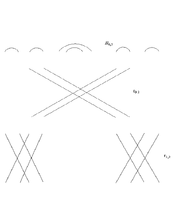
Figure 4: The $\phi$-images of the elements $t_{0,2}$ and $t_{1,2}$.

It is easy to check that the generators of $A_{i,p}$ and $L_{i}$, and hence the whole group $N_{i,p}$ leaves $B_{i,p}$ invariant. The next lemma shows that $N_{i,p}$ is the full stabilizer of $B_{i,p}$ in $W({\rm C}_{n})$.

Lemma 6.4.

The subgroup of $W({\rm C}_{n})$ generated by $\{t_{j,p}\}_{j=0}^{q-1}$ is isomorphic to $W({\rm C}_{q})$ and the cardinality of $A_{i,p}$ is $2^{i}p!q!$. Moreover, $L_{i}$ is isomorphic to $W({\rm C}_{n-i})$. Furthermore, $N_{i,p}$ is the stabilizer of $B_{i,p}$ in $W({\rm C}_{n})$ and isomorphic to $A_{i,p}\times L_{i}$.

Proof.

Put

$$A=\langle r_{0},r_{1},\ldots,r_{p-1}\rangle,$$

$$B=\langle t_{0,p},t_{1,p},\ldots,t_{q-1,p}\rangle,$$

$$C=\langle r_{p+1},r_{p+3},\ldots,r_{i-1}\rangle.$$

Being a parabolic subgroup of type ${\rm C}_{p}$, the group $A$ is isomorphic to $W({\rm C}_{p})$. Since the supports of the simple reflections involved in $A$ lie in $\{0,\ldots,p-1\}$ and those of $B\cup C$ lie in $\{p+1,\ldots,i\}$, each element of $A$ commutes with each element of $B\cup C$. Now we claim that $B$ is isomorphic to $W({\rm C}_{q})$. Ignoring the $2p$ vertical strands in the middle of generators of $B$ in ${\rm BrM}({\rm A}_{2n-1})$, and comparing them with canonical generators of $W({\rm C}_{q})$ in ${\rm BrM}({\rm A}_{2q-1})$ gives an easy pictorial proof of our claim.

Consider the diagrams of elements of $B$ and $C$ in ${\rm BrM}({\rm A}_{2n-1})$. Each diagram of $B$ only has non-crossing strands starting from $(n-k-1,1)$ and $(n-k+1,1)$, for $k=p+1$, $p+3,\ldots,i-1$, which can never occur in nontrivial elements of $C$. Hence $B\cap C=\{1\}$. For the generators of $B$ and $C$, the following equations hold.

$$t_{0,p}r_{p+2k-1}t_{0,p} = r_{p+2k-1},\,\mbox{for }\,1\leq k\leq q$$

$$t_{k,p}r_{p+2k-1}t_{k,p} = r_{p+2k+1},\,\mbox{for }\,1\leq k\leq q$$

$$t_{s,p}r_{p+2k-1}t_{s,p} = r_{p+2k-1},\,\mbox{for }1\leq s,\,k\leq q,\,\mbox{and}\,|s-k|>1.$$

Therefore the subgroup $BC$ in $W({\rm C}_{n})$ is the semiproduct of $C$ and $B$ with $C$ normal. Consider the diagrams of elements of $BC$ and $A$ in ${\rm Br}({\rm A}_{2n-1})$. Each element in $BC$ keeps the $2p$ strands in the middle invariant, but each element of $A$ keeps the left $2n-2p+2$ strands invariant. Therefore $A\cap BC=\{1\}$. Thus, $A_{i,p}=BC\times A$, and hence

$$|A_{i,p}|=|B||C||A|=2^{i}p!q!.$$

The reflections $y_{i+1}$, $r_{i}$, $r_{i+1}$, $\ldots$, $r_{n-1}$ have roots $\beta_{0}+2\beta_{1}+\cdots+2\beta_{i}$, $\beta_{i+1}$, $\ldots$, $\beta_{n-1}$, respectively, which form a simple root system of type ${\rm C}_{n-i}$. Therefore the subgroup $L_{i}$ is isomorphic to $W({\rm C}_{n-i})$.

In the Coxeter diagram ${\rm A}_{2n-1}$ we see that $A_{i,p}\cap L_{i}=1$ and all elements in $L_{i}$ commute with all elements in $A_{i,p}$, so $N_{i,p}$ is the direct product of $L_{i}$ and $A_{i,p}$. This gives

$$|D_{i,p}| = \frac{|W({\rm C}_{n})|}{|A_{i,p}||L_{i}|}=\frac{n!}{p!q!(n-i)!}.$$

By Lagrange’s Theorem, the cardinality of $D_{i,p}$ is equal to the size of the $W({\rm C}_{n})$-orbit of $B_{i,p}$. Therefore by Lemma 6.1, $N_{i,p}$ is the stabilizer of $B_{i,p}$ in $W({\rm C}_{n})$. ∎

The study of the stabilizer of $B_{i,p}$ will now be used to rewrite products of $b_{p,i,p^{\prime}}$ with elements of $W({\rm C}_{n})$. The result is in Lemma 6.6 and needs the following special cases.

Lemma 6.5.

Let $i\in\{0,\ldots,n\}$ and $p\in\{0,\ldots,i\}$ with $i-p$ even.

1. For each $r\in A_{i,p}$ we have $rb_{p,i,i}=b_{p,i,i}$.

2. For each $v\in L_{i}$ we have $ve_{i,p}=e_{i,p}v$ and $vb_{p,i,i}=b_{p,i,i}v$.

Proof.

(ii). By Lemma 4.3 and Definition 2.1, the two equations hold for the generators of $L_{i}$. Therefore they hold for each element of $L_{i}$.

(i). The roots $\beta_{j}$ and $r_{j}r_{j-1}\cdots r_{1}\beta_{0}$ are as in Proposition 5.9(iii), so

$$r_{j}z_{j}z_{j+1} = (r_{j}z_{j}r_{j}z_{j})r_{j}\overset{(\ref{0.1.19})}{=}z_{j}(e_{j}z_{j}r_{j})\overset{(\ref{0.1.18})}{=}z_{j}e_{j}z_{j}\overset{(\ref{4.1.5})}{=}z_{j}r_{j}z_{j}r_{j}=z_{j}z_{j+1}.$$

This proves that (i) is satisfied with $r=r_{j}$ for $j=0,\ldots,p-1$. For the choices $r=r_{p+2k-1}$ for $k=1,\ldots,q$ this is straightforward. Moreover, $t_{0,p}e_{p+1}=y_{p+1}(r_{p+1}y_{p+1}e_{p+1})=y_{p+1}y_{p+1}e_{p+1}=e_{p+1}$, and

$$t_{k,p}e_{p+2k-1}e_{p+2k+1} = r_{p+2k}r_{p+2k+1}r_{p+2k-1}r_{p+2k}e_{p+2k-1}e_{p+2k+1}$$

$$\overset{(\ref{0.1.13})}{=} (r_{p+2k}r_{p+2k+1}e_{p+2k})e_{p+2k-1}e_{p+2k+1}$$

$$\overset{(\ref{0.1.13})+(\ref{0.1.9})}{=} (e_{p+2k+1}e_{p+2k}e_{p+2k+1})e_{p+2k-1}$$

$$\overset{(\ref{3.1.5})}{=} e_{p+2k-1}e_{p+2k+1}.$$

So (i) holds for all generators of $A_{i,p}$ and hence for all of $A_{i,p}$. ∎

Lemma 6.6.

Suppose $r\in W({\rm C}_{n})$. Let $i\in\{0,\ldots,n\}$ and $p\in\{0,\ldots,i\}$ with $i-p$ even.

1. There are $u\in D_{i,p}$ and $v\in L_{i}$ such that $rb_{p,i,i}=ub_{p,i,i}v$.

2. There are $u^{\prime}\in D_{i,p}^{{\rm op}}$ and $v^{\prime}\in L_{i}$ such that $b_{i,i,p}r=v^{\prime}b_{i,i,p}u^{\prime}$.

Proof.

Let $r\in W({\rm C}_{n})$. By Lemma 6.4 and Definition 6.3 for $D_{i,p}$, there exist $u\in D_{i,p}$, $v\in L_{i}$, and $a\in A_{i,p}$ such that $r=uva$. By Lemma 6.5,

$$rb_{p,i,i} = uvab_{p,i,i}=uvb_{p,i,i}=ub_{p,i,i}v.$$

The second statement follows by applying Proposition 4.2 to (i). ∎

Our next step towards a normal form for elements of ${\rm BrM}({\rm C}_{n})$ is to describe products of elements from $W({\rm C}_{n})b_{p,i,p^{\prime}}W({\rm C}_{n})$ with generators $e_{j}$. To this end we first prove two useful equalities.

Lemma 6.7.

In ${\rm Br}({\rm C}_{n})$, the following hold for $i\in\{2,\ldots,n-1\}$.

$$e_{i}z_{i+1} = e_{i}z_{i},$$ (6.1)

$$e_{i-1}z_{i+1}z_{i}z_{i-1} = r_{i}r_{i-1}e_{i}z_{i}z_{i+1}z_{i-1},$$ (6.2)

$$e_{i}z_{i+1}z_{i}e_{i} = \delta^{2}e_{i}.$$ (6.3)

Proof.

By Lemma 5.9(iii), $e_{i}z_{i+1}\overset{(\ref{df:zn})}{=}e_{i}r_{i}z_{i}r_{i}\overset{(\ref{0.1.4})}{=}e_{i}z_{i}r_{i}\overset{(\ref{0.1.18})}{=}e_{i}z_{i}$. This proves (6.1).

Now (6.3) follows from Lemma 5.9(i) as

$$e_{i}z_{i+1}z_{i}e_{i} \overset{(\ref{ezez1})}{=} e_{i}z_{i}^{2}e_{i}=\delta e_{i}z_{i}e_{i}\overset{(\ref{0.1.16})}{=}\delta^{2}e_{i}.$$

As for (6.2), note that (2.13) and Proposition 5.9(iii) give $z_{i-1}e_{i-1}z_{i-1}=r_{i-1}z_{i-1}r_{i-1}z_{i-1}=z_{i}z_{i-1}$. Hence

$$r_{i-1}r_{i}e_{i-1}z_{i+1}z_{i}z_{i-1} \overset{(\ref{0.1.13})}{=} e_{i}e_{i-1}z_{i+1}z_{i}z_{i-1}\overset{\ref{X_n}}{=}e_{i}z_{i+1}e_{i-1}z_{i}z_{i-1}\overset{\rm{(\ref{ezez1})}}{=}\delta e_{i}z_{i}e_{i-1}z_{i-1}$$

$$\overset{\rm{(\ref{ezez1})}+\ref{prop:opp}}{=} \delta e_{i}z_{i-1}e_{i-1}z_{i-1}=\delta e_{i}z_{i}z_{i-1}\overset{\rm{(\ref{ezez1})}}{=}e_{i}z_{i+1}z_{i}z_{i-1},$$

and the equation follows by left multiplication with $r_{i}r_{i-1}$. ∎

The detailed information stated in the last sentence of the following proposition will be needed for the proof of cellularity of ${\rm Br}({\rm C}_{n},R,\delta)$ in the next section.

Proposition 6.8.

Let $i,p,p^{\prime}$ be natural numbers with $0\leq p,p^{\prime}\leq i\leq n$ and $i-p$ and $i-p^{\prime}$ even. For each root $\beta\in\Psi^{+}$, there are $h\in\{i,i+1,i+2\}$, $k$, $m$, $m^{\prime}\in\mathbb{N}$, $u\in D_{h,m}$, $w\in D_{h,m^{\prime}}^{{\rm op}}$, and $v\in L_{h}$ such that

$$e_{\beta}b_{p,i,p^{\prime}}=\delta^{k}ub_{m,h,m^{\prime}}vw.$$

Moreover, if $h=i$, then $w=1$ and $m^{\prime}=p^{\prime}$, while $k$, $u$, and $v$ do not depend on $p^{\prime}$.

Proof.

We first sketch the general idea of proof. There are only two possible root lengths in the Coxeter root system $\Psi$ of type ${\rm C}_{n}$. We call $\beta\in\Psi$ short if $(\beta,\beta)=1$ and long otherwise, in which case $(\beta,\beta)=2$. In each case, only one root needs to be considered, for all other roots of the same length are conjugate to this particular one under the natural action of $W({\rm C}_{n})$, and Lemma 6.6 can be applied to reduce to the representative root.

The top of $b_{p,i,p^{\prime}}$ is the admissible set $B_{i,p}$ displayed in Figure 3.

First suppose $\beta$ is long. Then $\beta$ can be written as $\beta_{0}+2\beta_{1}+\cdots+2\beta_{t-1}$, for some $1\leq t\leq n$, and so $e_{\beta}=z_{t}$. We will distinguish cases according to relations among $t$, $i$, and $p$, and apply induction on $t$ and $i$. In Figure 5 the roots of the Cases L1, L2, and L3 are displayed as the top, middle, and bottom horizontal strand, respectively.

Figure 5: Horizontal strands representing the three cases for a long root $\beta$.

Case L1. Suppose $t\geq i+1$. For any $t>i+1$, we have $z_{t}=sz_{i+1}s^{-1}$, where $s=r_{t-1}\cdots r_{i+1}$. This implies that $z_{t}b_{p,i,p^{\prime}}=sz_{i+1}b_{p,i,p^{\prime}}s^{-1}$, with $s\in L_{i}$. Lemmas 6.6 and 6.5 can be used to reduce this case to the case where $t=i+1$.

If $p=p^{\prime}=i$, then $e_{i,p}=e_{i,p^{\prime}}=1$ and $z_{i+1}b_{i}=b_{i+1}$ by the definition of $b_{i}$ in (5.1), as required.

If $p\neq i=p^{\prime}$, it suffices to prove the equation

$$z_{i+1}b_{p,i,i}=rb_{p+1,i+1,i+1},$$

with $r$ in the subgroup of $W({\rm C}_{n})$ generated by $r_{0},r_{1},\ldots,r_{i}$. We proceed by induction on $i$. In view of Lemma 6.7, (below IH is short for Inductive Hypothesis),

$$z_{i+1}b_{p,i,i} \overset{(\ref{eq:bi})+(\ref{fip})}{=} z_{i+1}e_{i-1}e_{i-2,p}z_{i}z_{i-1}b_{i-2}\overset{\ref{X_n}}{=}e_{i-1}z_{i+1}z_{i}z_{i-1}e_{i-2,p}b_{i-2}$$

$$\overset{(\ref{ezzz})}{=} r_{i}r_{i-1}e_{i}z_{i}z_{i+1}z_{i-1}e_{i-2,p}b_{i-2}\overset{\ref{X_n}}{=}r_{i}r_{i-1}e_{i}(z_{i-1}b_{p,i-2,i-2})z_{i}z_{i+1}$$

$$\overset{{\rm IH}}{=} r_{i}r_{i-1}e_{i}gb_{p+1,i-1,i-1}z_{i}z_{i+1}=r_{i}r_{i-1}ge_{i}b_{p+1,i-1,i-1}z_{i}z_{i+1}$$

$$= r_{i}r_{i-1}gb_{p+1,i+1,i+1},$$

where $g$ is an element of the subgroup of $W({\rm C}_{n})$ generated by $r_{0},r_{1},\ldots,r_{i-2}$. Hence the claim holds.

The case $p=i\neq p^{\prime}$ now follows by use of Proposition 4.2.

If $p$, $p^{\prime}\neq i$ then, by the above,

$$z_{i+1}b_{p,i,p^{\prime}} = re_{i+1,p+1}b_{i+1}e_{i,p^{\prime}}=re_{i+1,p+1}b_{i}e_{i,p^{\prime}}z_{i+1}=re_{i+1,p+1}b_{i+1}e_{i+1,p^{\prime}+1}r^{\prime}$$

$$= rb_{p+1,i+1,p^{\prime}+1}r^{\prime},$$

where $r$, $r^{\prime}\in W({\rm C}_{n})$. By Lemma 6.5, we conclude that this expression can be written in the required form with $h=i+1$.

Case L2. Next suppose $p+1\leq t<i+1$. By definition of $z_{i}$,

$$z_{i-1} = r_{i-1}z_{i}r_{i-1},$$

$$z_{i-2} = r_{i-2}r_{i-3}r_{i-1}r_{i-2}z_{i}r_{i-2}r_{i-3}r_{i-1}r_{i-2},$$

with $r_{i-1}$, $r_{i-2}r_{i-3}r_{i-1}r_{i-2}\in A_{i,p}$. By induction on $t$, we can find $r\in A_{i,p}$ such that $z_{t}=rz_{i}r^{-1}$. By Lemma 6.5,

$$e_{\beta}b_{p,i,p^{\prime}}=z_{t}b_{p,i,p^{\prime}}=rz_{i}r^{-1}b_{p,i,p^{\prime}}=rz_{i}b_{p,i,p^{\prime}}.$$

In view of Lemma 6.6, this reduces the problem to rewriting $z_{i}b_{p,i,p^{\prime}}$ in the required form.

Now

$$z_{i}e_{i-1}z_{i}z_{i-1} = (r_{i-1}z_{i-1}r_{i-1}e_{i-1})z_{i-1}z_{i}\overset{(\ref{0.1.4})+(\ref{4.1.2})}{=}z_{i-1}e_{i-1}z_{i-1}z_{i}$$

$$\overset{(\ref{0.1.19})}{=} (r_{i-1}z_{i-1}r_{i-1})z_{i-1}z_{i}=z_{i}z_{i-1}z_{i}$$

$$= \delta z_{i}z_{i-1},$$

so

$$z_{i}b_{p,i,i} \overset{(\ref{fip})}{=} z_{i}e_{i-1}e_{i-2,p}z_{i-1}z_{i}b_{i-2}\overset{\ref{X_n}}{=}z_{i}e_{i-1}z_{i-1}z_{i}e_{i-2,p}b_{i-2}$$

$$= \delta z_{i-1}z_{i}b_{p,i-2,i-2},$$

by the claim of Case L1 and Lemma 6.6, the above can be written as $ub_{p+2,i,i}v$ with $u\in D_{i,p+2}$ and $v\in L_{i}$, and so the proposition holds in this case as $z_{i}b_{p,i,p^{\prime}}=ub_{p+2,i,p^{\prime}}v$.

Case L3. We remain with the case where $1\leq t\leq p$. We have

$$z_{t}b_{p,i,p^{\prime}} = e_{i,p}z_{t}b_{i}e_{i,p^{\prime}}=\delta e_{i,p}b_{i}e_{i,p^{\prime}}=\delta b_{p,i,p^{\prime}},$$

and so the proposition holds with $h=i$.

We next consider the case where $\beta$ is a short root, which means $\beta=\beta_{s}+\beta_{s+1}+\cdots+\beta_{t}$ with $0<s\leq t\leq n-1$ or $\beta=\beta_{0}+2\beta_{1}+\cdots+2\beta_{s-1}+\beta_{s}+\beta_{s+1}+\cdots+\beta_{t}$ with $0\leq s\leq t\leq n-1$. We will distinguish seven cases by values of $s$ and $t$ corresponding to the horizontal strands of Figure 6. The seven cases occur in the order from top to bottom.

Figure 6: Strands corresponding to 7 possibilities for the long root $\beta$.

Case S1. Suppose that $\beta$ is a linear combination of $\beta_{j}$ $(j=i+1,\ldots,n-1)$. Then, by Lemma 6.7,

$$e_{i+1}b_{p,i,p^{\prime}} = e_{i,p}e_{i+1}b_{i}e_{i,p^{\prime}}\overset{(\ref{ezze})}{=}\delta^{-2}e_{i,p}(e_{i+1}z_{i+2}z_{i+1}e_{i+1})b_{i}e_{i,p^{\prime}}$$

$$= \delta^{-2}e_{i,p}e_{i+1}z_{i+2}z_{i+1}b_{i}e_{i+1}e_{i,p^{\prime}}$$

$$\overset{(\ref{eq:bi})+(\ref{fip})}{=} \delta^{-2}e_{i+2,p}b_{i+2}e_{i+2,p^{\prime}}=\delta^{-2}b_{p,i+2,p^{\prime}}.$$

At the same time, for any such $\beta\in\Psi^{+}$, there exists an element $r\in L_{i}$ such that $\beta=r\beta_{i+1}$, thus $e_{\beta}=re_{i+1}r^{-1}$. Now $e_{\beta}b_{p,i,p^{\prime}}=\delta^{-2}rb_{p,i+2,p^{\prime}}r^{-1}$, and hence the proposition holds with $h=i+2$.

Case S2. Suppose $\beta=\beta_{s}+\beta_{s+1}+\cdots+\beta_{t}$, with $p\leq s\leq i\leq t\leq n-1$.

If $p=i$, then $e_{i,p}=1$. First, consider the case $t=s=i$. Since

$$e_{i}z_{i+1}z_{i} \overset{(\ref{ezez1})}{=} e_{i}z_{i}z_{i}\overset{\ref{lem:rel}(i)}{=}\delta e_{i}z_{i},$$

the use of the claim of Case L1 and Proposition 4.2 gives the existence of an element $r\in W({\rm C}_{n})$ such that

$$e_{i}b_{i,i,p^{\prime}} = \delta^{-1}e_{i}z_{i}b_{i}e_{i,p^{\prime}}\overset{\ref{lem:rel}(i)}{=}\delta^{-1}e_{i}z_{i+1}b_{i}e_{i,p^{\prime}}\overset{\ref{X_n}}{=}\delta^{-1}e_{i}b_{i,i,p^{\prime}}z_{i+1}$$

$$\overset{{\rm L1}}{=} \delta^{-1}e_{i}b_{i+1,i+1,p^{\prime}}r=\delta^{-1}b_{i-1,i+1,p^{\prime}}r,$$

as required.

If $t\neq s$, then $e_{\beta}=r_{\beta^{\prime\prime}}r_{\beta^{\prime}}e_{i}r_{\beta^{\prime}}r_{\beta^{\prime\prime}}$, where $\beta^{\prime}=\beta_{s}+\cdots+\beta_{i-1}$, $\beta^{\prime\prime}=\beta_{i+1}+\cdots+\beta_{t}$, which implies that $r_{\beta^{\prime}}\in A_{i,p}$, $r_{\beta^{\prime\prime}}\in L_{i}$, and hence $e_{\beta}b_{i}e_{i,p^{\prime}}=r_{\beta^{\prime\prime}}r_{\beta^{\prime}}e_{i}b_{i}e_{i,p^{\prime}}r_{\beta^{\prime\prime}}$. As in the argument for $e_{i}b_{i,i,p^{\prime}}$ above, this can be written in the required form with $h=i+1$.

On the other hand if $p\neq i$ , then $e_{i,p}\neq 1$. Therefore for $\beta=\beta_{s}+\beta_{s+1}+\cdots+\beta_{t}$, with $p\leq s\leq i\leq t\leq n-1$, since there is some $l\in\{p+1,p+3,\ldots,i-1\}$, such that $e_{\beta}e_{l}=r_{l}r_{\beta}e_{l}$, implying that $e_{\beta}e_{i,p}=r_{l}r_{\beta}e_{i,p}$ and $e_{\beta}b_{p,i,p^{\prime}}=r_{l}r_{\beta}b_{p,i,p^{\prime}}$. By Lemma 6.6, the proposition holds with $h=i$.

Case S3. Suppose $\beta=\beta_{s}+\beta_{s+1}+\cdots+\beta_{t}$ or $\beta=\beta_{0}+2\beta_{1}+\cdots+2\beta_{s-1}+\beta_{s}+\cdots+\beta_{t}$ with $0<s\leq p$ and $i\leq t\leq n-1$.

First consider $\beta=\beta_{p}+\cdots+\beta_{i}$. Following the argument for $e_{i}z_{i+1}z_{i}=\delta e_{i}z_{i}$ in the above case, we find that $e_{\beta}z_{i+1}z_{i}=\delta e_{\beta}z_{i}$ holds, which implies

$$e_{\beta}b_{p,i,p^{\prime}}=e_{i,p}e_{\beta}b_{i}e_{i,p^{\prime}}=\delta^{-1}e_{i,p}e_{\beta}b_{i+1}e_{i,p^{\prime}}.$$ (6.4)

Observe that

$$r_{i-1}r_{i}e_{\beta}e_{i-1} = e_{\beta-\beta_{i}-\beta_{i-1}}r_{i-1}r_{i}e_{i-1}r_{i}r_{i-1}r_{i-1}r_{i}\overset{(\ref{0.1.15})}{=}e_{\beta-\beta_{i}-\beta_{i-1}}e_{i}r_{i-1}r_{i},$$

$$\mbox{and }\,r_{i-1}r_{i}b_{i+1} \overset{\ref{lm:rfp}}{=} b_{i+1}.$$

Therefore (6.4) can be written as

$$\delta^{-1}e_{i,p}e_{\beta}b_{i+1}e_{i,p^{\prime}} = \delta^{-1}(e_{i-1}r_{i}r_{i-1})e_{i-2,p}e_{\beta-\beta_{i}-\beta_{i-1}}b_{i+1}e_{i,p^{\prime}}$$

$$\overset{(\ref{0.1.15})}{=} \delta^{-1}r_{i}r_{i-1}e_{i}e_{i-2,p}e_{\beta-\beta_{i}-\beta_{i-1}}b_{i+1}e_{i,p^{\prime}}$$

$$= \delta^{-1}r_{i}r_{i-1}e_{i}(e_{\beta-\beta_{i}-\beta_{i-1}}e_{i-2,p}b_{i-2})z_{i-1}z_{i}z_{i+1}e_{i,p^{\prime}}.$$

By induction on $i$, we can use an argument as in the claim of Case S1, and the above can be written as

$$\delta^{-1}r_{i}r_{i-1}e_{i}ge_{i-1,p-1}b_{i-1}z_{i-1}z_{i}z_{i+1}e_{i,p^{\prime}} = r_{i}r_{i-1}ge_{i}e_{i-1,p-1}b_{i-1}z_{i}z_{i+1}e_{i,p^{\prime}}$$

$$= r_{i}r_{i-1}ge_{i+1,p-1}b_{i}z_{i+1}e_{i,p^{\prime}}$$

$$= r_{i}r_{i-1}ge_{i+1,p-1}b_{i,i,p^{\prime}}z_{i+1},$$

where $g\in W({\rm C}_{n})$ is a product of elements from $r_{0},r_{1},\ldots,r_{i-2}$. By Case L1 and Proposition 4.2, the proposition holds with $h=i+1$.

We return to the general setting of Case S3. Then there exists $r^{\prime}\in L_{i}$ and $r^{\prime\prime}\in A_{i,p}$ such that $r^{\prime}r^{\prime\prime}\hat{\beta}=\beta$, with $\hat{\beta}=\beta_{p}+\cdots+\beta_{i}$. Then

$$e_{\beta}b_{p,i,p^{\prime}}=r^{\prime}r^{\prime\prime}e_{\hat{\beta}}b_{p,i,p^{\prime}}r^{\prime},$$

hence the proposition holds in Case S3 due to Lemma 6.6.

Case S4. If $\beta=\beta_{0}+2\beta_{1}+\cdots+2\beta_{s-1}+\beta_{s}+\cdots+\beta_{t}$ with $p\leq s\leq i\leq t\leq n-1$, and let $\beta^{\prime}=\beta_{s}+\cdots+\beta_{t}$. Then $e_{\beta}=y_{s}e_{\beta^{\prime}}y_{s}.$ When $p=i=s$, we see that $y_{s}\in A_{i,p}$; when $p\neq i$, there is some $l\in\{p+1,p+3,\ldots,i-1\}$, such that $e_{\beta}e_{l}=r_{l}r_{\beta}e_{l}$. This brings us back to the argument of Case S2.

Case S5. If $\beta=\beta_{0}+2\beta_{1}+\cdots+2\beta_{s}+\beta_{s+1}+\cdots+\beta_{t}$, with $i<s\leq t\leq n-1$, then $\beta=y_{s+1}\beta^{\prime}$, with $\beta^{\prime}=\beta_{s+1}+\beta_{s+2}+\cdots+\beta_{t}$, and $y_{s+1}\in L_{i}$. Therefore

$$e_{\beta}b_{p,i,p^{\prime}}=y_{s+1}(e_{\beta^{\prime}}b_{p,i,p^{\prime}})y_{s+1},$$

and we are back in Case S1.

Case S6. If $\beta=\beta_{0}+2\beta_{1}+\cdots+2\beta_{s}+\beta_{s+1}+\cdots+\beta_{t}$ or $\beta=\beta_{s}+\beta_{s+1}+\cdots+\beta_{t}$, with $0\leq s\leq t$ and $p\leq t\leq i-1$, then there must be some $e_{j}\in\{e_{p+2j-1}\}_{j=1}^{(i-p)/2}$ such that $\beta$ is not orthogonal to $\beta_{j}$, or $\{\beta,\beta_{j}\}$ is not admissible, or $\beta=\beta_{j}$. Then, by Lemma 5.9, there exists $r\in W({\rm C}_{n})$ such that $e_{\beta}e_{i,p}=re_{i,p}$ or $e_{\beta}e_{i,p}=\delta re_{i,p}$. This implies that the proposition holds with $h=i$.

Case S7. If $\beta$ can be written as a linear combination of $\{\beta_{j}\}_{j=0}^{p-1}$, then $\beta$ is conjugate to $\beta_{p-1}$ under the subgroup of $A_{i,p}$ generated by $\{r_{j}\}_{j=0}^{p-1}$. Then we can find a $r\in A_{i,p}$ such that $r\beta_{p-1}=\beta$, which implies

$$e_{\beta}b_{p,i,p^{\prime}} = re_{p-1}r^{-1}b_{i,i,p^{\prime}}\overset{\ref{lm:rfp}(i)}{=}re_{p-1}b_{i,i,p^{\prime}}=rb_{p-2,i,p^{\prime}},$$

so the proposition holds with $h=i$ due to Lemma 6.6. ∎

Theorem 6.9.

Each element in the monoid ${\rm BrM}({\rm C}_{n})$ can be written as

$$\delta^{k}ub_{p,i,p^{\prime}}vw^{{\rm op}},$$

where $k\in\mathbb{Z}$ and $i,p,p^{\prime}\in\{0,\ldots,n\}$ with $i-p$ and $i-p^{\prime}$ even, $u\in D_{i,p}$, $v\in L_{i}$, and $w\in D_{i,p^{\prime}}$. In particular, ${\rm Br}({\rm C}_{n})$ is free of rank at most $a_{2n}$.

Proof.

Let $U$ be the set of elements of ${\rm BrM}({\rm C}_{n})$ of the indicated form. We show that $U$ is invariant under left multiplication by generators of ${\rm BrM}({\rm C}_{n})$. To this end, consider an arbitrary element $a=\delta^{k}ub_{p,i,p^{\prime}}vw^{{\rm op}}$ of $U$. Obviously $\delta^{\pm 1}a\in U$. Without loss of generality, we may take $k=0$.

Let $r\in W({\rm C}_{n})$. By Lemma 6.6 applied to $ru$ there are $u^{\prime}\in D_{i,p}$ and $v^{\prime}\in L_{i}$ such that $ra=rub_{p,i,p^{\prime}}vw^{{\rm op}}$. By Lemma 6.5, this is equal to $u^{\prime}b_{p,i,p^{\prime}}v^{\prime}vw^{{\rm op}}$ and, as $v^{\prime}v\in L_{i}$, the set $U$ is invariant under left multiplication by Weyl group elements.

Finally, consider the generator $e_{j}$ of ${\rm BrM}({\rm C}_{n})$. Writing $\beta=u^{{\rm op}}\alpha_{j}$ we have $e_{j}a=e_{j}ub_{p,i,p^{\prime}}vw^{{\rm op}}=ue_{\beta}b_{p,i,p^{\prime}}vw^{{\rm op}}$ and by Proposition 6.8 this belongs to $U$ again.

Now, by Proposition 4.2 we also find that $U$ is invariant under right multiplication by generators. This proves that $U$ is invariant under both left and right multiplication by any generator of ${\rm BrM}({\rm C}_{n})$. As it contains the identity $(b_{0,0,0})$, it follows that $U$ coincides with the whole monoid.

As for the last assertion of the theorem, observe that freeness of ${\rm Br}({\rm C}_{n})$ over $\mathbb{Z}[\delta^{\pm 1}]$ is immediate from the fact that it is a monomial algebra with a finite number of generators. By the first assertion, its rank is at most

$$\sum_{i=0}^{n}\left(\sum_{p\equiv i\pmod{2}}|D_{i,p}|\right)^{2}\cdot|L_{i}|.$$

By Lemma 6.1, the cardinality of $D_{i,p}$ is $n!/(p!q!(n-i)!)$, where $q=(i-p)/2$, and, by Lemma 6.4, $L_{i}$ is isomorphic to $W({\rm C}_{n-i})$, which has $2^{n-i}(n-i)!$ elements. Therefore, the rank of ${\rm Br}({\rm C}_{n})$ over $\mathbb{Z}[\delta^{\pm 1}]$ is at most

$$\sum_{i}\left(\sum_{p,q:p+2q=i}\frac{n!}{p!q!(n-i)!}\right)^{2}2^{n-i}(n-i)!.$$

Corollary 6.2 gives that this sum is equal to $a_{2n}$. ∎

We are now ready to prove Theorem 1.1. Theorem 6.9 shows that ${\rm Br}({\rm C}_{n})$ is free of rank at most $a_{2n}$. By Proposition 5.16, the homomorphism $\phi:{\rm Br}({\rm C}_{n})\to{\rm SBr}({\rm A}_{2n-1})$ is surjective, so the rank of ${\rm Br}({\rm C}_{n})$ is at least the rank of ${\rm SBr}({\rm A}_{2n-1})$, which is known to be $a_{2n}$ by Corollary 2.7. Thus, the ranks of ${\rm Br}({\rm C}_{n})$ and ${\rm SBr}({\rm A}_{2n-1})$ coincide and $\phi$ is an isomorphism.

7 Further properties of type ${\rm C}$ algebras

In this section we prove that the algebra ${\rm BrM}({\rm C}_{n},R,\delta)$ is cellular, in the sense of Graham and Lehrer [10], provided $R$ is an integral domain containing the inverse to $2$. The proof given here runs parallel to the proof of the corresponding result for ${\rm D}_{n}$ in [5, Section 6]. We finish by discussing a few more desirable properties of the newly found Brauer algebras.

Recall from [10] that an associative algebra ${A}$ over a commutative ring $R$ is cellular if there is a quadruple $(\Lambda,T,C,*)$ satisfying the following three conditions.

• $\Lambda$ is a finite partially ordered set. Associated to each $\lambda\in\Lambda$, there is a finite set $T(\lambda)$. Also, $C$ is an injective map

  $$\coprod_{\lambda\in\Lambda}T(\lambda)\times T(\lambda)\rightarrow{A}$$

  whose image is an $R$-basis of ${A}$.

• The map $*:{A}\rightarrow{A}$ is an $R$-linear anti-involution such that $C(x,y)^{*}=C(y,x)$ whenever $x,y\in T(\lambda)$ for some $\lambda\in\Lambda$.

• If $\lambda\in\Lambda$ and $x,y\in T(\lambda)$, then, for any element $a\in{A}$,

  $$aC(x,y)\equiv\sum_{u\in T(\lambda)}r_{a}(u,x)C(u,y)\ \ \ {\rm mod}\ {A}_{<\lambda},$$

  where $r_{a}(u,x)\in R$ is independent of $y$ and where ${A}_{<\lambda}$ is the $R$-submodule of ${A}$ spanned by $\{C(x^{\prime},y^{\prime})\mid x^{\prime},y^{\prime}\in T(\mu)\mbox{ for }\mu<\lambda\}$.

Such a quadruple $(\Lambda,T,C,*)$ is called a cell datum for ${A}$. We will describe such a quadruple for ${\rm Br}({\rm C}_{n},R,\delta)$.

For $*$ we will use the anti-involution ${\rm op}$ determined in Proposition 4.2. Let $i\in\{0,\ldots,n\}$. By Theorem 6.9, each element in the monoid ${\rm BrM}({\rm C}_{n})$ can be written in the form

$$\delta^{k}ub_{p,i,p^{\prime}}vw^{{\rm op}},$$

where $k\in\mathbb{Z}$ and $i,p,p^{\prime}\in\{0,\ldots,n\}$ are such that $i-p$ and $i-p^{\prime}$ are even, $u\in D_{i,p}$, $v\in L_{i}$, and $w\in D_{i,p^{\prime}}$. As the coefficient ring $R$ is an integral domain containing the inverse of $2$, it satisfies the conditions of [8, Theorem 1.1], so by [8, Corollary 3.2] the group rings $R[L_{i}]$ $(i=0,\ldots,n)$ are all cellular. By Lemma 6.4, the subalgebra $RL_{i}$ of ${\rm Br}({\rm C}_{n},R,\delta)$ (with unit ${\hat{b}}^{(i)}$, see (5.6)) generated by $L_{i}$ is isomorphic to $R[L_{i}]$. Let $(\Lambda_{i},T_{i},C_{i},*_{i})$ be a cell datum for $RL_{i}$ an in [8]. Observe that the generators of $L_{i}$ in Definition 6.3 are fixed by ${\rm op}$, so $RL_{i}$ is ${\rm op}$-invariant. By [8, Section 3], $*_{i}$ is the map ${\rm op}$ on $RL_{i}$ and so $*_{i}$ is the restriction of ${\rm op}$ to $RL_{i}$.

The underlying poset $\Lambda$ will be $\{B_{i}\}_{i=0}^{n}$, as defined in (5.2). We say that $B_{i}>B_{j}$ if and only if $i<j$ or, equivalently, $B_{i}\subset B_{j}$. In particular, $\emptyset$ is the greatest element of $\Lambda$.

The set $T(B_{i})$ is taken to be the set of all triples $(u,e_{i,p},s)$ where $u\in D_{i,p}$ (see Definition 6.3), $p\in\{0,\ldots,i\}$ with $i-p$ even, and the product $e_{i,p}$ is given by (5.4), and $s\in T_{i}$. Clearly, this set is finite.

The map $C$ is given by $C((u,e_{i,p},s),(w,e_{i,p^{\prime}},t))=ue_{i,p}C_{i}(s,t)e_{i,p^{\prime}}w^{{\rm op}}$. By Lemma 6.5, $ub_{p,i,p^{\prime}}vw^{{\rm op}}=(ue_{i,p})(b_{i}v)(we_{i,p^{\prime}})^{{\rm op}}$, so the image of $C$ is a basis by Theorems 1.1 and 6.9, and the fact that $\{C_{i}(s,t)\mid s,t\in T_{i}\}$ is a basis for $RL_{i}$ (which is a consequence of (C1) for $(\Lambda_{i},T_{i},C_{i},*_{i})$). This gives a quadruple $(\Lambda,T,C,*)$ satisfying (C1).

For (C2) notice that $(ue_{i,p}C_{i}(s,t)e_{i,p^{\prime}}w^{{\rm op}})^{{{\rm op}}}=we_{i,p^{\prime}}C_{i}(s,t)^{{{\rm op}}}e_{i,p}u^{{\rm op}}$. Now $C_{i}(s,t)^{{{\rm op}}}=C_{i}(t,s)$, by the cellularity condition (C2) for $RL_{i}$ and so (C2) holds for the cell datum $(\Lambda,T,C,*)$.

Finally, we check condition (C3) for $(\Lambda,T,C,*)$. It suffices to consider the left multiplications by $r_{j}$ and $e_{j}$ of $ue_{i,p}C_{i}(s,t)e_{i,p^{\prime}}w^{{\rm op}}$. Up to linear combinations, we can replace the latter expression by $ue_{i,p}b_{i}ve_{i,p^{\prime}}w^{{\rm op}}$ for $v\in L_{i}$. Now, by Lemma 6.6 for $r_{j}$ and Proposition 6.8 for $e_{j}$ (note the product lies in ${\rm Br}({\rm C}_{n},R,\delta)_{<B_{i}}$ if $h>i$), (C3) holds for the cell datum $(\Lambda,T,C,*)$. Therefore we have now proved

Theorem 7.1.

Let $R$ be an integral domain with $2^{-1}\in R$. Then the quadruple $(\Lambda,T,C,*)$ is a cell datum for ${\rm Br}({\rm C}_{n},R,\delta)$, proving the algebra is cellular.

We continue by discussing some desirable properties of the Brauer algebra ${\rm Br}({\rm C}_{n})$. First of all, for any disjoint union $M$ of diagrams of type $Q$, for $Q$ a simply laced graph, and ${\rm C}_{k}$ for $k\in\mathbb{N}$, the Brauer algebra is defined as the direct product of the Brauer algebras whose types are the components of $X$. The next result states that parabolic subalgebras behave well.

Proposition 7.2.

Let $J$ be a set of nodes of the Dynkin diagram ${\rm C}_{n}$. Then the parabolic subalgebra of the Brauer algebra ${\rm Br}({\rm C}_{n})$, that is, the subalgebra generated by $\{r_{j},e_{j}\}_{j\in J}$, is isomorphic to the Brauer algebra of type $J$.

Proof.

In view of induction on $n-|J|$ and restriction to connected components of $J$, it suffices to prove the result for $J=\{1,\ldots,n-1\}$ and for $J=\{0,\ldots,n-2\}$. In the former case, the type is ${\rm A}_{n-1}$ and the statement follows from the observation that the symmetric diagrams without strands crossing the vertical line through the middle of the segments connecting the dots $(n,1)$ and $(n+1,1)$ are equal in number to the Brauer diagrams on the $2n$ nodes (realized to the left of the vertical line). In the latter case, the type is ${\rm C}_{n-1}$ and the statement follows from the observation that the symmetric diagrams with vertical strands from $(1,1)$ to $(1,0)$ and from $(2n,1)$ to $(2n,0)$ are equal in number to the symmetric diagrams related to ${\rm BrM}({\rm C}_{n-1})$. ∎

The reader may have wondered why the study of symmetric diagrams was restricted to type ${\rm A}_{m}$ for $m$ odd. The answer is that, if $m=2n$ is even, each symmetric diagram has a fixed vertical strand from the dot $(n,1)$ to $(n,0)$. The removal of this strand leads to an isomorphism of the algebra of the symmetric diagrams with ${\rm SBr}({\rm A}_{2n-1})$, and so this construction provides no new algebra. This is remarkable in that the root system obtained by projecting $\Phi$ onto the $\sigma$-fixed subspace of the reflection representation, as in Definition 5.1, leads to a root system of type ${\rm B}_{n}$ instead of ${\rm C}_{n}$.

On the other hand, the presentation by generators and relations given in Definition 2.1 suggests, at least when $\delta=1$, the definition of the Brauer algebra of type ${\rm B}_{n}$ as for ${\rm C}_{n}$, but with the roles of $0$ and $1$ reversed in defining relations (2.11)–(2.18). The dimensions for the Brauer algebras ${\rm Br}({\rm B}_{n},R,1)$ with $n\leq 5$ thus obtained were found to be

$n$	1	2	3	4	5
$a_{n}$	3	25	273	3801	66315

It is likely that these algebras emerge with a construction similar to the one given for ${\rm C}_{n}$ but with ${\rm A}_{2n-1}$ replaced by ${\rm D}_{n+1}$ and $\sigma$ by the diagram automorphism interchanging the two short end nodes. This will be the subject of further investigation.

At the time of writing of this paper, Chen [3] presented a definition of a generalized Brauer algebra of type ${\rm I}_{2}(m)$. For $m=4$, this type coincides with ${\rm C}_{2}$, but Chen’s algebra has dimension $2m+m^{2}=24$, whereas our ${\rm Br}({\rm C}_{2})$ has dimension 25.

8 Acknowledgments

The authors thank David Wales for his valuable comments and helpful suggestions during the preparation of this manuscript. Max Horn performed computations in GAP to explore the first few algebras of the series and their actions on admissible sets. We are very grateful for his help and enthusiastic support.

References

- [1] S. Bigelow, Braid groups are linear, Journal of the American Mathematical Society, 14 (2001), 471–486.
- [2] R. Brauer, On algebras which are connected with the semisimple continous groups, Annals of Mathematics, 38 (1937), 857–872.
- [3] Z. Chen, Algebras associated with pseudo reflection groups: A generalization of Brauer algebras, arXiv:1003.5280v1, March 2010.
- [4] A.M. Cohen, B. Frenk and D.B. Wales, Brauer algebras of simply laced type, Israel Journal of Mathematics, 173 (2009) 335–365.
- [5] A.M. Cohen, D.A.H. Gijsbers and D.B. Wales, The BMW Algebras of type Dn, arXiv:0704.2743, April 2007.
- [6] J. Crisp, Injective maps between Artin groups, in Geometric Group Theory Down Under, Lamberra 1996 (J. Cossey, C.F. Miller III, W.D. Neumann and M.Shapiro, eds.) De Gruyter, Berlin, 1999, 119–137.
- [7] T. tom Dieck, Quantum groups and knot algebra, Lecture notes, May 4, 2004.
- [8] M. Geck, Hecke algebras of finite type are cellular, Inventiones Mathematicae, 169 (2007), 501–517.
- [9] J. J. Graham, Modular representations of Hecke algebras and related algebras, Ph. D. thesis, University of Sydney, 1995.
- [10] J.J. Graham and G.I. Lehrer, Cellular algebras, Inventiones Mathematicae 123 (1996), 1–44.
- [11] B. Mühlherr, Coxeter groups in Coxeter groups, pp. 277–287 in Finite Geometry and Combinatorics (Deinze 1992). London Math. Soc. Lecture Note Series 191, Cambridge University Press, Cambridge, 1993.