Why are most molecular clouds not gravitationally bound?

Abstract

The most recent observational evidence seems to indicate that giant molecular clouds are predominantly gravitationally unbound objects. In this paper we show that this is a natural consequence of a scenario in which cloud-cloud collisions and stellar feedback regulate the internal velocity dispersion of the gas, and so prevent global gravitational forces from becoming dominant. Thus, while the molecular gas is for the most part gravitationally unbound, local regions within the denser parts of the gas (within the clouds) do become bound and are able to form stars. We find that the observations, in terms of distributions of virial parameters and cloud structures, can be well modelled provided that the star formation efficiency in these bound regions is of order 5 – 10 percent. We also find that in this picture the constituent gas of individual molecular clouds changes over relatively short time scales, typically a few Myr.

1 Introduction

The belief that molecular clouds are gravitationally bound objects has led to a long-standing problem in star formation. If clouds are bound, and if they collapse in of order a free-fall time, then the rate of star formation should be around two orders of magnitude greater than what is observed (Zuckerman & Evans, 1974). To circumvent this there have been two main approaches. Firstly, one can assume that molecular clouds undergo collapse on longer timescales, requiring that some process prevents, or at least slows their collapse. This could be magnetic fields and slow ambipolar diffusion (Shu et al., 1987; Basu & Mouschovias, 1994; Allen & Shu, 2000; Mouschovias et al., 2006; Shu et al., 2007), or microturbulence (Krumholz & McKee, 2005; Krumholz et al., 2006). However turbulence can also promote collapse on small scales (Klessen et al., 2000; Mac Low & Klessen, 2004), (including MHD turbulence Heitsch et al. 2001; Vázquez-Semadeni et al. 2005; Elmegreen 2007). Alternatively, in light of recent observational evidence, one can assume that clouds are typically short-lived entities (Hartmann et al., 2001; Elmegreen, 2002, 2007; Ballesteros-Paredes et al., 2007) and posit mechanisms which prevent most of the gas forming stars, such as stellar feedback and magnetic fields (Vázquez-Semadeni et al., 2005; Elmegreen, 2007; Price & Bate, 2008). However if the cloud is not globally bound in the first place, as suggested by recent observational evidence, we already ameliorate the disparity between the existence of short-lived molecular clouds and the global star formation rate.

The virial parameter of a molecular cloud is usually defined as

$$\alpha=\frac{5\sigma_{v}^{2}R}{GM}$$ (1)

(e.g. Bertoldi & McKee 1992; Dib et al. 2007), where $\sigma_{v}$ is the line of sight velocity dispersion and R is a measure of the radius of the cloud. If the cloud is in virial equilibrium, then $\alpha=1$ and $2T+W$=0 where $T$ is the kinetic and $W$ the gravitational energy, whereas $T+W=0$ corresponds to the zero energy configuration. The value of $\alpha$ is simply a measure of the ratio of kinetic to gravitational energies, and finding $\alpha$ both observationally and from simulations is highly uncertain, depending on the mass and radius determinations, and typically does not account for magnetic fields, surface terms or projection effects (Ballesteros-Paredes, 2006; Dib et al., 2007; Shetty et al., 2010). Thus the estimated value of $\alpha$ for one cloud may not predicate its consequent evolution, but the distribution of $\alpha$ gives an indication of the importance of gravity in a population of clouds, and whether they are predominantly bound or unbound.

In a recent observational study, Heyer et al. (2009) published revised estimates of molecular cloud masses, sizes and virial parameters from the previous seminal work by Solomon et al. (1987). Although they claim that molecular clouds are virialised, their plots seem to indicate that in fact most of the clouds are unbound (as also found by Heyer et al. 2001). In Fig. 1 (lower middle panel) we plot the value of the virial parameter taken from the clouds observed by Heyer et al. (2009). Heyer et al. (2009) suggest that the masses of their clouds are underestimated by a factor of 2 due to non-LTE effects and CO abundance variations (see also calculations by Glover et al. (2010) and Shetty et al. (2010)) within a cloud, so we have doubled their cloud masses to produce the panel in Fig. 1 (lower middle panel). It is evident that most of the observed clouds have virial parameters larger than unity, indicating that most clouds are not gravitationally bound. Even if we take $\alpha>2$, whereby the clouds are strictly unbound, this still leaves 50 per cent unbound clouds. Similar distributions of $\alpha$ are also found for external GMCs, including those in M31 (Rosolowsky 2007, from a sample of $10^{5-6}$ M_⊙ clouds), and the GMCs detected in several nearby galaxies by Bolatto et al. (2008).

In a recent paper Ballesteros-Paredes et al. (2010) suggest that GMCs are undergoing hierarchical gravitational collapse, whereby the collapse occurs on scales from individual cores to the whole cloud. However it is not necessary that the cloud should be globally gravitationally bound. Simulations of unbound, turbulent, GMCs naturally lead to localised star formation, rather than spread over the entire cloud (Clark et al., 2005; Clark et al., 2008). This then naturally leads to a low star formation efficiency. Recently, Bonnell et al. (2010) performed calculations of an unbound $10^{4}$ M_⊙ cloud, and showed that stellar clusters form in bound regions of the cloud. The internal kinematics of these clouds could be due to cloud-cloud collisions or large scale flows (Bonnell et al., 2006; Dobbs & Bonnell, 2007; Klessen & Hennebelle, 2010), and/or stellar feedback (e.g. Mac Low & Klessen 2004 and references therein).

Most numerical work has tended to focus on calculating the virial parameters of clumps within giant molecular clouds (Dib et al., 2007; Shetty et al., 2010), which, since they are the sites of star formation in GMCs, are more likely to be bound. However in recent simulations of a galactic disk, it has been possible to identify individual GMCs and determine their virial parameters (Dobbs, 2008; Tasker & Tan, 2009). These results show that the virial parameter, $\alpha$ (see Section 2.2) typically lies in the range of around 0.2 to 10.

In this paper, we address the question of how molecular clouds can remain unbound. Pringle et al. (2001) argued that if molecular clouds are short-lived, with lifetimes comparable to a few tens of Myr, then they must be formed from a large reservoir of dense interstellar gas, which may or may not itself be molecular. Dobbs et al. (2006) has shown that the formation of the global structure of molecular gas (clouds, spurs etc.) does not in itself require self-gravity, but that formation can come about for entirely kinematic reasons. In this paper we take these ideas a step further and attempt to model the observed properties of molecular clouds. We self consistently follow the evolution of clouds in a galactic disc, taking into account cloud collisions and cloud dispersal by energy input from stellar feedback. The clouds we consider are of size tens of parsecs, we are unable to resolve very small clouds. The particular properties we try to match are the observed distribution of the virial parameter $\alpha$, the shapes of the clouds and their internal structures. We find that these properties can be matched simply by assuming that those regions within molecular clouds that become self-gravitating are able to form stars at some small efficiency (5 – 10 per cent) which gives rise to feedback in the form of input of energy and momentum (Section 2). Thus if say only around 10 per cent of a cloud is bound at any one time, and those parts form stars at around 10 per cent efficiency, the problem of the two order of magnitude difference in the star formation rate identified by Zuckerman & Evans (1974) can be overcome (see Section 3). We demonstrate that with this simple assumption, those structures which would be identified as molecular clouds are, for the most part, globally unbound, with properties giving a reasonable match to the data.

2 Simulations

The calculations presented here are 3D SPH simulations using an SPH code developed by Benz (Benz et al., 1990), Bate (Bate et al., 1995) and Price (Price & Monaghan, 2007). The code uses a variable smoothing length, such that the density $\rho$ and smoothing length $h$ are solved iteratively according to Price & Monaghan (2007), and the typical number of neighbours for a particle is $\sim 60$. Artificial viscosity is included to treat shocks, with the standard values $\alpha=1$ and $\beta=2$ (Monaghan, 1997). In all the calculations presented here, the gas is assumed to orbit in a fixed galactic gravitational potential. The potential includes a halo (Caldwell & Ostriker, 1981), disc (Binney & Tremaine, 1987) and 4 armed spiral component (Cox & Gómez, 2002). The gas particles are initially set up with a random distribution, and assigned velocities according to the rotation curve of the galactic potential with an additional 6 km s^-1 velocity dispersion. The rotation curve is flat across most of the disc, with a maximum velocity of $220$ km s^-1.

We present results from 4 different calculations, as summarised in Table 1. Run A was already presented in Dobbs (2008), and is more simplistic than Runs B, C and D. The total gas mass is $5\times 10^{9}$ M_⊙ in Run A, and $2.5\times 10^{9}$ M_⊙ in Runs B, C and D, and corresponds to one or two per cent of the total mass of the galaxy. The surface density of the Milky Way is about 12 M_⊙ pc^-2 (it is 10 M_⊙ pc^-2 in Wolfire et al. 2003 excluding helium) thus a little higher than Runs B, C and D. The mass resolution is 1250 M_⊙ for Run A, and 2500 M_⊙ for Runs B, C and D.

For Run A, we allocate particles at radii between 5 and 10 kpc. The gas is assumed to be a two phase fluid. The interstellar medium has two isothermal components, one cool and one warm. We omit thermal considerations and so there is no transition between the two phases; the cool gas remains cool and the warm gas remains warm, throughout. The cool and warm gas comprise equal mass in the simulations. The gas has initial scale heights of 150 and 400 pc in the cold and warm components respectively, but these decrease to 20-100 pc and 300 pc with time. The mean smoothing length is 40 pc. In Run A, we also include a magnetic field, such that the plasma $\beta$ of the cold gas is 4. The magnetic field is implemented using Euler potentials as described in Dobbs & Price (2008).

In the remaining calculations (B, C and D), we investigate the effect of stellar feedback. In these cases we allow the ISM to exhibit a multiphase nature from 20 K to $2\times 10^{6}$ K. The cooling and heating of the ISM is calculated as described in Dobbs et al. (2008). Apart from feedback from star formation, heating is mainly due to background FUV, whilst cooling is due to a variety of processes including collisional cooling, gas-grain energy transfer and recombination on grain surfaces. The gas initially lies within a radius of 10 kpc, and has an initial temperature of 7000 K. The implementation of stellar feedback will be described in detail in a forthcoming paper, but a simple description is included here. The gas is assumed to form stars when a number of conditions are met, i) the density is greater than 250 cm^-3, ii) the gas flow is converging, iii) the gas is gravitationally bound (within a size of about 20 pc, or 3 smoothing lengths), iv) the sum of the ratio of thermal and rotation energies to the gravitational energy is less than 1, and v) the total energy of the particles is negative (see Bate et al. 1995). If all these conditions are met, we assume that star formation takes place; there is no probabilistic element in our calculation. We do not however include sink particles, instead we deposit energy in the constituent particles. We present calculations with star formation efficiencies, $\epsilon$, of 1, 5 and 10 per cent (Runs B, C and D respectively). This means that of the mass that satisfies the above criteria, a fraction $\epsilon$ of the molecular gas contained therein is assumed to form stars instantaneously and to provide an energy input (approximately $1/3$ thermal and $2/3$ kinetic energy) of $10^{51}$ ergs per 160 M_⊙ of stars assumed to form.  This energy input, combined with our cooling and heating prescription, leads to a multiphase ISM. In the case of Run C ($\epsilon=5$ per cent), from 150 Myr onwards approximately one third of the gas lies in the cold, unstable and warm regimes.

Run	Surface density	ISM	$\beta$	$\epsilon$	No. particles	Time chosen to
	(M⊙ pc-2)			per cent		locate clouds (Myr)
A	20	Two phase isothermal	4	N/A	4 x 106	130
B	8	Multiphase (20 - $2\times 10^{6}$ K)	$\infty$	1	106	110
C	8	Multiphase (20 - $2\times 10^{6}$ K)	$\infty$	5	106	200
D	8	Multiphase (20 - $2\times 10^{6}$ K)	$\infty$	10	106	200

Table 1: The different calculations performed are described above. Run A was presented in Dobbs (2008). For this two phase isothermal calculation, half the gas lies in the warm ($10^{4}$ K) phase whilst half is cold (100 K). $\epsilon$ is the star formation efficiency in the calculations with feedback (see text for details). For Runs C and D, the time we locate the clouds is not important as they have reached an approximate equilibrium state.

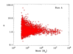
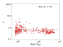
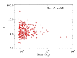
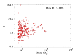
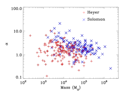
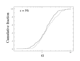
Figure 1: The distribution of the virial parameter ($\alpha$) is plotted with mass for clouds identified in Run A (top left, with magnetic fields), in the calculations with feedback adopting efficiencies of 1, 5 and 10 %, and the Heyer et al. (2009) data (lower middle). We find a population of predominantly unbound clouds, in rough agreement with the observations, for the models where localised gravitational collapse is limited by magnetic fields (Run A), or gravitational collapse occurs but there is a realistic level of stellar feedback (Run C, top right, Run D, lower left). There are many more bound clouds for the case with a very low level of stellar feedback (Run B, top middle). In the final panel (lower right), the cumulative fraction of clouds with a given $\alpha$ is shown for the Heyer data (dotted) and for the clouds from Run C, with 5 per cent efficiency (solid line). The KS test confirms that the distributions of $\alpha$ from the observations and simulations match, giving $P=0.11$ and $P=0.21$ for Runs C and D respectively.

2.1 Locating clouds

We identify clouds using the same method as described in Dobbs (2008). We apply a clumpfinding algorithm, which simply divides the simulation into a grid, and locates cells over a given surface density. Adjacent cells which exceed this criterion are grouped together and labelled as a cloud. Clouds which contain less than 30 particles are discarded, thus clouds in Runs B, C and D are at least $7.5\times 10^{4}$ M_⊙ (and clouds in Run A $3.75\times 10^{4}$ M_⊙). The mean number of particles in a cloud is $\sim 85$ for Runs A, B and C. The properties of the clumps reflect the total, rather than the molecular gas, but we would typically expect these clumps to exhibit high molecular fractions. For most of the results we present, we chose a surface density criterion of 100 M_⊙pc${}^{-2}\sim 4\times 10^{22}$ cm^-3. Changing this criterion has little effect on the distribution of the virial parameter, it merely reduces or increases the number of clouds selected.

For Runs C and D ($\epsilon=5$, 10 per cent), we are able to run the simulation for sufficiently long (300 Myr) that we can calculate cloud properties when the system has roughly reached equilibrium. However for Runs A (high surface density, no feedback) and B (1 % efficiency) we are limited by the high surface densities reached by a large fraction of the gas.

To illustrate the global structure of the disc in our models, the column density of the gas in Run C ($\epsilon=5$ per cent) is shown at a time of 200 Myr in Fig. 2. The dense gas is arranged into clouds along the spiral arms and spurs extending from the arm to interarm regions.

2.2 Virial parameter

In determining the virial parameters for our clouds, we calculate $\alpha$ as shown in Eqn. 1, where $\sigma_{v}$ is the line of sight velocity dispersion and $R$ is defined as the radius of a circle with the equivalent area of the cloud. This corresponds to that used by Heyer et al. (2009). We take bound clouds as having $\alpha<1$.

In the case with magnetic fields (Run A), we find largely unbound clouds, where local gravitational collapse is prevented by magnetic pressure. With minimal stellar feedback (Run B, $\epsilon=1$ per cent), we obtain many more bound clouds, particularly at higher masses. This clearly disagrees with the observations. For both Runs C and D ($\epsilon=5$ and 10 % respectively), we find that the clouds are predominantly unbound, and the distributions in the virial parameter, $\alpha$ are in agreement with the observations. This can be seen visually and is confirmed by comparing the distributions of $\alpha$ using the KS test (see also Fig. 1). Given the uncertainties in determining $\alpha$, if we require $\alpha>2$ for an unbound cloud, about half of the clouds in Runs C and D are unbound. There is little change in the fraction of unbound clouds with mass (and therefore resolution) in these calculations, with the exception of Run D, where feedback is responsible for preventing bound, higher mass clouds.

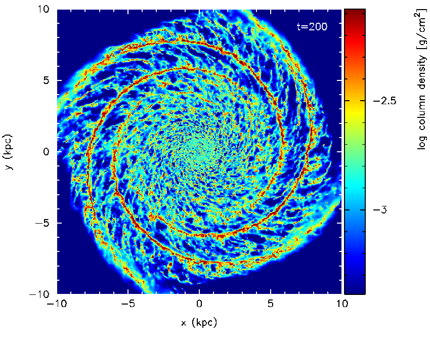
Figure 2: The gas column density is shown for Run C ($\epsilon=5$ per cent) at a time of 200 Myr. Dense gas, corresponding to the clouds located in the analysis presented here, predominantly lies along the arms, and spurs which extend from the arms into interarm regions.

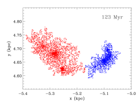
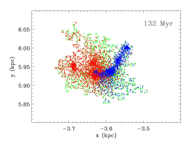
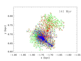
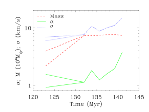
Figure 3: The evolution of a cloud from Run A is shown at times of 123 (top), 132 (second) and 141 (third panel) Myr. The evolution of the mass (in units of $10^{6}$ M_⊙), velocity dispersion and virial parameter are shown on the lowest panel. The two clouds in the top panel merge, and there is a subsequent increase in both the velocity dispersion and $\alpha$. They form a single clump of mass $7\times 10^{5}$ M_⊙. The initial clumps are coloured blue and red, so the constituent particles can be traced at later times. The particles coloured green are particles present in the clouds at 132 and 141 Myr, which were not present in the clumps at 123 Myr.

2.3 Evolution of individual clouds

The evolution of an individual cloud is often very complex, involving collisions, fragmentation and dispersion by feedback. Moreover the gas which constitutes a cloud can change on relatively short timescales. Thus studying the evolution of individual clouds, and establishing why they never, or rarely become gravitationally bound is not straightforward. In this Section we illustrate this behaviour by studying the nature and development of individual GMCs in the different calculations.

2.3.1 Cloud development in Run A

In Fig. 3, we highlight the contribution of collisions to the internal velocity dispersions of clouds in Run A. We show a collision between two clouds in Run A (which includes magnetic fields), where small scale gravitational collapse does not occur. After the collision between the two clouds, the velocity dispersion increases, which means the virial parameter also increases. The increase in the velocity dispersion is prolonged because the clouds contain substantial substructure – the merging of this substructure is seen in the middle panel. Thus the collisions between clouds are not really dissipative (as stated in Dobbs et al. (2006)); rather the energy is transferred to the internal motions of the clouds. We also simulated the cloud interaction shown in Fig. 3 in isolation, and at higher resolution, without magnetic fields or feedback. This confirmed that the collision induces random large scale motions which prevent widespread collapse in the cloud for around 10 Myr, independent of the magnetic field. This demonstrates that the energy input from cloud-cloud collisions can be comparable to, or even exceed the energy dissipated, i.e. a collision can lead to an increase in the global virial parameter. The generation of random velocities is analogous to that presented in previous work (Bonnell et al., 2006; Dobbs & Bonnell, 2007), and relies on the assumption that the ISM is clumpy on all scales.

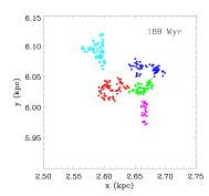
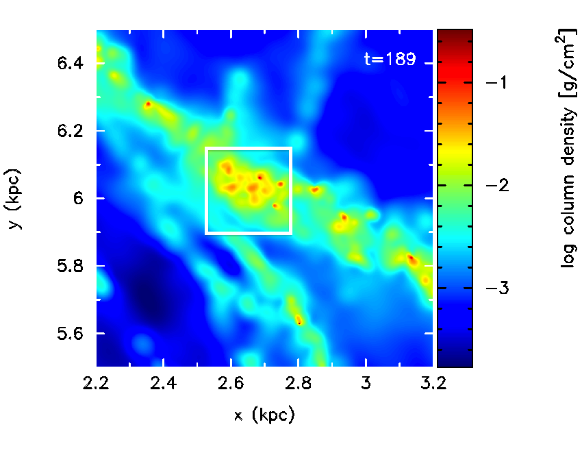
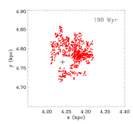
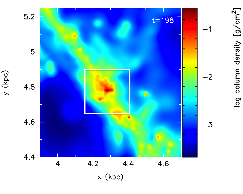
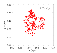
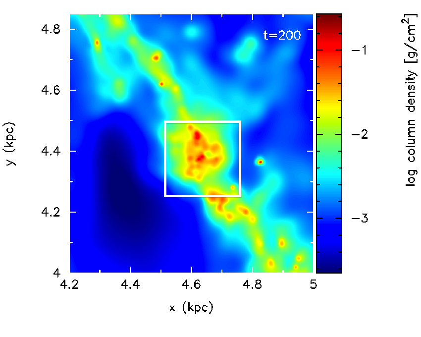
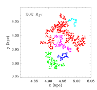
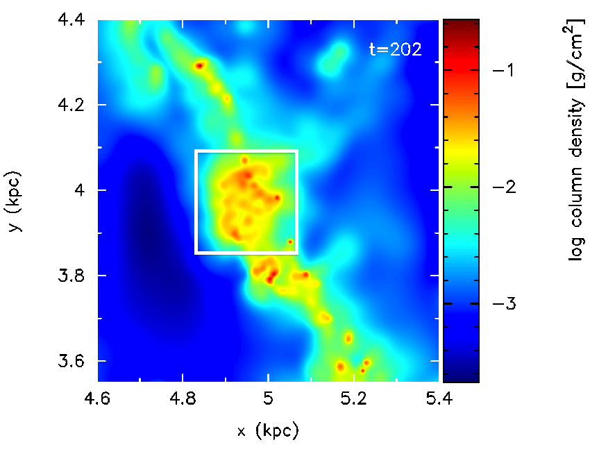
Figure 4: The evolution of a cloud from Run C (with 5 % efficiency stellar feedback) is shown, at 189 (top), 198 (second), 200 (third) and 202 (fourth panel) Myr. The cloud is formed by the merger of smaller clumps. Stellar feedback events (for example the cross in the second panel) then alter the shape of the cloud and finally result in the separation of the cloud into several separate clumps. Separate clumps, (as picked out by the clumpfinding algorithm), are shown simply in different colours, but the constituent particles are not all the same at different times. For example only 2/3 of the particles in the cloud at 198 Myr are in the cloud shown at 200 Myr. The right hand panels show column density images of the clumps and their surroundings. The white boxes indicate the size of the regions shown on the left hand panels. Fig. 5 shows the evolution of $\alpha$, the mass and the velocity disperions, $\sigma$, of the cloud, and the constituent clumps which formed the cloud.

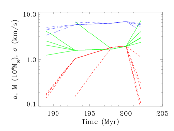
Figure 5: The evolution of $\alpha$ (green, solid), mass (red, dashed in units of $10^{6}$ M_⊙) and $\sigma$ (blue, dotted) of the clouds shown in Fig. 4. Cloud-cloud interactions have some role in determining the dynamics of the cloud, and maintaining $\sigma$, but $\sigma$ is dominated by stellar feedback. The different lines at 189 Myr (and the line at 193 Myr) correspond to several clumps merging to form one large cloud (193 Myr to 200 Myr). After 200 Myr, the cloud again splits up into multiple components, due to feedback.

2.3.2 Run C: a multiple cloud interaction with feedback

In Fig. 4 we show the evolution and interaction of a multiple set of clouds in Run C ($\epsilon=$5 per cent). A single cloud was selected at a time of 198 Myr, and the clouds which contain the same particles were identified at earlier and later times. We find that the cloud identified at 198 Myr is formed from the mergers of several smaller clouds. In the first panel (189 Myr) we can identify 5 separate clouds. As these merge to produce a cloud of $2\times 10^{6}$ M_⊙ some 9 Myr later, the effects of stellar feedback can be seen for example in the cloud in the second panel (a bubble blown out by feedback is indicated by the cross). Feedback plays a large role in shaping the cloud, and regulating the dynamics. The clouds, as picked out by the clumpfinding algorithm (left hand plots) show much more filamentary structures compared to the clouds in Run A (Fig. 3). By 202 Myr (4th panel), stellar feedback has succeeded blowing away the top part of the cloud, and splitting the cloud apart. Over the course of the plots shown (13 Myr), there are 5 supernovae events in the cloud. In Fig. 5 we show the corresponding evolution of $\alpha$ and the velocity dispersion. It can be seen that the velocity dispersion is maintained at about 6 km s^-1, and the virial parameter, $\alpha$, above unity throughout. Thus in this case, a multiple cloud collision together with feedback (from small regions of the cloud which become bound and allow star formation) maintains the unbound nature of the cloud as a whole.

It can also be seen from Fig. 4 (right hand panels) that the clouds we identify are part of a larger region of dense gas, which is hundreds as opposed to tens of parsecs in size. In a galaxy with a high molecular gas fraction such a feature would correspond to a Giant Molecular Association (GMA). Whilst these regions are still unbound in our calculations, they appear to have a longer lifetime than the GMC sized clouds.

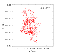
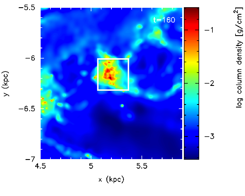
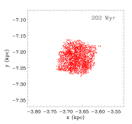
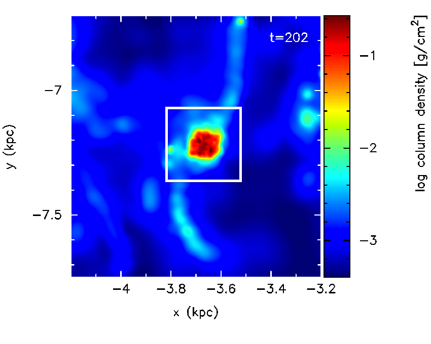
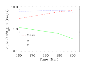
Figure 6: The evolution of a second cloud from Run C, with 5 % efficiency stellar feedback. Unlike the cloud shown in Fig. 4, this cloud is too massive to be disrupted by feedback or collisions and becomes increasingly more massive, and bound with time. At 160 Myr (top panel), the cloud is still filamentary, and marginally unbound. By 200 Myr (lower panel), the cloud contains no filamentary structure and is strongly bound. The right hand panels show column density images of the regions containing the clouds on the left, the white boxes indicating the sizes of the left hand plots. The lowest panel shows the evolution of $\alpha$, mass (in units of $10^{6}$ M_⊙) and $\sigma$ for the cloud.

2.3.3 Run C: the evolution of an isolated massive cloud

For the calculation, with 5 % efficiency feedback (Run C), the timescales for the majority of clouds to merge and become disrupted are relatively short, of order several Myr. The exceptions are two longlived bound clouds, which have masses of $3\times 10^{6}$ M_⊙ and $5\times 10^{6}$ M_⊙ respectively. These are the high mass points seen in Fig. 1 (top right plot). We show the evolution of the $5\times 10^{6}$ M_⊙ cloud in Fig. 6 over a period of 40 Myr. The top panel shows the cloud at a time of 160 Myr, when the cloud is clearly irregular in shape. By 200 Myr, the cloud has a much more regular, quasi-spherical appearance and is not filamentary in any way. This cloud finds itself in between the spiral arms, and does not undergo any significant interactions with other clouds after 160 Myr. In the lower panel, we plot the evolution of $\alpha$, the velocity dispersion and the mass. We see that the cloud is continuing to accrete material, and grow in mass, becoming steadily more bound. Feedback (with $\epsilon=$5 per cent) is insufficient to disrupt the cloud, although feedback does maintain a constant velocity dispersion of $\sim$6 km s^-1. It is likely that this cloud would eventually form a bound stellar cluster, though we do not attempt to follow this in our calculation. In Run B ($\epsilon=1$ per cent) there are many more clouds which display this behaviour.

2.4 The constituent gas of the clouds

In the current paradigm of molecular cloud formation and evolution, GMCs are assumed to be bound objects which consist of essentially the same gas for the duration of their lifetimes. In Fig. 7 we take all the clouds at a given time in Run C ($\epsilon=5$ per cent), and plot the percentage of gas which remains in a given cloud after 10 Myr.

In all cases we find that the constituent gas of the clouds changes on timescales of $<10$ Myr. We find that about 50 per cent of clouds are completely dispersed within 10 Myr. A substantial fraction of clouds are shortlived, either dispersing to lower densities, merging with other clouds to produce more massive clouds, or some combination of these processes. There are a few clouds which substantially retain their identity over a period of $>$10 Myr.

This highlights that generally the constituent gas in GMCs is likely to change on timescales of Myr. This may mean that discussing clouds lifetimes, which are thought to be 20-30 Myr (Leisawitz et al., 1989; Kawamura et al., 2009), may not make sense. A cloud seen after 30 Myr may not be a counterpart to any cloud present at the current time. In our calculations this is only true for the most massive clouds.

Thus we see that the clouds tend to display a variety of behaviours. The relatively low mass GMCs undergo frequent collisions, are readily disrupted, and $\alpha$ will change accordingly. Even if the cloud becomes bound, it may undergo another dynamical interaction on a short timescale, and become unbound. In contrast the more massive clouds undergo less dramatic behaviour. There are relatively few clouds of this mass, so they very rarely undergo collisions with objects of a similar size, whilst above a certain mass they are not so easily torn apart by feedback.

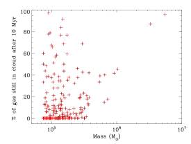
Figure 7: The percentage of gas which still lies in the same cloud after 10 Myr is plotted versus the cloud’s mass for clouds identified in Run C (with stellar feedback and $\epsilon=5$ per cent). This percentage is calculated by locating clouds at 2 timeframes, 10 Myr apart. We search for the constituent gas particles of a given cloud in the clouds present 10 Myr later. Sometimes there may be more than one cloud containing the particles of an earlier cloud (and in some instances no clouds!), in which case we select the cloud which has the maximum of the particles the same as the cloud at the earlier time frame. In 35 per cent of cases the clouds are completely disrupted, whilst the median amount of gas remaining in the cloud is 22 per cent.

2.5 The shapes of clouds

From our calculations with different levels of feedback, we obtain distributions of clouds which are predominantly unbound (Runs C and D, with 5 and 10 % efficiency) or bound (Run B, with 1 % efficiency). We have demonstrated that the observations are most likely fit by a distribution of mainly unbound clouds.

In addition, we find that, the bound clouds are much more regular, spherically shaped, whilst the unbound clouds have very irregular shapes. Koda et al. (2006) carried out a study of Galactic molecular clouds and determined the aspect ratios of the clouds. Their results are shown in Fig. 8, and indicate the most common aspect ratios are between 1.5 and 2. We also show in Fig. 8 the distributions of aspect ratios for the calculations with low feedback Run B (predominantly bound clouds), and the higher feedback case, Run C (predominantly unbound clouds).

In Run C (centre panel), with feedback efficiency of 5 per cent, the distribution of aspect ratios has reached an equilibrium state, and is found to be similar to observations, with a peak at about 1.5. In Run B (left panel), with 1 % efficiency, equilibrium has yet to be achieved, and more and more clouds have aspect ratios of around unity with increasing time. As we would expect, the virialised clouds tend to have aspect ratios close to unity. The prominent peak at aspect ratios of unity does not agree with the observations, reconfirming our previous conclusions that the simulations with efficiencies of 5 – 10 per cent are in best agreement with the observations.

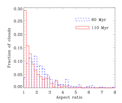
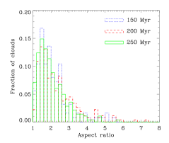
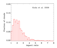
Figure 8: The distribution of aspects ratios of the clouds is shown for the models with 1 % efficiency feedback (Run B, left), and 5 % efficiency feedback (Run C, centre). The distribution of aspect ratios for Galactic clouds is shown on the right (Koda et al., 2006). The clouds for the 5 % efficiency case (centre) reasonably match the observations,although even in this case our clouds are slightly more peaked towards low aspect ratios than the observations. The distribution does not change with time, once equilibrium has been established. With 1 % efficiency (left), the distribution evolves to a strong peak at 1, in definite contradiction to the observations.

3 Discussion

In this paper we have addressed the recent observational evidence that most molecular clouds within the Galaxy are not gravitationally bound. This evidence contrasts with the original claims of Solomon et al. (1987), long since propagated into the field, that molecular clouds are bound and in virial equilibrium. The idea that molecular clouds are bound entities has also been taken as a starting point for many theories of star formation.

Of course, for star formation to take place it is necessary that some parts of a cloud be self-gravitating and able to undergo collapse. What the observations seem to indicate however is that it is not necessary for the cloud as a whole to be dominated by gravity. With this in mind, we present here simulations of the ISM in a galaxy with a fixed spiral potential. By including simple heating and cooling of the gas, we are able to identify those parts of the ISM which are dense enough to represent molecular gas, and so are able to identify what would be observed as molecular clouds. We allow the parts of those clouds which are sufficiently dense and sufficiently gravitationally bound to notionally form stars. Because such clouds are generally highly inhomogeneous entities, within them there will be some regions (in our simulations typically representing only $<30$ percent of the mass) which are gravitationally bound, and within which star formation takes place. This star formation is taken to manifest itself as an input of energy and momentum into the surrounding gas. The global galactic star formation rate is in accordance with the results of Kennicutt (1998).

Using this simple, and highly idealised, input physics we are able to reproduce both the observed distribution of virial parameters of molecular clouds in the Galaxy (with most of the clouds being unbound) and also the observed distribution of cloud shapes (in terms of their aspect ratios). We find that the velocity dispersions within clouds are maintained not just by feedback from star formation but also by collisions between non-homogeneous clouds (cf. Dobbs & Bonnell 2007). However with no, or little feedback, the clouds are predominantly bound and quasi-spherical (as found in Run B and by Tasker & Tan 2009), in disagreement with observations.

We also find that the constituent material of a typical cloud only remains within that cloud for a timescale of around 10 Myr. Thus for timescale much longer than this, the concept of a cloud lifetime is no longer meaningful.

We note that the properties and lifetimes of clouds depend somewhat on the size scales considered. Above some surface density threshold, we would expect to start selecting bound regions within a GMC, and therefore we would obtain a higher fraction of bound objects. We have not considered the properties of larger GMAs either. The fraction of unbound clouds also depends on how we define $\alpha$, and what threshold we use. However we note that for our clouds, even if $\alpha$ is low, external energy input from collisions, and feedback sources within a cloud can act to increase $\sigma_{v}$, and therefore $\alpha$. Thus the main difference between our models and previous analaysis, for example that presented by Ballesteros-Paredes et al. (2010), is that collisions and feedback play a much more important role.

In summary, the idea that all molecular clouds are gravitationally bound entities is neither observationally viable, nor theoretically necessary. It is no real surprise that most molecular clouds identified in the Galaxy are globally unbound, and that the rest are at most only marginally bound.

4 Acknowledgments

We thank a number of people who read through a draft of this paper, provided many helpful comments and highlighted issues which required clarity: Rob Kennicutt, Lee Hartmann, Mark Heyer, Bruce Elmegreen, Fabian Heitsch, Javier Ballesteros-Paredes. We thank Ralf Klessen for providing a useful referee’s report. CLD also thanks Jin Koda for providing the data for Figure 8, right panel, and Ian Bonnell for helpful discussions. The research of A.B. is supported by a Max Planck Fellowship and by the DFG Cluster of Excellence “Origin and Structure of the Universe”. The calculations presented in this paper were primarily performed on the HLRB-II: SGI Altix 4700 supercomputer and Linux cluster at the Leibniz supercomputer centre, Garching. Run A was performed on the University of Exeter’s SGI Altix ICE 8200 supercomputer. Some of the figures in this paper were produced using SPLASH (Price, 2007), a visualization tool for SPH that is publicly available at http://www.astro.ex.ac.uk/people/dprice/splash.

References

- Allen & Shu (2000) Allen A., Shu F. H., 2000, ApJ, 536, 368
- Ballesteros-Paredes (2006) Ballesteros-Paredes J., 2006, MNRAS, 372, 443
- Ballesteros-Paredes et al. (2010) Ballesteros-Paredes J., Hartmann L. W., Vázquez-Semadeni E., Heitsch F., Zamora-Avilés M. A., 2010, ArXiv e-prints
- Ballesteros-Paredes et al. (2007) Ballesteros-Paredes J., Klessen R. S., Mac Low M., Vazquez-Semadeni E., 2007, Protostars and Planets V, pp 63–80
- Basu & Mouschovias (1994) Basu S., Mouschovias T. C., 1994, ApJ, 432, 720
- Bate et al. (1995) Bate M. R., Bonnell I. A., Price N. M., 1995, MNRAS, 277, 362
- Benz et al. (1990) Benz W., Cameron A. G. W., Press W. H., Bowers R. L., 1990, ApJ, 348, 647
- Bertoldi & McKee (1992) Bertoldi F., McKee C. F., 1992, ApJ, 395, 140
- Binney & Tremaine (1987) Binney J., Tremaine S., 1987, Galactic dynamics. Princeton, NJ, Princeton University Press, 1987, 747 p.
- Bolatto et al. (2008) Bolatto A. D., Leroy A. K., Rosolowsky E., Walter F., Blitz L., 2008, ApJ, 686, 948
- Bonnell et al. (2006) Bonnell I. A., Dobbs C. L., Robitaille T. R., Pringle J. E., 2006, MNRAS, 365, 37
- Bonnell et al. (2010) Bonnell I. A., Smith R. J., Clark P. C., Bate M. R., 2010, ArXiv e-prints
- Caldwell & Ostriker (1981) Caldwell J. A. R., Ostriker J. P., 1981, ApJ, 251, 61
- Clark et al. (2008) Clark P. C., Bonnell I. A., Klessen R. S., 2008, MNRAS, 386, 3
- Clark et al. (2005) Clark P. C., Bonnell I. A., Zinnecker H., Bate M. R., 2005, MNRAS, 359, 809
- Cox & Gómez (2002) Cox D. P., Gómez G. C., 2002, ApJS, 142, 261
- Dib et al. (2007) Dib S., Kim J., Vázquez-Semadeni E., Burkert A., Shadmehri M., 2007, ApJ, 661, 262
- Dobbs (2008) Dobbs C. L., 2008, MNRAS, 391, 844
- Dobbs & Bonnell (2007) Dobbs C. L., Bonnell I. A., 2007, MNRAS, 374, 1115
- Dobbs et al. (2006) Dobbs C. L., Bonnell I. A., Pringle J. E., 2006, MNRAS, 371, 1663
- Dobbs et al. (2008) Dobbs C. L., Glover S. C. O., Clark P. C., Klessen R. S., 2008, MNRAS, 389, 1097
- Dobbs & Price (2008) Dobbs C. L., Price D. J., 2008, MNRAS, 383, 497
- Elmegreen (2002) Elmegreen B. G., 2002, ApJ, 577, 206
- Elmegreen (2007) Elmegreen B. G., 2007, ApJ, 668, 1064
- Glover et al. (2010) Glover S. C. O., Federrath C., Mac Low M., Klessen R. S., 2010, MNRAS, 404, 2
- Hartmann et al. (2001) Hartmann L., Ballesteros-Paredes J., Bergin E. A., 2001, ApJ, 562, 852
- Heitsch et al. (2001) Heitsch F., Mac Low M., Klessen R. S., 2001, ApJ, 547, 280
- Heyer et al. (2009) Heyer M., Krawczyk C., Duval J., Jackson J. M., 2009, ApJ, 699, 1092
- Heyer et al. (2001) Heyer M. H., Carpenter J. M., Snell R. L., 2001, ApJ, 551, 852
- Kawamura et al. (2009) Kawamura A., Mizuno Y., Minamidani T., Filipović M. D., Staveley-Smith L., Kim S., Mizuno N., Onishi T., Mizuno A., Fukui Y., 2009, ApJS, 184, 1
- Kennicutt (1998) Kennicutt R. C., 1998, ARA&A, 36, 189
- Klessen et al. (2000) Klessen R. S., Heitsch F., Mac Low M., 2000, ApJ, 535, 887
- Klessen & Hennebelle (2010) Klessen R. S., Hennebelle P., 2010, A&A, 520, A17+
- Koda et al. (2006) Koda J., Sawada T., Hasegawa T., Scoville N. Z., 2006, ApJ, 638, 191
- Krumholz et al. (2006) Krumholz M. R., Matzner C. D., McKee C. F., 2006, ApJ, 653, 361
- Krumholz & McKee (2005) Krumholz M. R., McKee C. F., 2005, ApJ, 630, 250
- Leisawitz et al. (1989) Leisawitz D., Bash F. N., Thaddeus P., 1989, ApJS, 70, 731
- Mac Low & Klessen (2004) Mac Low M.-M., Klessen R. S., 2004, Reviews of Modern Physics, 76, 125
- Monaghan (1997) Monaghan J. J., 1997, Journal of Computational Physics, 136, 298
- Mouschovias et al. (2006) Mouschovias T. C., Tassis K., Kunz M. W., 2006, ApJ, 646, 1043
- Price (2007) Price D. J., 2007, Publications of the Astronomical Society of Australia, 24, 159
- Price & Bate (2008) Price D. J., Bate M. R., 2008, MNRAS, 385, 1820
- Price & Monaghan (2007) Price D. J., Monaghan J. J., 2007, MNRAS, 374, 1347
- Pringle et al. (2001) Pringle J. E., Allen R. J., Lubow S. H., 2001, MNRAS, 327, 663
- Rosolowsky (2007) Rosolowsky E., 2007, ApJ, 654, 240
- Shetty et al. (2010) Shetty R., Collins D. C., Kauffmann J., Goodman A. A., Rosolowsky E. W., Norman M. L., 2010, ApJ, 712, 1049
- Shetty et al. (2010) Shetty R., Glover S. C., Dullemond C. P., Klessen R. S., 2010, ArXiv e-prints
- Shu et al. (1987) Shu F. H., Adams F. C., Lizano S., 1987, ARA&A, 25, 23
- Shu et al. (2007) Shu F. H., Allen R. J., Lizano S., Galli D., 2007, ApJL, 662, L75
- Solomon et al. (1987) Solomon P. M., Rivolo A. R., Barrett J., Yahil A., 1987, ApJ, 319, 730
- Tasker & Tan (2009) Tasker E. J., Tan J. C., 2009, ApJ, 700, 358
- Vázquez-Semadeni et al. (2005) Vázquez-Semadeni E., Kim J., Shadmehri M., Ballesteros-Paredes J., 2005, ApJ, 618, 344
- Wolfire et al. (2003) Wolfire M. G., McKee C. F., Hollenbach D., Tielens A. G. G. M., 2003, ApJ, 587, 278
- Zuckerman & Evans (1974) Zuckerman B., Evans II N. J., 1974, ApJL, 192, L149