Perspectives on double-excitations in TDDFT

Abstract

The adiabatic approximation in time-dependent density functional theory (TDDFT) yields reliable excitation spectra with great efficiency in many cases, but fundamentally fails for states of double-excitation character. We discuss how double-excitations are at the root of some of the most challenging problems for TDDFT today. We then present new results for (i) the calculation of autoionizing resonances in the helium atom, (ii) understanding the nature of the double excitations appearing in the quadratic response function, and (iii) retrieving double-excitations through a real-time semiclassical approach to correlation in a model quantum dot.

I Introduction

There is no question that time-dependent density functional theory (TDDFT) has greatly impacted calculations of excitations and spectra of a wide range of systems, from atoms and molecules, to biomolecules and solids TDDFTbook ; RG84 . Its successes have encouraged bold and exciting applications to study systems as complex as photosynthetic processes in biomolecules, coupled electron-ion dynamics after photoexcitation, molecular transport, e.g. Refs. TTRF08 ; KCBC08 ; EFB07 ; SRVB09 . The usual approximations used for the exchange-correlation (xc) potential in TDDFT calculations however perform poorly in a number of situations particularly relevant for some of these applications, e.g. states of double-excitation character MZCB04 , long-range charge-transfer excitations DWH03 ; T03 , conical intersections LKQM06 ; TTRF08 , polarizabilities of long-chain polymers FBLB02 , optical response in solids ORR02 ; GORT07 . Improved functionals, modeled from first-principles, have been developed, and are beginning to be used, to treat some of these. In this paper, we focus on the problem of double-excitations in TDDFT, for which recently much progress has been made.

The term “double-excitation” is a short-hand for “state of double-excitation character”. In a non-interacting picture, such as Kohn-Sham (KS), a double-excitation means one in which two electrons have been promoted out of orbitals occupied in the ground-state, to two virtual orbitals, forming a “doubly-excited” Slater determinant. The picture of placing electrons in single-particle orbitals however does not apply to true interacting states. Instead one may expand any interacting state as a linear combination of Slater determinants, say eigenstates of some one-body Hamiltonian, such as the KS Hamiltonian, and then a state of double-excitation character is one which has a significant proportion of a doubly-excited Slater determinant. Clearly, the exact value of this proportion depends on the level of theory used for the ground-state reference e.g. it will be different in Hartree-Fock than in TDDFT.

Given the important role of correlation in states of double-excitation character, the question of how these appear in a single-particle-based theory has both fundamental and practical interest. We shall begin by reviewing the status of linear-response TDDFT in this regard: one must go beyond the ubiquitous adiabatic approximation to capture these. We conclude the introduction by discussing systems where double-excitations are particularly important, and we shall see that some of these cases are due to the peculiarity of the KS single-Slater determinant in the ground-state (e.g. in certain long-range charge-transfer states). Then in Section II we consider what happens when the double-excitation lies in the continuum, and test a recently developed kernel approximation to describe the resulting autoionizing resonance in the He atom. In Section III, we study whether adiabatic kernels can be redeemed for double-excitations by going to quadratic response theory. Section IV turns to a new approach that was recently proposed for general many-electron dynamics, that uses semiclassical dynamics to evaluate electron correlation. Here we test it on a model system to see whether it captures double-excitations.

I.1 Double excitations in linear-response TDDFT

Excitation spectra can be obtained in two ways from TDDFT. In one, a weak perturbation is applied to the KS system in its ground-state, and the dynamics in real-time of, e.g. the dipole moment is Fourier transformed to reveal peaks at the excitation frequencies of the system, whose strengths indicate the oscillator strength. More often, a formulation directly in the frequency-domain is used, in which two steps are performed: First, the KS orbital energy differences between occupied ($i$) and unoccupied ($a$) orbitals, $\omega_{\scriptscriptstyle\rm S}=\epsilon_{a}-\epsilon_{i}$ are computed. Second, these frequencies are corrected towards the true excitations through solution of a generalized eigenvalue problem PGG96 ; C96 , utilizing the Hartree-exchange-correlation kernel, $f_{\scriptscriptstyle\rm HXC}[n_{0}]({\bf r},{\bf r}^{\prime},\omega)=1/|{\bf r}-{\bf r}^{\prime}|+f_{\scriptscriptstyle\rm XC}[n_{0}]({\bf r},{\bf r}^{\prime},\omega)$, a functional of the ground-state density $n_{0}({\bf r})$.

Fundamentally, the origin of the linear response formalism is the Dyson-like equation that links the density-density response function of the non-interacting KS system, $\chi_{\scriptscriptstyle\rm S}$, with that of the true system, $\chi$:

$$\chi(\omega)=\chi_{\scriptscriptstyle\rm S}(\omega)+\chi_{\scriptscriptstyle\rm S}(\omega)\star f_{\scriptscriptstyle\rm HXC}(\omega)\star\chi(\omega)$$ (1)

where we use the shorthand $\star$ to indicate the integral, $\chi_{\scriptscriptstyle\rm S}(\omega)\star f_{\scriptscriptstyle\rm HXC}(\omega)=\int d^{3}r_{1}\ \chi_{\scriptscriptstyle\rm S}({\bf r},{\bf r}_{1},\omega)f_{\scriptscriptstyle\rm HXC}({\bf r}_{1},{\bf r}^{\prime},\omega)$ thinking of $\chi,\chi_{\scriptscriptstyle\rm S},f_{\scriptscriptstyle\rm HXC}$ etc as infinite-dimensional matrices in ${\bf r},{\bf r}^{\prime}$, each element of which is a function of $\omega$. The interacting density-density response function $\chi[n_{0}]({\bf r},{\bf r}^{\prime},t-t^{\prime})=\delta n({\bf r},t)/\delta v({\bf r}^{\prime}t^{\prime})|_{n=n_{0}}$ measures the response in the density $n({\bf r},t)$ to a perturbing external potential $v({\bf r},t)$. In the frequency domain,

$$\chi({\bf r},{\bf r}^{\prime},\omega) = \sum_{I}\left(\frac{\langle\Psi_{0}|\hat{n}({\bf r})|\Psi_{I}\rangle\langle\Psi_{I}|\hat{n}({\bf r}^{\prime})|\Psi_{0}\rangle}{\omega-\omega_{I}+i0^{+}}\right.$$ (2)

$$- \left.\frac{\langle\Psi_{0}|\hat{n}({\bf r}^{\prime})|\Psi_{I}\rangle\langle\Psi_{I}|\hat{n}({\bf r})|\Psi_{0}\rangle}{\omega+\omega_{I}+i0^{+}}\right)$$

where $I$ labels the interacting excited-states, and $\omega_{I}=E_{I}-E_{0}$ is their frequency relative to the ground-state. Similar expressions hold for the KS system, substituting the interacting wavefunctions above with KS single-Slater-determinants.

In almost all calculations, an adiabatic approximation is made for the exchange-correlation (xc) kernel, i.e. one that is frequency-independent, corresponding to an xc potential that depends instantaneously on the density. But it is known that the exact kernel is non-local in time, reflecting the xc potential’s dependence on the history of the density. It is perhaps surprising that the adiabatic approximation works as well as it does, given that even weak excitations of a system lead it out of a ground-state (even if its density is that of a ground-state). One of the reasons for its success for general excitation spectra is that the KS excitations themselves are often themselves good zeroth-order approximations. But this reason cannot apply to double-excitations, since double-excitations are absent in linear response of the KS system: to excite two electrons of a non-interacting system two photons would be required, beyond linear response. Only single-excitations of the KS system are available for an adiabatic kernel to mix. Indeed, if we consider the KS linear density response function, the numerator of Eq. 2 with KS wavefunctions contains $\langle\Phi_{0}|\hat{n}({\bf r})|\Phi_{I}\rangle$, which vanishes if the excited determinant $\Phi_{I}$ differs from the ground-state $\Phi_{0}$ by more than one orbital. The one-body operator $\hat{n}({\bf r})$ cannot connect states that differ by more than one orbital. The true response function, on the other hand, retains poles at the true excitations which are mixtures of single, double, and higher-electron-number excitations, as the numerator $\langle\Psi_{0}|\hat{n}({\bf r})|\Psi_{I}\rangle$ remains finite due to the mixed nature of both $\Psi_{0}$ and $\Psi_{I}$. Within the adiabatic approximation, $\chi$ therefore contains more poles than $\chi_{\scriptscriptstyle\rm S}$.

Ref. TH00 pointed out the need to go beyond the adiabatic approximation in capturing states of double-excitation character. Ref. MZCB04 derived a frequency-dependent kernel, motivated by first-principles, to be applied within the subspace of single KS excitations that mix strongly with the double-excitation of interest. For the case of one single-excitation, $q=i\to a$, coupled to one double-excitation:

$$2[q|f_{\scriptscriptstyle\rm XC}(\omega)|q]=2[q|f_{\scriptscriptstyle\rm XC}^{A}(\omega_{q})|q]+\frac{|H_{qD}|^{2}}{\omega-(H_{DD}-H_{00})}.$$ (3)

to be applied within a dressed single-pole approximation (“DSPA”),

$$\omega=\omega_{q}+2[q|f_{\scriptscriptstyle\rm XC}(\omega)|q]$$ (4)

The Hamiltonian matrix elements in the dynamical correction (second term of Eq. (3)) are those of the true interacting Hamiltonian, taken between the single ($q$) and double ($D$) KS Slater determinants of interest, as indicated, and $H_{00}$ is the expectation value of the true Hamiltonian in the KS ground-state. This can be generalized to cases where several single-excitations and double-excitations strongly mix, within a “dressed Tamm-Dancoff” scheme (see, e.g. CZMB04 ; MW09 ). The kernel is to be applied as an a posteriori correction to a usual adiabatic calculation: first, one scans over the KS orbital energies to see if the sum of two of their frequencies lies near a single excitation frequency, and then applies this kernel just to that pair.

Essentially the same formula results from derivations with different starting points: in Ref. C05 , it emerges as a polarization propagator correction to adiabatic TDDFT in a superoperator formalism, made more rigorous in Ref. HC10a . Ref. RSBS09 utilized the Bethe-Salpeter equation with a dynamically screened Coulomb interaction. while Ref. GB09 extended the original approach of Ref. MZCB04 by taking account of the coupling of the single-double pair with the entire KS spectrum via the common energy denominator approximation (CEDA).

I.2 When are double excitations important?

Even the low-lying spectra of some molecules are interspersed with states of double-excitation character, but we will argue that they also lie at the root of several significant challenges approximate TDDFT faces for spectra and photo-dynamics. Although not traditionally seen as a double-excitation problem, we will see that double-excitations haunt the difficulty in describing conical intersections and certain long-range charge-transfer states.

Molecular spectra First, double-excitations in their own right are prominent in the low-lying spectra of many conjugated polymers. A famous case is the class of polyenes (see Ref.CZMB04 for many references). For example, in butadiene the HOMO to (LUMO+1) and (HOMO-1) to LUMO excitations are near-degenerate with a double-excitation of the HOMO to LUMO. If one runs an adiabatic calculation and simply assigns the energies according to an expected ordering, one obtains 7.02eV for the vertical excitation from a B3LYP calculation (similar with other hybrid functionals), in a 6-311G(d,p) basis set, while a CASPT2 calculation yields 6.27eV. By using different basis sets, a more accurate value can appear, but rather fortuitously, since the state obtained in adiabatic B3LYP has more of a Rydberg character, rather than double character HHH01 . In Ref. CZMB04 , the dressing Eq. (3), generalized to a subspace of two KS single excitations instead of one, was applied, yielding 6.28eV. Similar successes were computed for hexatriene, and also for 0-0 excitations. This system was later studied in detail in Ref. MW09 , analyzing more fully aspects such as self-consistent treatment of the kernel, and use of KS versus Hartree-Fock orbitals in the dressing. Further, in Ref. MMWA11 , excited state geometries were successfully computed in this way. Most recently, an extensive study of Eq. (3) was performed in Ref. HIRC10 to low-lying states of 28 organic molecules.

Charge-transfer excitations It is well known that long-range charge-transfer excitations are severely underestimated with the usual approximations of TDDFT. The usual argument to explain this is that the TDDFT correction to the bare KS orbital energy difference vanishes because the occupied and unoccupied orbitals, one being located on the donor and the other on the acceptor, have negligible overlap as the donor-acceptor distance increases DWH03 ; T03 ; A09 . The TDDFT prediction then reduces to the bare KS orbital energy difference, $\epsilon_{L}({\rm acceptor})-\epsilon_{H}({\rm donor})$ where the subscripts $H$ and $L$ refer to HOMO and LUMO, respectively. This typically leads to an underestimation, because in usual approximations $|\epsilon_{H}|$ underestimates the true ionization energy, while the lowest unoccupied molecular orbital (LUMO), $\epsilon_{\rm L}$, lacks relaxation contributions to the electron affinity. The last few years have seen many methods to correct the underestimation of CT excitations, e.g. Refs. TTYY04p ; SKB09 ; HIG09 ; most modify the ground-state functional to correct the approximate KS HOMO’s underestimation of $I$, and mix in some degree of Hartree-Fock, and most, but not all SKB09 ; HIG09 determine this mixing via at least one empirical parameter.

But the argument above only applies to the case where the donor and acceptor are closed-shell species; instead, if we are interested in charge-transfer between open-shell species (e.g. in something like LiH), the HOMO and LUMO are delocalized over the whole molecule. This is the case for the exact ground-state KS potential, as well as for semi-local approximations TMM09 . The exact KS potential has a peak and a step in the bonding region, that has exactly the size to realign the atomic HOMO’s of the two fragments P85b ; PPLB82 ; TMM09 (see also Fig. 1). As a result the molecular HOMO and LUMO are delocalized over the whole molecule. The HOMO-LUMO energy difference goes as the tunnel splitting between the two fragments, vanishing as the molecule is pulled apart; therefore every excitation out of the KS HOMO is near-degenerate with a double-excitation where a second electron goes from the HOMO to the LUMO (at almost zero KS cost). This KS double-excitation is crucial to capture the correct nature of the true excitations as otherwise we are left with half-electrons on each fragment, physically impossible in the dissociated limit. This strongly affects the kernel structure, imposing a severe frequency-dependence for all excitations, charge-transfer and local, for heteroatomic molecules composed of open-shell fragments at large separation M05c ; MT06 .

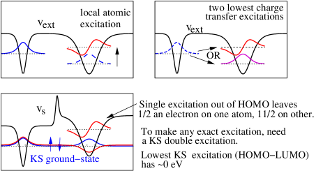
Figure 1: Excitations out of a heteroatomic molecule composed of open-shell fragments at long-range (eg. ”stretched” LiH). Blue denotes orbitals occupied in the ground-state; in this model, we show one electron on each ”atom” (the inner electrons play only a secondary role). The top panel shows a model of the possible excitations of the true system: on the left is a local excitation on one atom, on the right are shown two lowest charge-transfer excitations. The bottom left panel shows the corresponding KS potential, displaying a step and a peak, as discussed in the text. The ground-state KS is the doubly-occupied bonding orbital; any single excitation out of here is near-degenerate with a double-excitation where the other electron occupying the bonding orbital transits to the near-degenerate antibonding LUMO.

Coupled electron-nuclear dynamics The importance of double-excitations for coupled electron-nuclear dynamics was highlighted in Ref. LKQM06 : even when the vertical excitation does not contain much double-excitation character, the propensity for curve-crossing requires accurate double-excitation description for accurate global potential energy surfaces. The same paper pointed out the difficulties TDDFT has with obtaining conical intersections: in one example there, the TDDFT dramatically exaggerated the shape of the conical intersection, while in another, its dimensionality was wrong, producing a seam rather than a point. Although a primary task is to correct the ground-state surface, the problem of double-excitations is likely very relevant around the conical intersections due to the near-degeneracy.

Autoionizing resonances In the next section we discuss the case when the excitation energy of a double-excitation is larger than the ionization energy of the system. In this case, an autoionizing resonance results.

II Autoionizing Resonances in the He atom

Photoionization has a rich history in quantum mechanics, with the photoelectric effect playing a pivotal role in establishing the dual nature of light, and continues to be a valuable tool in analyzing atoms, molecules, and solids. The photospectra above the ionization threshold are characterized by autoionizing resonances, whereby bound state excitations interact with those into the continuum. Many theoretical methodsF78 ; KG88 ; SM08 ; SC01 ; LL00 ; CMR00 have been developed in order to predict these resonances.

As TDDFT is both accurate and relatively computationally inexpensive, it stands as a useful candidate for studying these excitations. For autoionizing resonances where a single excitation frequency (e.g. core $\rightarrow$ Rydberg) lies in the continuum, TDDFT has been shown to work wellSFD05 ; FSD03 ; FSD04 ; STFD06 ; STFD07 ; SDL95 ; HB09 . However it was notedSDL95 ; FSD04 that resonances arising from bound double excitations are completely missing in the adiabatic approximation (as we might expect from section I.2).

Ref. KM09, derived a frequency-dependent kernel which allows TDDFT to predict bound-double autoionizing resonances. Below we review this derivation before testing it on the Helium atom.

II.1 Frequency-dependent kernel for autoionizing double-excitations

Fano’s pioneering work on photoionization F61 considered a zeroth-order unperturbed system with a bound state $\Phi_{b}$ degenerate with that of a continuum state $\Phi_{E}$. The unperturbed system differs from the true system by the coupling term $\hat{V}_{cpl}$, and we define the matrix element $V_{E}=\langle\Phi_{E}|\hat{V}_{cpl}|\Phi_{b}\rangle$ between the two states. The transition probability, for some transition operator $\hat{T}$ (e.g. the dipole), between an initial state $|i\rangle$ and the mixed state with energy in the continuum was then found to be

$$\frac{|\langle\Psi_{E}|\hat{T}|i\rangle|^{2}}{|\langle\Phi_{E}|\hat{T}|i\rangle|^{2}}=\frac{(q+\epsilon)^{2}}{1+\epsilon^{2}}$$ (5)

where

$$\epsilon=\frac{E-E_{r}}{\Gamma/2}$$ (6)

and the energy of the resonance is shifted to

$$E_{r}=E_{b}+\mathcal{P}\int dE^{\prime}\frac{|V_{E^{\prime}}|^{2}}{E-E^{\prime}}$$ (7)

The asymmetry of the lineshape is given by

$$q=\frac{\langle\Phi_{b}|\hat{T}|i\rangle+\mathcal{P}\int dE^{\prime}V_{E^{\prime}}\langle\Phi_{E^{\prime}}|\hat{T}|i\rangle/(E-E^{\prime})}{\pi V_{E}\langle\Phi_{E}|\hat{T}|i\rangle}$$ (8)

while the width of the resonance is given by

$$\Gamma=2\pi|\langle\Phi_{E}|\hat{V}_{cpl}|\Phi_{b}\rangle|^{2}=2\pi|V_{E}|^{2}$$ (9)

In Ref. KM09, , this formalism is applied to the KS system, where $\Phi_{b}$ and $\Phi_{E}$ are now interpreted as KS wavefunctions, and the full Hamiltonian is related to the KS Hamiltonian via

$$\hat{V}_{cpl}=\hat{V}_{\rm ee}-\hat{v}_{\scriptscriptstyle\rm H}-\hat{v}_{\scriptscriptstyle\rm XC}$$ (10)

By comparing Eq. (5) with the TDDFT linear response equations, a frequency-dependent kernel, valid in the region near the resonance, was derived

$$f_{\scriptscriptstyle\rm HXC}(\omega)=\chi_{\scriptscriptstyle\rm S}^{-1}-\left(\chi_{\scriptscriptstyle\rm S}+\frac{\Gamma(\Gamma/2+i(\omega-\omega_{r}))}{(\omega-\omega_{r})^{2}+\left(\frac{\Gamma}{2}\right)^{2}}\Im\chi_{\scriptscriptstyle\rm S}\right)^{-1}$$ (11)

In Eq. 8, $q=1$ is required by the facts that both the KS system and the true system respect the Thomas-Reiche-Kuhn sum rule and that the double-excitation does not contribute to the oscillator strength of the KS system KM09 . This kernel can be used to ’dress’ the absorption spectra found via the adiabatic approximation (AA), $\sigma^{A}(\omega)$, giving an absorption spectra

$$\sigma(\omega)=\frac{(\omega-\omega_{r}+\Gamma/2)^{2}}{(\omega-\omega_{r})^{2}+\left(\frac{\Gamma}{2}\right)^{2}}\sigma^{A}(\omega)$$ (12)

which contains both the AA excitations and the autoionization resonances.

A few points are worth noting. Fano’s zeroth order picture is assumed to take care of all interactions except for the resonance one. When we approximate this by the non-interacting KS one, we can therefore only expect the results to be accurate in the limit of weak interaction, where the dominant interaction is the resonant coupling of the bound double-excitation with the continuum states. When the kernel is included on top of an adiabatic one, that includes also mixing of non-resonance single excitations, it is done in an a posteriori way, i.e. non-self-consistently, and expressions for the width are unaltered, do not include any adiabatic correction. It is also worth noting that the derivation considers an isolated resonance: just one discrete state and one continuum.

II.2 Application: $1s^{2}\rightarrow 2s^{2}$ resonance in the He atom

In order to test the accuracy of this prescription, we studied the $1s^{2}\rightarrow 2s^{2}$ autoionization resonance of Helium. This is the lowest double-excitation in the He atom, and it lies in the continuum: Experimentally this excitation occurs at a frequency of $\omega=57.82~{}$eV while the ionization threshold is $I=24.59$ eV. In this case the wavefunctions are given by

$$\Phi_{b}({\bf r},{\bf r}^{\prime}) = \phi_{2S}({\bf r})\phi_{2S}({\bf r}^{\prime})$$ (13)

$$\Phi_{E}({\bf r},{\bf r}^{\prime}) = \frac{1}{\sqrt{2}}\left(\phi_{1S}({\bf r})\phi_{E}({\bf r}^{\prime})+\phi_{1S}({\bf r}^{\prime})\phi_{E}({\bf r})\right)$$ (14)

where $\phi_{1S}({\bf r})$ and $\phi_{2S}({\bf r})$ are bound KS orbitals while $\phi_{E}({\bf r})$ is the energy-normalized continuum state with energy $E$. For various xc functionals, the bound state orbitals were calculated using OCTOPUSocto while the unbound state was found using an RK$4$ integrator on the KS potential.

In order to produce a continuum state with the correct asymptotic form, the KS potential should decay like $-1/r$. Two functionals which meet this condition for Helium are the local density approximation with the Perdew-ZungerPZ81 self-interaction correction (LDA-SIC) and the exact exchange functional within the optimized effective potential method (OEP EXX).

In table 1, we show the results for the autoionization width found using Eq. (9). As can be seen the widths for the transition to the $2s^{2}$ state are too low. Closer inspection of the bound-state electronic structure reveals that there may be significant mixing between the $2s^{2}$ state and the ¹S $2p^{2}$ state. So we diagonalize the full Hamiltonian in this two-by-two subspace in order to include the effect of this configuration interaction mixing. From this diagonalization, we take the state dominated by $2s^{2}$ wavefunction (about $70\%$ in our cases). The autoionization width for this mixed state (denoted “two-configuration”) is also shown in Table 1 where it indeed improves the pure $2s^{2}$ state results, but is still roughly a factor of $40\%$ too small. The LDA-SIC functional performed better than exact-exchange, this may be due to correlation being strongest in the core region which contributes most to the integral of Eq. (9). The width for the $2P^{2}$ excitation is too small to be measured experimentally, however we can compare to other theoretical calculations. After diagonalization, the width does become much smaller compared to the pure state, as it should, however the value is an order of magnitude smaller than that of Ref. FI90, .

Table 1: Autoionization widths for Helium as calculated by various functionals.

1S state	Method	$\Gamma$(ev)
$2s^{2}$
	OEP EXX pure	$0.0604$
	OEP EXX two-configuration	$0.0741$
	LDA-SIC pure	$0.0670$
	LDA-SIC two-configuration	$0.0836$
	MCHF+b-spline	0.1529
	Experiment	$0.138\pm 0.015$
$2p^{2}$
	OEP EXX pure	$0.0139$
	OEP EXX two-configuration	$0.0003$
	LDA-SIC pure	$0.0170$
	LDA-SIC two-configuration	$0.0004$
	MCHF+b-spline	0.0055
	Experiment	–

From Ref.FI90 From Ref.HC75

In conclusion, we tested the formalism of Ref. KM09 to include double-excitation autoionization resonances within TDDFT for the Helium atom. The results, while not outlandish, are disappointing when compared to simpler wavefunction methodsMF76 for this resonance in Helium. This is probably due to the fact that the KS system in this case does not make a good zeroth-order picture on which to build a Fano formalism: i.e. the assumption of weak interaction, aside from the resonance coupling, discussed in Sec. II.1 do not hold. It would be interesting to compute the shift in the resonance position (Eq. (7)) within the TDDFT prescription; this is expected to be large, e.g. comparing the KS double ($\omega=40.6$ eV in exact TDDFTUG94 ) to the experimental resonance ($\omega=57.82~{}$eV). Two approximate functionals were tested, LDA-SIC and exact exchange, with the results suggesting that correlation improves the description. Functionals missing the $-1/r$ tail in their KS potentials can provide continuum states accurate within a core regionWMB05 ; WB05 (although missing the correct asymptotic behavior) and so may still be used with this method. However they are unlikely to significantly improve the results for the reasons discussed above.

Hellgren and von Barth derived the Fano lineshape formula in terms of linear response quantities, that is exact within the adiabatic approximation HB09 . It cannot apply to the case of a bound double-excitation. On the other hand, our expression does apply but it is a lower-order approximation, only expected to be accurate in the limit of a narrow isolated resonance in the weak interaction limit. For molecules and larger systems, TDDFT is often the only available technique to calculate excitations and this formalism is the only available method to treat doubly-excited autoionization resonances within TDDFT. For such larger systems, we expect this approach might provide useful results.

III Adiabatic quadratic response: double vision?

Given that to excite two electrons in a non-interacting systems, two photons are required, one may ask whether adiabatic TDDFT in nonlinear response, especially quadratic response, yields double-excitations. In this section, we work directly with the second-order KS and interacting response functions to investigate this question. We will first consider the form of the non-interacting quadratic response function and briefly review TDDFT response theory, before turning specifically to the question of the double-excitations.

Applying a perturbation to a system $\delta v({\bf r},t)$ initially in its ground state $n_{0}({\bf r})$, we may expand the response of the density in orders of $\delta v({\bf r},t)$, where $n({\bf r},t)=n_{0}({\bf r})+n_{1}({\bf r},t)+n_{2}({\bf r},t)+...$. We define corresponding response functions:

$$\chi({\bf r},t,{\bf r}^{\prime},t^{\prime}) = \left.\frac{\delta n[v]({\bf r},t)}{\delta v({\bf r}^{\prime},t^{\prime})}\right|_{v=v_{0}}$$

$$= \theta(t-t^{\prime})\langle\Psi_{0}|[\hat{n}_{H}({\bf r},t),\hat{n}_{H}({\bf r}^{\prime},t^{\prime})]|\Psi_{0}\rangle$$

as the linear-response density-density response function whose frequency-domain version appeared earlier in Eqs. (1-2), and the second-order response function

$$\chi^{(2)}({\bf r},t,{\bf r}^{\prime},t^{\prime},{\bf r}^{\prime\prime},t^{\prime\prime})=\left.\frac{\delta^{2}n[v]({\bf r},t)}{\delta v({\bf r}^{\prime},t^{\prime})\delta v({\bf r}^{\prime\prime},t^{\prime\prime})}\right|_{v=v_{0}}$$

$$=-\frac{1}{2}\left\{\langle\Psi_{0}|[[\hat{n}_{H}({\bf r},t),\hat{n}_{H}({\bf r}^{\prime},t^{\prime})],\hat{n}_{H}({\bf r}^{\prime\prime},t^{\prime\prime})]|\Psi_{0}\rangle\right.$$

$$\left.+{\rm permutations\;of}({\bf r}^{\prime},t^{\prime})\leftrightarrow({\bf r}^{\prime\prime},t^{\prime\prime})\right\}\theta(t-t^{\prime})\theta(t-t^{\prime\prime})$$

(16)

where $\hat{n}_{H}$ is the density operator in the Heisenberg picture and the expressions in terms of the commutators follow from time-dependent perturbation theory GDP96 ; WH74 .

In the following we often will drop explicit spatial-dependences, and think of density as a vector. Kernels and response functions would then be represented as matrices and tensors with the symbol $\star$ signaling contraction.

III.1 The non-interacting quadratic response function

First, we ask, what is happening at the level of the non-interacting KS response functions? In the above equations, the functional derivatives with respect to $v$ are replaced by those with respect to the corresponding $v_{\scriptscriptstyle\rm S}$ and the ground-state in Eqs. (LABEL:eq:chiagain-16) is then a single Slater determinant. Expanding out the commutator in Eq. (16) and inserting the identity in the form of completeness relations of the Slater-determinant basis, we obtain terms of the form

$$\sum_{I_{\scriptscriptstyle\rm S}}\sum_{J_{\scriptscriptstyle\rm S}}\langle 0_{\scriptscriptstyle\rm S}|\hat{n}({\bf r})|I_{\scriptscriptstyle\rm S}\rangle\langle I_{\scriptscriptstyle\rm S}|\hat{n}({\bf r}^{\prime})|J_{\scriptscriptstyle\rm S}\rangle\langle J_{\scriptscriptstyle\rm S}|\hat{n}({\bf r}^{\prime\prime})|0_{\scriptscriptstyle\rm S}\rangle$$ (17)

where the subscript $S$ indicates it’s a KS state. Examining the first bracket, we see that $I_{\scriptscriptstyle\rm S}$ must be either the ground-state or a single-excitation, since the one-body density operator can only connect determinants differing by at most one orbital. Likewise, for a non-zero third bracket, $J_{\scriptscriptstyle\rm S}$ can only be the ground-state or a single-excitation. Therefore, no double-excitations contribute to the second-order response function. At second-order, double-excitations are reached in the dynamics of a non-interacting system but cannot contribute to the one-body density response. By similar arguments, the lowest order density-response that double-excitations can appear is at third-order. That the KS second-order response function does not contain double-excitations begins to dash any hope that adiabatic TDDFT will yield accurate excitations. It will turn out that we do “see double”, but the vision is blurry: they are simply sums of linear-response corrected single-excitations, quite blind to any nearby single excitation. Before turning to a closer investigation of this, we briefly review the structure of TDDFT response theory.

III.2 Non-linear response in TDDFT

The fact that the time-dependent KS system reproduces the true system’s density response to the corresponding KS perturbing potential $\delta v_{\scriptscriptstyle\rm S}({\bf r},t)$, leads to Eq. (1) for the linear response function, and GDP96

$$\chi^{(2)}({\bf r},t,{\bf r}^{\prime},t^{\prime},{\bf r}^{\prime\prime},t^{\prime\prime}) = \int ds~{}d^{3}y\int ds^{\prime}~{}d^{3}y^{\prime}\chi_{\scriptscriptstyle\rm S}^{(2)}({\bf r},t,{\bf y},s,{\bf y}^{\prime},s^{\prime})\left.\frac{\delta v_{\scriptscriptstyle\rm S}({\bf y},s)}{\delta v({\bf r}^{\prime},t^{\prime})}\right|_{n_{0}}\left.\frac{\delta v_{\scriptscriptstyle\rm S}({\bf y}^{\prime},s^{\prime})}{\delta v({\bf r}^{\prime\prime},t^{\prime\prime})}\right|_{n_{0}}$$ (18)

$$+ \int ds~{}d^{3}y\chi_{\scriptscriptstyle\rm S}({\bf r},t,{\bf y},s)\int ds^{\prime}~{}d^{3}y^{\prime}\int ds^{\prime\prime}~{}d^{3}y^{\prime\prime}g_{\scriptscriptstyle\rm XC}[n_{0}]({\bf y},s,{\bf y}^{\prime},s^{\prime},{\bf y}^{\prime\prime},s^{\prime\prime})\chi({\bf y}^{\prime},s^{\prime},{\bf r}^{\prime},t^{\prime})\chi({\bf y}^{\prime\prime},s^{\prime\prime},{\bf r}^{\prime\prime},t^{\prime\prime})$$

$$+ \int ds~{}d^{3}y\chi_{\scriptscriptstyle\rm S}({\bf r},t,{\bf y},s)\int ds^{\prime}~{}d^{3}y^{\prime}f_{\scriptscriptstyle\rm HXC}[n_{0}]({\bf y},s,{\bf y}^{\prime},s^{\prime})\chi^{(2)}({\bf y}^{\prime},s^{\prime},{\bf r}^{\prime},t^{\prime},{\bf r}^{\prime\prime},t^{\prime\prime})$$

for the quadratic response function. Here $\chi_{\scriptscriptstyle\rm S}^{(2)}$ denotes the second-order KS response function, discussed in Sec. III.1 and

$$g_{\scriptscriptstyle\rm XC}[n_{0}]({\bf r},t,{\bf r}^{\prime},t^{\prime},{\bf r}^{\prime\prime},t^{\prime\prime})=\left.\frac{\delta^{2}v_{\scriptscriptstyle\rm XC}[n]({\bf r},t)}{\delta n({\bf r}^{\prime},t^{\prime})\delta n({\bf r}^{\prime\prime},t^{\prime\prime})}\right|_{n=n_{0}}$$ (19)

is the dynamical second-order xc kernel. For simplicity we assume the state is spin-saturated. In the adiabatic approximation, $g_{\scriptscriptstyle\rm XC}^{A}({\bf r},{\bf r}^{\prime},{\bf r}^{\prime\prime})=\frac{\delta^{3}E_{\scriptscriptstyle\rm XC}[n]}{\delta n({\bf r})\delta n({\bf r}^{\prime})\delta n({\bf r}^{\prime\prime})}$ with $E_{\scriptscriptstyle\rm XC}[n]$ a ground-state energy functional. Making a Fourier transform with respect to $t-t^{\prime}$ and $t-t^{\prime\prime}$ we obtain the first and second-order density responses as

$$n_{1}(\omega) = \chi(\omega)\star\delta v(\omega)$$

$$= \chi_{\scriptscriptstyle\rm S}(\omega)\star\delta v_{\scriptscriptstyle\rm S}(\omega)$$

$$= \chi_{\scriptscriptstyle\rm S}(\omega)\star\delta v(\omega)+\chi_{\scriptscriptstyle\rm S}(\omega)\star f_{\scriptscriptstyle\rm HXC}(\omega)\star n_{1}(\omega)$$

and

$$n_{2}(\omega) = \frac{1}{2}\int d\omega^{\prime}\chi^{(2)}(\omega,\omega-\omega^{\prime})\star\delta v(\omega)\delta v(\omega-\omega^{\prime})$$

$$= \frac{1}{2}\int d\omega^{\prime}\chi_{\scriptscriptstyle\rm S}^{(2)}(\omega,\omega-\omega^{\prime})\star\delta v_{\scriptscriptstyle\rm S}(\omega)\delta v_{\scriptscriptstyle\rm S}(\omega-\omega^{\prime})$$

$$+\frac{1}{2}\ \chi_{\scriptscriptstyle\rm S}(\omega) \star g_{\scriptscriptstyle\rm HXC}(\omega,\omega-\omega^{\prime})\star\int d\omega^{\prime}n_{1}(\omega^{\prime})n_{1}(\omega-\omega^{\prime})$$

$$+\chi_{\scriptscriptstyle\rm S}(\omega) \star f_{\scriptscriptstyle\rm HXC}(\omega)\star n_{2}(\omega)$$ (21)

respectively.

Ref. GDP96 pointed out a very interesting structure that the TDDFT response equations have. At any order $i$,

$$n_{i}(\omega)=M_{i}(\omega)+\chi_{\scriptscriptstyle\rm S}(\omega)\star f_{\scriptscriptstyle\rm HXC}(\omega)\star n_{i}(\omega)$$ (22)

where $M_{i}$ depends on lower-order density-response (and response-functions up to $i$th order). The last term on the right of Eq. 22 has the same structure for all orders. If we define the operator

$$L(\omega)=\mathds{1}-\chi_{\scriptscriptstyle\rm S}(\omega)\star f_{\scriptscriptstyle\rm HXC}$$ (23)

then

$$L(\omega)\star n_{i}(\omega)=M_{i}(\omega)$$ (24)

In the next section we work out the effect of this operator in the adiabatic approximation, by studying linear response. This will be useful to us when we finally ask about doubles in the quadratic response function.

III.3 Adiabatic approximation

Let us find the inverse of the operator appearing on the left-hand-side of Eq. 24. First, evaluating Eq. 2 with KS determinants and KS energies, one finds that, for $\omega$ not equal to a KS transition frequency or its negative,

$$\chi_{\scriptscriptstyle\rm S}(\omega)=\sum_{q}\frac{A_{{\scriptscriptstyle\rm S},q}}{\omega^{2}-\omega_{q}^{2}}$$ (25)

where $q$ labels a transition from occupied orbital $i$ to an unoccupied orbital $a$ and the matrix

$$A_{{\scriptscriptstyle\rm S},q}({\bf r},{\bf r}^{\prime})=4\omega_{q}\phi_{i}({\bf r})\phi_{a}({\bf r})\phi_{a}({\bf r}^{\prime})\phi_{i}({\bf r}^{\prime})$$ (26)

where $\omega_{q}=\epsilon_{a}-\epsilon_{i}$ and we take the KS orbitals to be real. We note that there is a factor of 2 in $A_{{\scriptscriptstyle\rm S},q}({\bf r},{\bf r}^{\prime})$ due to the assumed spin-saturation. Also note that if only forward transitions are kept, this amounts to what is often called the Tamm-Dancoff approximation:

$$\chi_{\scriptscriptstyle\rm S}(\omega)=\sum_{q}\frac{A_{{\scriptscriptstyle\rm S},q}^{TD}}{\omega-\omega_{q}}$$ (27)

with $A_{{\scriptscriptstyle\rm S},q}^{TD}=2\phi_{i}({\bf r})\phi_{a}({\bf r})\phi_{a}({\bf r}^{\prime})\phi_{i}({\bf r}^{\prime})$.

Returning to Eq. 24, for an adiabatic approximation, $f_{\scriptscriptstyle\rm HXC}(\omega)=f_{\scriptscriptstyle\rm HXC}^{A}$, we may write

$$\chi_{\scriptscriptstyle\rm S}(\omega)\star f_{\scriptscriptstyle\rm HXC}^{A}=\sum_{q}\frac{\left(A_{\scriptscriptstyle\rm S}\star f_{\scriptscriptstyle\rm HXC}^{A}\right)_{q}}{\omega^{2}-\omega_{q}^{2}}$$ (28)

where $A_{\scriptscriptstyle\rm S}\star f_{\scriptscriptstyle\rm HXC}^{A}=4\omega_{q}\phi_{i}({\bf r})\phi_{a}({\bf r})\int f_{\scriptscriptstyle\rm HXC}^{A}({\bf r}_{1},{\bf r}^{\prime})\phi_{i}({\bf r}_{1})\phi_{a}({\bf r}_{1})d^{3}r_{1}$.

This means the effect of the operator on the left-hand-side of Eq. 24, is to zero out poles of the function it is operating on that lie at KS single excitations, and replace them with linear-response-corrected ones, within the adiabatic approximation. In particular,

$$L^{-1}(\omega)=\prod_{q}(\omega^{2}-\omega_{q}^{2})\left(\prod_{q}(\omega^{2}-\omega_{q}^{2})\mathds{1}-\sum_{q}(A_{\scriptscriptstyle\rm S}\star f_{\scriptscriptstyle\rm HXC}^{A})_{q}\prod_{q^{\prime}\neq q}(\omega^{2}-\omega_{q^{\prime}}^{2})\right)^{-1}$$ (29)

(where $\Pi_{q}$ indicates a product over $q$) It is instructive to first consider linear response ($i=1$ in Eq. 24), and zoom in on only one excitation, with coupling to all others considered insignificant. Then, from Eqs. 28, 23, 29, and LABEL:eq:n1

$$n_{1}(\omega) = L^{-1}(\omega)\star\chi_{\scriptscriptstyle\rm S}(\omega)\star\delta v(\omega)$$

$$\approx \left((\omega^{2}-\omega_{q}^{2})\mathds{1}-(A_{\scriptscriptstyle\rm S}\star f_{\scriptscriptstyle\rm HXC}^{A})_{q}\right)^{-1}\star A_{{\scriptscriptstyle\rm S},q}\star\delta v(\omega)$$

Poles of $n_{1}(\omega)$ are thus indicated by zeroes of the first term in brackets: when $(\omega^{2}-\omega_{q}^{2})\delta({\bf r}-{\bf r}^{\prime})-(A_{\scriptscriptstyle\rm S}\star f_{\scriptscriptstyle\rm HXC}^{A})_{q}=0$. Integrating this over ${\bf r}_{2}$ and realizing the second term gives zero unless ${\bf r}^{\prime}={\bf r}$, we find we have effectively derived the “small-matrix approximation” VOC99 ; AGB03

$$\omega^{2}=\omega_{q}^{2}+4\omega_{q}\int\phi_{i}({\bf r})\phi_{a}({\bf r})f_{\scriptscriptstyle\rm HXC}^{A}({\bf r},{\bf r}^{\prime})\phi_{i}({\bf r}^{\prime})\phi_{a}({\bf r}^{\prime})d^{3}rd^{3}r^{\prime}$$ (31)

Had we kept only forward terms, and proceeded in a similar manner, the single-pole approximation (Eq. 4 but with a frequency-independent right-hand-side) would have resulted. The essential point is that the effect of $L^{-1}$ is to shift the KS pole towards the linear-response corrected single excitation.

Now this operator appears at all orders of TDDFT response, yielding critical corrections to the non-interacting response functions at all orders. We now are ready to investigate the question of double-excitations in quadratic response in the adiabatic approx.

III.4 The quadratic density-response in the adiabatic approximation

We have from Eq. (21) and definition (23) that

$$n_{2}(\omega)=\frac{1}{2}\left(L^{-1}(\omega)\star\int d\omega^{\prime}\chi_{\scriptscriptstyle\rm S}^{(2)}(\omega-\omega^{\prime},\omega)\star\delta v_{\scriptscriptstyle\rm S}(\omega-\omega^{\prime})\star\delta v_{\scriptscriptstyle\rm S}(\omega^{\prime})+L^{-1}(\omega)\star\ \chi_{\scriptscriptstyle\rm S}(\omega)\star g^{A}_{\scriptscriptstyle\rm HXC}\star\int d\omega^{\prime}n_{1}(\omega^{\prime})n_{1}(\omega-\omega^{\prime})\right)$$ (32)

We wish to investigate specifically, the question of how double-excitations would appear in the poles of $n_{2}(\omega)$. From Sec. III.3, we know the effect of the operator $L^{-1}(\omega)$ acting on a function with a pole at a KS single excitation, is to shift that pole to its linear-response corrected value, in the adiabatic approximation, (Eqs. (29 and (LABEL:eq:Linvchis). Let us denote these values as $\Omega_{I}$. We shall now study in detail the second term in Eq. III.4, which is

$$\prod_{q}(\omega^{2}-\omega_{q}^{2})\left(\prod_{q}(\omega^{2}-\omega_{q}^{2})\mathds{1}-\sum_{q}(A_{\scriptscriptstyle\rm S}\star f_{\scriptscriptstyle\rm HXC}^{A})_{q}\prod_{q^{\prime\prime}\neq q}(\omega^{2}-\omega_{q^{\prime\prime}}^{2})\right)^{-1}\star\sum_{q^{\prime}}\frac{(A_{\scriptscriptstyle\rm S}\star g_{\scriptscriptstyle\rm HXC}^{A})_{q^{\prime}}}{\omega^{2}-\omega_{q^{\prime}}^{2}}\star\int d\omega^{\prime}n_{1}(\omega^{\prime})n_{1}(\omega-\omega^{\prime})$$ (33)

So until the last integral over $\omega^{\prime}$, only poles at single KS excitations corrected by linear-response adiabatic TDDFT appear. We now turn to this last integral to see what it gives. First, we write it as

$$\int d^{3}yd^{3}y^{\prime}\int d\omega^{\prime}\chi({\bf r},{\bf y},\omega^{\prime})\chi({\bf r}^{\prime},{\bf y}^{\prime},\omega-\omega^{\prime})G({\bf y},{\bf y}^{\prime},\omega^{\prime},\omega-\omega^{\prime})$$ (34)

where $G({\bf y},{\bf y}^{\prime},\omega^{\prime},\omega-\omega^{\prime})=v_{1}({\bf y},\omega^{\prime})v_{1}({\bf y}^{\prime},\omega-\omega^{\prime})$. After applying an adiabatic kernel in Eq. (1), the linear response function can be written as

$$\chi^{A}(w)=\sum_{I}\left(\frac{A_{I}}{\omega-\Omega_{I}+i0_{+}}-\frac{A_{I}}{\omega+\Omega_{I}+i0_{+}}\right)$$ (35)

which contains the same number of poles as $\chi_{\scriptscriptstyle\rm S}(\omega)$, in contrast to Eq. (2). Inputting this adiabatic linear-response function into Eq. (34), we find:

$$\int d\omega^{\prime}\sum_{I}\sum_{J}A_{I}A_{J}\left(\frac{1}{\omega^{\prime}-\Omega_{I}}-\frac{1}{\omega^{\prime}+\Omega_{I}}\right)\left(\frac{1}{\omega^{\prime}-\omega-\Omega_{J}}-\frac{1}{\omega^{\prime}-\omega+\Omega_{J}}\right)G(\omega^{\prime},\omega-\omega^{\prime})$$ (36)

Doing the integrals, we obtain

$$=2\pi i\sum_{I}\sum_{J}A_{I} A_{J} \left(\frac{G(\omega+\Omega_{J},-\Omega_{J})-G(\Omega_{I},\omega-\Omega_{I})}{\omega-(\Omega_{I}-\Omega_{J})}+\frac{G(\Omega_{I},\omega-\Omega_{I})G(\omega-\Omega_{J},\Omega_{J})}{\omega-(\Omega_{I}+\Omega_{J})}\right.$$ (37)

$$+ \left.\frac{G(-\Omega_{I},\omega+\Omega_{I})-G(\omega+\Omega_{J},-\Omega_{J})}{\omega+(\Omega_{I}+\Omega_{J})}+\frac{G(\omega-\Omega_{J},\Omega_{J})-G(-\Omega_{I},\omega+\Omega_{I})}{\omega+(\Omega_{I}-\Omega_{J})}\right)$$

This displays poles at sums and differences of the linear-response-corrected single-excitations. In particular, it contains poles at double-excitations, $\pm(\Omega_{I}+\Omega_{J})$. These poles remain after being multiplied by the preceding terms in Eq. 33 (which, as explained before, may cancel/shift a pole at a single KS excitation). Notice that if we made a Tamm-Dancoff-like approximation for $\chi$ with respect to $\omega^{\prime}$ then Eq. 34 would be

$$-\sum_{IJ}A_{I}A_{J}\int d\omega^{\prime}\left(\frac{1}{\omega^{\prime}-\Omega_{I}}\right)\left(\frac{1}{\omega^{\prime}-\omega-\Omega_{J}}\right)G(\omega^{\prime},\omega-\omega^{\prime})\;,$$ (38)

yielding

$$\sum_{IJ}A_{I}A_{J}\frac{G(\Omega_{I},\omega-\Omega_{I})-G(\omega+\Omega_{J},-\Omega_{J})}{\omega-(\Omega_{I}-\Omega_{J})}$$ (39)

That is, the double excitations vanish in this Tamm-Dancoff-like approximation.

Our findings here are not entirely new: in Ref. TC03 very similar conclusions were reached, but by quite a different method. To our knowledge, an analysis based directly on the response functions, as above, has not appeared in the literature before. The formalism in Ref. TC03 was based on the dynamics of a system of weakly coupled classical harmonic oscillators, in a coordinate system defined by the transition densities. The linear and non-linear response of this system was shown to correspond to that of a real electronic system via adiabatic TDDFT. Closed expressions for the first, second, and third optical polarizabilities were found; in particular the second-order polarizability was shown to contain poles at sums of linear-response corrected single-excitations, and that if a Tamm-Dancoff approximation was made, these poles vanish. We have shown very similar results staying within the usual language of TDDFT and response theory, directly from analyzing the response functions. The relation between the Tamm-Dancoff-like approximation we make here and that referred to in TC03 remains to be examined in more detail.

So we have shown that the quadratic response in TDDFT within the adiabatic approximation is unable to describe double excitations. While the second-order response in adiabatic TDDFT does contains poles at the sum of linear-response corrected KS frequencies, it completely misses the mixing between single and double KS states needed for an accurate description of double excitations. Moreover, using the Tamm-Dancoff approximation in linear response makes even these poles disappear. These conclusions were reached by looking at the pole structure of the response equations directly. Using this approach, we were able to see that the second-order Kohn-Sham response function does not contain poles at the sum of the KS frequencies, which preventing TDDFT from introducing the mixing mentioned above.

IV Double-excitations via semiclassical dynamics of the density-matrix

Recently, time-dependent density-matrix functional theory (TDDMFT) has been explored as a possible remedy for many of the challenges of TDDFT PGB07p ; GBG08p . The idea is that including more information in the basic variable would likely somewhat relieve the job of xc functionals and lead to simpler functional approximations working better. The (spin-summed) one-body density-matrix is

$$\rho({\bf r}^{\prime},{\bf r},t)=N\sum_{\sigma_{1}}\int dx_{2}..dx_{N}\Psi^{*}({\bf r}^{\prime}\sigma_{1},x_{2}..x_{N},t)\Psi({\bf r}\sigma_{1},x_{2}..x_{N},t)$$ (40)

(using $x=({\bf r},\sigma)$ as spatial-spin index with $\int dx=\sum_{\sigma}\int d^{3}r$), while the density is only the diagonal element, $n({\bf r},t)=\rho({\bf r},{\bf r},t)$. For example, immediately we see that the kinetic energy is exactly given by the one-body density-matrix as $T=-\int d^{3}r\frac{1}{2}\nabla^{2}\rho({\bf r}^{\prime}{\bf r},t)|_{{\bf r}^{\prime}={\bf r}}$, while only approximately known as a functional of the density alone; and, only the non-interacting part of the kinetic energy is directly calculated from the KS orbitals (as $-\sum_{i}\int dx\phi_{i}^{*}(x)\nabla^{2}\phi_{i}(x)/2$), while it is unknown how to extract the exact interacting kinetic energy from the KS system. TDDMFT works directly with the density-matrix of the interacting system so is not restricted to the single-Slater-determinant feature of the TDKS system. For this reason, (TD)DMFT would be especially attractive for strongly-correlated systems, for example dissociating molecules and it was recently shown that adiabatic approximations in TDDMFT are able to capture bond-breaking and charge-transfer excitations in such systems GBG08p . However, it was also shown that adiabatic approximations within TDDMFT still cannot capture double-excitations GBG08p .

Very recently a semiclassical approach to correlation in TDDMFT has been proposed RRM10 , which was argued to overcome several failures that adiabatic approximations in either TDDFT or TDDMFT have. The applications in mind involved real-time dynamics in non-perturbative fields, for example, electronic quantum control via attosecond lasers, or ionization processes. In these applications, memory-dependence, including initial-state dependence, is typically important RGHM09 ; M05b , but lacking in any adiabatic approximation. More severely, the issue of time-evolving occupation numbers becomes starkingly relevant: typically, even when a system begins in a state which is well-approximated by a single-Slater determinant, it will evolve to one which fundamentally involves more than one Slater determinant (eg. in quantum control of He from $1s^{2}\to 1s2p$, or in ionization) RGHM09 . Although impossible when evolving with one-body Hamiltonians such as in TDKS (thus making the job of the exact xc potential very difficult, as well as observables to extract information from the KS system), in principle TDDMFT can change occupation numbers. However it was recently proven that adiabatic approximations in TDDMFT cannot RP10 ; AG10 ; GGB10 . The semiclassical correlation approach of Ref. RRM10 incorporates memory, including initial-state dependence, and does lead to time-evolving occupation numbers, as has been demonstrated on model systems EM11 . We now ask, does it capture double-excitations accurately? We shall use a model two-electron system to investigate this question, but first will review the method. Unlike the previous sections in the paper, this operates in the real-time domain, instead of the frequency-domain.

IV.1 Semiclassical correlation in density-matrix propagation

The equation of motion of $\rho$ is given by

$$i\dot{\rho}({\bf r}^{\prime},{\bf r};t) = \left(-\frac{\nabla^{2}}{2}+v_{\rm ext}({\bf r};t)+\frac{\nabla^{\prime 2}}{2}-v_{\rm ext}({\bf r}^{\prime})\right)\rho({\bf r}^{\prime},{\bf r};t)$$

$$+\int d{\bf r}_{2}f_{\rm ee}({\bf r}^{\prime},{\bf r},{\bf r}_{2})\rho_{2}({\bf r}^{\prime},{\bf r}_{2},{\bf r},{\bf r}_{2};t)$$ (41)

where $f_{\rm ee}({\bf r}^{\prime}{\bf r},{\bf r}_{2})=1/|{\bf r}-{\bf r}_{2}|-1/|{\bf r}^{\prime}-{\bf r}_{2}|$ and $\rho_{2}$ is the second-order reduced density matrix defined by:

$$\rho_{2}({\bf r}_{1}^{\prime},{\bf r}_{2}^{\prime},{\bf r}_{1},{\bf r}_{2};t)=\sum_{\sigma_{1},\sigma_{2}}\rho_{2}({\bf r}_{1}^{\prime}\sigma_{1},{\bf r}_{2}^{\prime}\sigma_{2},{\bf r}_{1}\sigma_{1},{\bf r}_{2}\sigma_{2};t)$$ (42)

and

$$\rho_{2}(x_{1}^{\prime},x_{2}^{\prime},x_{1},x_{2};t)=\frac{N(N-1)}{2}\int dx_{3}..dx_{N}\Psi^{*}(x_{1}^{\prime},x_{2}^{\prime},x_{3}..x_{N};t)\Psi(x_{1},x_{2},{\bf r}_{2}\sigma_{2},x_{3}..x_{N};t)$$ (43)

It is convenient to decompose this as

$$\rho_{2}(x_{1}^{\prime},x_{2}^{\prime},x_{1},x_{2};t) = \rho(x_{2}^{\prime},x_{2};t)\rho(x_{1}^{\prime},x_{1};t)$$ (44)

$$- ~{}\rho(x_{1}^{\prime},x_{2};t)\rho(x_{2}^{\prime},x_{1};t)$$

$$+ ~{}\rho_{2{\scriptscriptstyle\rm C}}(x_{1}^{\prime},x_{2}^{\prime},x_{1},x_{2};t)$$

where we identify the first term as the Hartree piece, the second as exchange, and the last as correlation. If $\rho_{2{\scriptscriptstyle\rm C}}$ is set to zero, one obtains Hartree-Fock; it is this term that Ref. RRM10 proposed to treat semiclassically in order to capture memory-dependence and time-evolving occupation numbers RRM10 . We shall shortly see that, in contrast to the adiabatic approximations of this term, its semiclassical treatment also approximately captures double-excitations.

There are various different semiclassical formulations, and the one we will explore here is known as “Frozen Gaussian” propagation, proposed originally by Heller H81 . This can be expressed mathematically as a simplified version of the Heller-Herman-Kluk-Kay (HHKK) propagatorKHD86 ; K05 where the wavefunction at time $t$:

$$\Psi_{t}(\mathbf{x})=\int\frac{d{\bf q}_{0}d{\bf p}_{0}}{(2\pi\hbar)^{N}}\langle\mathbf{x}|{\bf q}_{t}{\bf p}_{t}\rangle C_{{\bf q},{\bf p},t}e^{iS_{t}/\hbar}\langle{\bf q}_{0}{\bf p}_{0}|\Psi_{i}\rangle$$ (45)

where $\{{\bf q}_{t},{\bf p}_{t}\}$ are classical phase-space trajectories in $6N$-dimensional phase-space, starting from initial points $\{{\bf q}_{0},{\bf p}_{0}\}$, and $\Psi_{i}$ is the initial state. In Eq. 45, $\langle\mathbf{x}|{\bf q}{\bf p}\rangle$ denotes the coherent state:

$$\langle\mathbf{x}|{\bf q}{\bf p}\rangle=\prod_{j=1}^{6N}\left(\frac{\gamma_{j}}{\pi}\right)^{1/4}e^{-\frac{\gamma_{j}}{2}(x_{j}-q_{j})^{2}+ip_{j}(x_{j}-q_{j})/\hbar}$$ (46)

where $\gamma_{j}$ is a chosen width parameter. $S_{t}$ is the classical action and $C_{{\bf q},{\bf p},t}$ is a pre-factor based on the monodromy (stability) matrix. The pre-factor is time-consuming to compute, and scales cubically with the number of degrees of freedom, but in the Frozen Gaussian approximation, is set to unity. Ref. RRM10 gave an expression for the second-order density-matrix within a Frozen-Gaussian approximation, that, furthermore, takes advantage of the fact that there is some phase-cancellation between $\Psi$ and $\Psi^{*}$ in Eq. 43 so that the resulting phase-space integral is less oscillatory.

The idea is to extract the correlation term from the semiclassical dynamics and insert it as a driving term in Eq. (41) RRM10 . That is, we compute the semiclassical first-order and second-order reduced-density matrices from Frozen Gaussian dynamics, placing them in Eq. (44) which is inverted to solve for $\rho_{2{\scriptscriptstyle\rm C}}^{\rm SC}$. As the other terms of Eq. (44) and (41) are given exactly in terms of the one-body density-matrix, we use only the semiclassical expression for $\rho_{2{\scriptscriptstyle\rm C}}$ when driving Eq. (41).

It is interesting however to first ask how well semiclassical dynamics alone does. That is, without coupling to the exactly-computed one-body, Hartree and exchange-terms in Eq. (41), how would the semiclassical calculation alone predict the dynamics? In particular, do we obtain double-excitations, and if so, how well.

IV.2 Double excitations from semiclassical dynamics

We consider the following one-dimensional model of a two-electron quantum dot:

$$\hat{H}=\sum_{i=1,2}\left(-\frac{1}{2}\frac{d^{2}}{dx_{i}^{2}}+\frac{1}{2}x_{i}^{2}\right)+\frac{1}{\sqrt{(x_{1}-x_{2})^{2}+1}}$$ (47)

using a soft-Coulomb interaction between the electrons. Starting from an arbitrary initial state, the interacting dynamics in this Hamiltonian can be numerically solved exactly, and we will compare exact results with those computed by Frozen Gaussian dynamics.

First, by considering a non-interacting reference, we can identify where single and double excitations lie, which, when interaction is turned on, will mix. The level sketch in the upper right of Fig. 2 shows this: in the ground-state, both electrons occupy the lowest level, and shown is a single excitation to the second-lowest excited orbital (left) and a double-excitation to the first excited orbital (right). The non-interacting energies of these two states are near-degenerate, and mix strongly to give roughly 50:50 single:double mixtures for the true interacting states. Due to quadratic symmetry of the Hamiltonian, these states do not appear in the dipole response of the system, hence we look at the quadrupole moment:

$$q(t)=\int dx~{}x^{2}n(x;t)$$ (48)

We start in an initial state quadratically ’kicked’ from the ground state, that is

$$\Psi_{i}(x_{1},x_{2})=e^{i\eta(x_{1}^{2}+x_{2}^{2})}\Psi_{0}(x_{1},x_{2})$$ (49)

where $\eta$ is chosen large enough to sufficiently populate the states we are interested in without being too large leading to higher-order response effects. A value of $\eta=0.01$ was used in our calculation. The Frozen Gaussian integral of Eq. (45) is performed by Monte-Carlo integration using trajectories based on importance sampling the initial state overlap with the coherent state, and a width of $\gamma=1$ was used. In the example discussed below, $120000$ trajectories were used, with the quadrupole moment not changing significantly if more trajectories are used. These trajectories are then classically propagated forward in time using a standard leapfrog algorithm. A total time of $T=200$au was performed with a timestep of $\Delta t=0.001$, although the wavefunction is only constructed every $0.1$au as this is sufficient to see the frequencies we are interested in.

Figure 2: The Fourier transform of the quadrupole moment computed via semiclassical (Frozen Gaussian) dynamics in the Hooke’s quantum dot. We focus on the region of the spectrum where the excitations shown in the level sketch to the upper right lie as explained in the text. The table shows the values of the excitations computed exactly, using adiabatic exact-exchange (AEXX), semiclassical (SC), and the dressed correction of Eq. (3)-(4) (DSPA).

In Fig. 2, we show the power spectrum of the Fourier transform of the quadrupole moment for a Frozen Gaussian calculation with the parameters given above. Also given in Fig. 2 is a table comparing the exact, adiabatic exact-exchange (AEXX), semiclassical (SC), and the dressed correction (DSPA) discussed in the introduction. As stated earlier, an adiabatic approximation cannot increase the number of poles in the KS response function: AEXX can only shift the KS single excitation, yielding a solitary peak in between the two exact frequenciesTK09 . In contrast to this, the Frozen Gaussian semiclassical results can be seen to give two peaks in the right region. Although one peak is lower than in the exact case, this error may be lessened when $\rho_{2{\scriptscriptstyle\rm C}}$ is used to drive the density-matrix propagation, with the one-body terms treated exactly quantum-mechanically instead of semiclassically (Sec. IV.1). The $\omega=2$ peak arises from excitation in the center-of-mass coordinates where the reduced Hamiltonian is harmonic, given that the Frozen gaussian method is exact for such systems, we would expect this peak to be very accurate. The DSPA works extremely well in this case, although in more complicated systems one must search the KS excitation spectrum in search of nearby doubles, as explained in the introduction, whereas they will appear naturally in the spectrum in the semiclassical approach.

This example demonstrates that semiclassical correlation does capture double-excitations approximately, unlike any adiabatic approach in TDDFT or TDDMFT. We stress that this is the result from semiclassical dynamics alone (within the frozen gaussian approximation); in future work we will investigate whether the coupling to the exact one-body terms of Eq. 41 improve the results for the excitations.

V Summary and Outlook

TDDFT is in principle an exact theory based on a single-particle reference: the exact functionals extract from the non-interacting KS system, the exact excitations and dynamics of an interacting electronic system. As such, it is both fundamentally and practically extremely interesting how these functionals must look when describing states of double-excitation character, particularly in linear response where no double-excitations occur in a non-interacting reference. The work of Ref. MZCB04 that shows the form of the exact xc kernel and models an approximate practical frequency-dependent kernel based on this, has recently drawn some interest, both from a theoretical and practical point of view. We have discussed here how double-excitations are at the root of some of the most difficult problems in TDDFT today: long-range charge-transfer excitations between open-shell fragments, and conical intersections.

The paper then described three new results in three different approaches involving double-excitations. First, we have applied a recently proposed approach KM09 to autoionizing resonances arising from double-excitations, to compute the width of the 2s² resonance in the He atom. Although the results are not very accurate, predicting a $40\%$ too narrow resonance, this approach is the only available one for this kind of resonance in TDDFT today. For larger systems, where the alternative wavefunction-based methods are not feasible, the approach of Ref. KM09 might still be useful, despite the weak-interaction assumption (that is likely responsible for the error in the He case). Second, we showed that use of the adiabatic approximation in quadratic response theory yields double-excitations which are the sums of linear-response-corrected single-excitations. Within a Tamm-Dancoff-like approximation, even these doubles disappear. We argued that the KS quadratic response function does not have poles at KS double-excitations, which is behind the reason that we do not see the truly mixed single and double excitations in the adiabatic TDDFT quadratic response function. Although similar conclusions were reached in Ref. TC03 , our analysis here proceeds in a very different manner: here, we follow more traditional response theory within DFT, without introducing new formalism. Finally, we investigated whether and how accurately double-excitations appear in a recently proposed semiclassical approach to correlation. This approach was originally proposed for general real-time dynamics RRM10 , based on propagation of the one-body-density-matrix. The correlation-component of the second-order density matrix, that appears in the equation of motion for the first-order one, is computed via semiclassical dynamics. Here we showed that running semiclassical dynamics on the whole system does approximately capture double-excitations. Future work includes retaining exact dynamics for the one-body terms, leaving semiclassics just for the correlation component, according to the original prescription, to see if the accuracy of the states of double-excitation character are improved.

In conclusion, there are many fascinating things to be learnt and discovered about states of double-excitation character! We hope that the findings here, and in the earlier work reviewed in the introduction, will spur more interesting investigations, with both practical and fundamental consequences.

We acknowledge support from the National Science Foundation (CHE-0647913), the Cottrell Scholar Program of Research Corporation and the NIH-funded MARC program (SG and CC).

References

- (1) Time-Dependent Density Functional Theory eds. M.A.L. Marques et al., (Springer, Berlin, 2006).
- (2) E. Runge and E. K. U. Gross, Phys. Rev. Lett. 52, 997 (1984).
- (3) E. Tapavicza, I. Tavernelli, U. Roethlisberger, C. Filippi, M. E. Casida, J. Chem. Phys., J. Chem. Phys. 129, 124108 (2008).
- (4) M. Koentopp, C. Chang, K. Burke, and R. Car, J. Phys. Cond. Matt. 20 083203 (2008).
- (5) N. Spallanzani, C. A. Rozzi, D. Varsano, T. Baruah, M. Pederson, F. Manghi A. Rubio, J. Phys. Chem. B 113, 5345 (2009).
- (6) P. Elliott, F. Furche, and K. Burke, in Reviews in Computational Chemistry, edited by K. B. Lipkowitz and T. R. Cundari (Wiley, Hoboken, NJ, 2009), p. 91.
- (7) N.T. Maitra, F. Zhang, R.J. Cave and K. Burke, J. Chem. Phys. 120, 5932 (2004).
- (8) A. Dreuw, J.W eisman, and M. Head-Gordon, J. Chem. Phys. 119, 2943 (2003).
- (9) D. Tozer, J. Chem. Phys. 119, 12697 (2003).
- (10) B. G. Levine, C. Ko, J. Quenneville, and T. J. Martinez, Mol. Phys. 104, 1039 (2006).
- (11) M. van Faassen, P.L. de Boeij, R. van Leeuwen, J.A. Berger, and J.G. Snijders, Phys. Rev. Lett. 88, 186401 (2002).
- (12) G. Onida, L. Reining, and A. Rubio, Rev. Mod. Phys. 74, 601 (2002).
- (13) M. Gatti, V. Olevano, L. Reining, I. Tokatly, Phys. Rev.Lett. 99, 057401 (2007).
- (14) M. Petersilka, U.J. Gossmann, and E.K.U. Gross, Phys. Rev. Lett. 76, 1212 (1996).
- (15) M.E. Casida, in Recent developments and applications in density functional theory, ed. J.M. Seminario (Elsevier, Amsterdam, 1996).
- (16) D.J. Tozer and N.C. Handy, Phys. Chem. Chem. Phys. 2, 2117 (2000).
- (17) R.J. Cave, F. Zhang, N.T. Maitra, and K. Burke, Chem. Phys. Lett. 389, 39 (2004).
- (18) G. Mazur, R. Wlodarczyk, J. Comp. Chem, 30, 811 (2009).
- (19) M.E. Casida, J. Chem. Phys. 122, 054111 (2005).
- (20) M. Huix-Rollant and M. E. Casida, cond-mat://arXiv.org/1008.1478
- (21) P. Romaniello, D. Sangalli, J. A. Berger, F. Sottile, L. G. Molinari, L. Reining, and G. Onida, J. Chem. Phys. 130, 044108 (2009).
- (22) O. Gritsenko and E.J. Baerends Phys. Chem. Chem. Phys. 11, 4640, (2009).
- (23) C. Hsu, S. Hirata, and M. Head-Gordon, J. Phys. Chem. A 105, 451 (2001).
- (24) G. Mazur, M. Makowski, R. Wlodarcyk, Y. Aoki, Int. J. Quant. Chem. 111, 819 (2011).
- (25) M. Huix-Rollant, A. Ipatov, A. Rubio, and M. E. Casida, in preparation for this issue, Chem. Phys. (2010).
- (26) J. Autschbach, ChemPhysChem 10, 1757 (2009).
- (27) Y. Tawada et al., J. Chem. Phys. 120, 8425 (2004); O. A. Vydrov et al. J. Chem. Phys. 125, 074106 (2006); Y. Zhao and D. G. Truhlar, J. Phys. Chem. A. 110, 13126 (2006); M.A. Rohrdanz, K.M. Martins, and J.M. Herbert, J. Chem. Phys. 130, 054112 (2009); Q. Wu and T. van Voorhis J. Chem. Theor. Comp. 2, 765 (2006);
- (28) T. Stein, L. Kronik and R. Baer, J. Am. Chem. Soc. 131, 2818 (2009).
- (29) A. Hesselmann, M. Ipatov, A. Görling, Phys. Rev. A. 80, 012507 (2009).
- (30) D.G. Tempel, T. J. Martínez, and N. T. Maitra, J. Chem. Theory and Comput., 5, 770 (2009).
- (31) J.P. Perdew, in Density Functional Methods in Physics, edited by R.M. Dreizler and J. da Providencia (Plenum, NY, 1985), p. 265.
- (32) J.P. Perdew, R.G. Parr, M. Levy, and J.L. Balduz, Jr., Phys. Rev. Lett. 49, 1691 (1982).
- (33) N.T. Maitra, J. Chem. Phys. 122, 234104 (2005).
- (34) N.T. Maitra and D.G. Tempel, J. Chem. Phys. 125, 184111 (2006).
- (35) C. Froese-Fischer, Comput. Phys. Commun. 14, 145 (1978).
- (36) L. Kim and C. Greene, Phys. Rev. A.38, 2361 (1988).
- (37) Sajeev and N. Moiseyev, Phys. Rev. B. 78, 075316 (2008).
- (38) R. Santra and L. S. Cederbaum, J. Chem. Phys. 115, 6853 (2001).
- (39) P. Lin and R. R. Lucchese, J. Chem. Phys. 113, 1843 (2000).
- (40) I. Cacelli, R. Moccia, and A. Rizzo, Chem. Phys. 252, 67 (2000).
- (41) M. Stener, P. Decleva, and A. Lisini, J. Phys. B. 28, 4973 (1995).
- (42) G. Fronzoni, M. Stener, and P. Decleva, J. Chem. Phys. 118, 10051 (2003).
- (43) G. Fronzoni, M. Stener, and P. Decleva, Chemical Physics 298, 141 (2004).
- (44) M. Stener, G. Fronzoni, P. Decleva, J. Chem. Phys. 122, 234301 (2005).
- (45) M. Stener, D. Toffoli, G. Fronzoni, and P. Decleva, J. Chem. Phys. 124, 114306 (2006).
- (46) M. Stener, D. Toffoli, G. Fronzoni, and P. Decleva, Theor. Chem. Acc. 117, 943 (2007).
- (47) M. Hellgren and U. von Barth, J. Chem. Phys. 131, 044110 (2009).
- (48) A.J. Krueger and N. T. Maitra, Phys. Chem. Chem. Phys. 11, 4655 (2009).
- (49) U. Fano, Phys. Rev. 124, 1866 (1961).
- (50) http://www.tddft.org/programs/octopus; M.A.L. Marques, A. Castro, G. F. Bertsch, A. Rubio, Comput. Phys. Commun. 151, 60 (2003).
- (51) J.P. Perdew and A. Zunger, Phys. Rev. B 23, 5048 (1981).
- (52) C. Froese-Fischer and M. Idrees, J. Phys. B 23, 679 (1990).
- (53) P.J. Hicks and J. Comer, J. Phys. B 8, 1866 (1975).
- (54) D.L. Miller and D.R. Franceschettis, J. Phys. B 9, 1471 (1976).
- (55) C.J. Umrigar and X. Gonze, Phys. Rev. A 50, 3827 (1994).
- (56) A. Wasserman, N.T. Maitra, and K. Burke, J. Chem. Phys. 122, 144103 (2005).
- (57) A. Wasserman and K. Burke, Phys. Rev. Lett. 95, 163006 (2005).
- (58) E.K.U. Gross, J. F. Dobson, and M. Petersilka, in “Density Functional Theory”, ed. R. F. Nalewajski, Topics in Current Chemistry, Vol. 181, p. 81 (Springer-Verlag, Berlin, Heidelberg, 1996).
- (59) R.P. Wehrum and H. Hermeking, J. Phys. C 7, L107 (1974).
- (60) I. Vasiliev, S. Ögüt, and J.R. Chelikowsky, Phys. Rev. Lett. 82, 1919 (1999).
- (61) H. Appel, E.K.U.Gross, and K. Burke, Phys. Rev. Lett. 90, 043005 (2003).
- (62) S. Tretiak and V. Chernyak, J. Chem. Phys. 119, 8809 (2003).
- (63) K. Pernal, O. Gritsenko, and E.J. Baerends, Phys. Rev. A 75 012506 (2007); K. Pernal et al., J. Chem. Phys. 127 214101 (2007).
- (64) K. Giesbertz, E.J. Baerends, O. Gritsenko, Phys. Rev. Lett. 101, 033004 (2008); K. Giesbertz et al. J. Chem. Phys. 130, 114104 (2009).
- (65) A.K. Rajam, I. Raczkowska, N.T. Maitra, Phys. Rev. Lett. 105, 113002 (2010).
- (66) N. T. Maitra, in Ref.TDDFTbook .
- (67) A. K. Rajam, P. Hessler, C. Gaun and N. T. Maitra, J. Mol. Structure: THEOCHEM 914, 30 (2009).
- (68) K.J.H. Giesbertz, O. V. Gritsenko, and E. J. Baerends, Phys. Rev. Lett. 105, 013002 (2010).
- (69) R. Requist and O. Pankratov, Phys. Rev. A 81, 042519 (2010).
- (70) H. Appel and E.K.U. Gross, Europhys. Lett. 92, 23001 (2010).
- (71) P. Elliott and N. T. Maitra, in preparation (2011).
- (72) E.J. Heller, J. Chem. Phys. 75, 2923 (1981).
- (73) E. Kluk, M.F. Herman, and H. L. Davis, J. Chem. Phys. 84, 326 (1986).
- (74) K. G. Kay, Annu. Rev. Phys. Chem. 56, 255 (2005).
- (75) M. Thiele and S. Kümmel, Phys. Chem. Chem. Phys. 11, 4631 (2009).